Research on the IMOACO Path Planning Algorithm for Rescue AUVs

Abstract

To address the challenges faced by autonomous underwater vehicles (AUVs) in search and rescue missions—specifically, vulnerability to ocean current interference and low task efficiency in complex marine environments—this paper proposes an Improved Multi-objective Ant Colony Optimization (IMOACO) algorithm. By incorporating ocean current dynamics and energy constraints, a current-guided multi-objective evaluation function and state transition function are constructed to guide AUVs to preferentially follow downstream paths. On this basis, the entropy weight method is integrated to enhance the heuristic function and pheromone update strategy of the Ant Colony Optimization (ACO), and a dynamic priority strategy is employed to optimize the traversal sequence of multiple objectives. Grid-based simulations using real nautical charts and field trials with the “Xinghai 300R” AUV demonstrate that the proposed method significantly improves path smoothness and mission efficiency, with the IMOACO algorithm achieving a 34.7% increase in multi-objective search efficiency. The results indicate that this method is well-suited for multi-objective search and rescue missions in environments with strong ocean current disturbances, offering strong potential for practical engineering applications.

1. Introduction

According to statistics from the China Maritime Search and Rescue Center, from 2014 to 2020, China witnessed an annual average of 1923 sudden maritime incidents. These emergencies placed 1649 vessels and over 14,000 individuals in peril, leading to the sinking of more than 320 ships and resulting in over 600 fatalities or missing persons. The situation regarding emergency response remains challenging. Hazards such as turbid nearshore waters, low temperatures, and powerful currents seriously endanger the safety of rescue divers [1]. Serving as a supplement to human divers, autonomous underwater vehicles (AUVs) utilize their autonomous navigation and large-area search capabilities to reduce divers’ operational burden and enhance their situational awareness [2]. Consequently, AUVs have been extensively applied in underwater emergency rescue operations [3]. However, when operating persistently in complex oceanic current environments, AUVs face significant challenges, including high energy consumption and low mission efficiency [4]. Efficient path planning algorithms, capable of dynamically adapting to changing ocean currents, can substantially decrease energy usage and shorten mission duration [5]. Therefore, developing such algorithms represents a crucial technological pathway for improving the effectiveness of underwater search and rescue missions, holding considerable practical significance [6].

Wang and Zheng [7] developed a 3D Dubins path planning algorithm that extends 2D Dubins curves into three-dimensional space through Euler rotation transformations. This method generates smooth trajectories that satisfy kinematic constraints while ensuring G² continuity, thereby achieving geometric optimality in static and structured environments. Yazdani et al. [8] adopted optimal control theory, specifically inverse dynamics optimization (IDVD), to compute quasi-optimal trajectories for AUV docking missions. However, the computational cost increases significantly with the state variable dimension, rendering the approach less suitable for large-scale search scenarios. Addressing multi-target inspection problems, Wolek et al. [9] introduced an exact solution method for the Orbiting Dubins Traveling Salesman Problem (ODTSP). Their approach combines target clustering with a generalized TSP formulation to derive near-optimal visitation sequences. Nevertheless, the underlying geometric optimal solver suffers from rapidly escalating computational complexity when the number of target points is large or when environmental disturbances are present. Although exact algorithms provide theoretical optimality under static and idealized conditions, they are often hampered by strong environmental simplifications, high computational overhead, and limited adaptability. As a result, future research should prioritize the development of more robust and adaptive planning strategies to meet the demands of complex real-world missions.

Sun et al. [10] developed an ocean current-energy consumption model and integrated it into the D* algorithm, which substantially lowered energy usage. Garau et al. [11] incorporated a constant ocean current factor into the grid map to refine the A* cost function. Although this approach generated paths with low energy consumption, it overlooked turning kinematic constraints, necessitating subsequent course corrections and thus limiting its practical applicability. Zeng et al. [12] employed spline curves to plan time-optimal paths; however, their assumption of a constant propulsion speed restricted the potential for energy optimization. Yan et al. [13] designed a composite cost function that considered energy consumption, time, and obstacle avoidance, but the static weight assignment lacked dynamic adaptability. Zeng et al. [14] introduced a Quantum-behaved Particle Swarm Optimization (QPSO) algorithm for path planning of AUVs in ocean current environments. By integrating quantum mechanical principles into the particle swarm optimization framework and utilizing a double exponential distribution to update particle positions, the proposed method effectively mitigates the tendency of conventional algorithms to converge to local optima. The path was represented using B-spline curves, and the navigation time, defined as the cost function, was minimized by optimizing the coordinates of the control points.

In the domain of multi-target search and task coverage, research has primarily focused on efficient path generation and task sequence optimization. Khan et al. [15] integrated an AUV with underwater wireless sensor networks, devising four distinct energy-aware traversal strategies to improve adaptability in multi-target missions. Kumar et al. [16] hybridized the Cuckoo Search (CS) algorithm with the Whale Optimization Algorithm (WOA), aiming to minimize both travel distance and energy consumption for oil spill monitoring path planning, which enhanced the convergence rate and stability of the algorithm. Wolek et al. [9] applied a Traveling Salesman Problem (TSP) model to reduce the navigation time for mine countermeasure missions, achieving time-optimal coverage of multiple target points. However, their approach neglected the effects of turning dynamics and energy consumption on operational endurance. Guo et al. [17] developed a task duration model within a bi-level optimization framework, thereby increasing the efficiency of multi-target path scheduling. Nevertheless, the omission of path smoothness as an optimization metric impaired task continuity and execution accuracy.

Research in multi-criteria cooperative optimization has increasingly focused on the integrated improvement of both path quality and system energy efficiency. Mao et al. [18] developed a fitness function that incorporates path length, ocean current resistance, and turning energy consumption. By refining the Particle Swarm Optimization (PSO) algorithm, they effectively reduced the disruptive effects of ocean currents. Zhang et al. [19] constructed a multi-objective PSO model integrating path length, energy consumption, and kinematic constraints, which significantly reduced energy usage while ensuring motion feasibility.

The existing approaches exhibit the following limitations: (1) multi-objective traversal strategies often overlook kinematic constraints and dynamic ocean current disturbances; (2) single-objective optimization fails to effectively balance the integrated requirements of path length, energy consumption, and smoothness.

To overcome these challenges, this paper proposes an IMOACO algorithm. Initially, a multi-objective evaluation function is formulated by incorporating path length, energy consumption, and turning angle. The pheromone update mechanism is subsequently refined to steer the AUV toward optimal downstream paths. Furthermore, a dynamic priority strategy is integrated to address the TSP. Both simulation and practical field tests indicate that the proposed method achieves superior performance compared to conventional algorithms in terms of mission efficiency, energy economy, and path stability, thereby offering theoretical underpinnings and technical support for the engineering application of rescue AUVs.

Table 1. Comparison table of mainstream heuristic algorithms.

Algorithm	Optimization Objective (Path Length)	Optimization Objective (Energy Consumption)	Optimization Objective (Smoothness)	Adaptive Weighting	Ocean Current Adaptability
IMOACO	Y	Y	Y	Y	High
IA*	Y	Y	N	N	Medium
ACO + GA	Y	N	N	N	Low
PSO	Y	Y	N	N	None
QPSO	N	Y	N	N	None

compares the IMOACO algorithm with other algorithms in terms of optimization objectives, weight adaptability, and ocean current adaptability.

2. Environmental Modeling

2.1. Ocean Current Modeling

Ocean currents are prevalent in diverse marine environments, where AUVs are persistently influenced by these currents during missions. Neglecting ocean currents in path planning can lead to significant trajectory deviations, elevated energy expenditure, and even jeopardize mission success [20]. To quantitatively model the impact of ocean currents on AUV navigation, this paper constructs a simulated current field by superimposing multiple single-point vortices. The software version used is MATLAB R2022a. The calculation formula for the resulting vector field is given below.

$$\left\{\begin{array}{l}R=\sqrt{{(x-p_x)}^2+{(\mathrm{y}-p_y)}^2}\hfill \\ U=({\displaystyle \frac{-(y-p_y)•q}{R^2}})\hfill \\ V=({\displaystyle \frac{(x-p_x)•q}{R^2}})\hfill \end{array}\right.$$

(1)

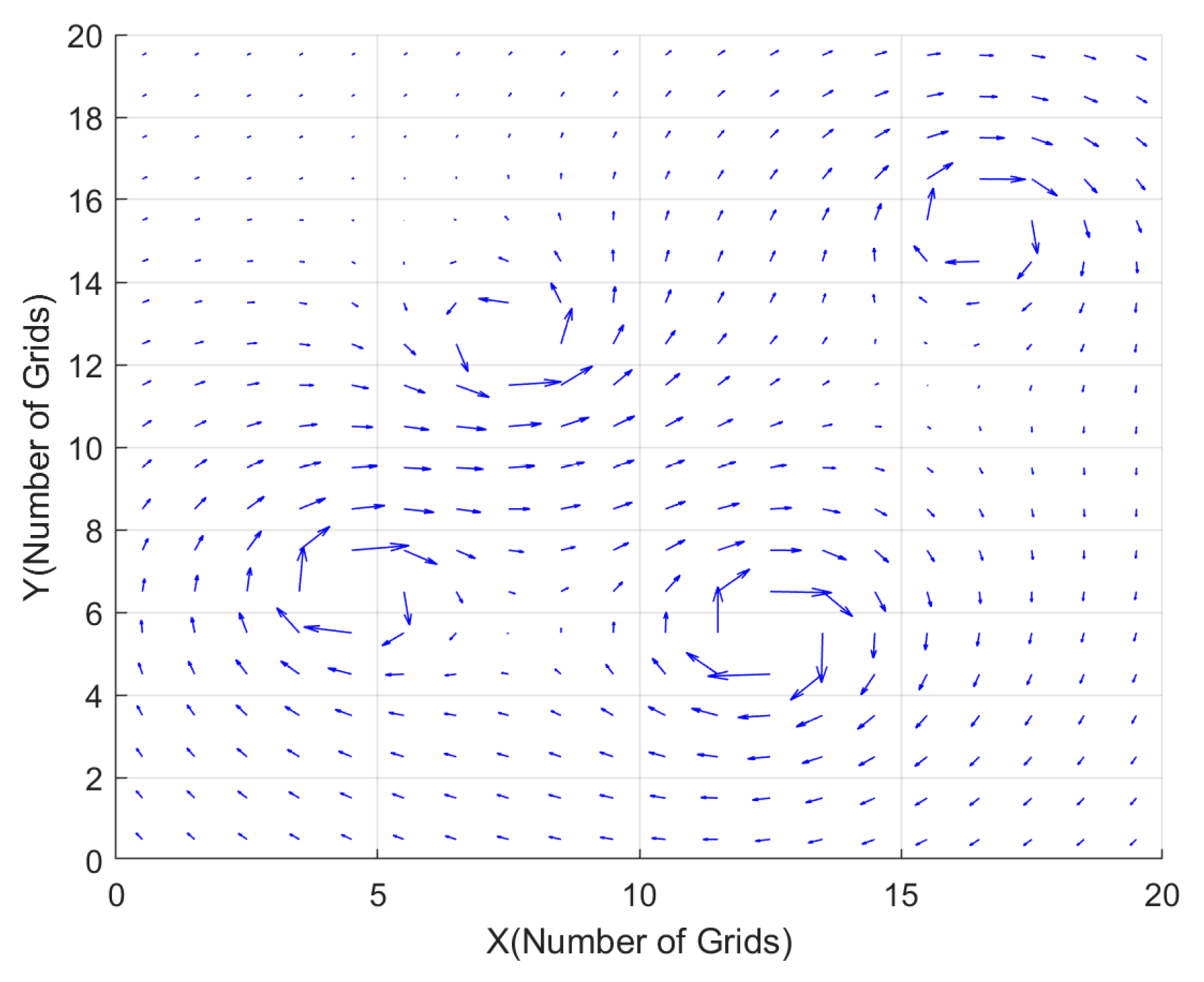
Here, $(x,y)$ are the coordinates of the current point in the flow field, $R$ is the distance from this point to the vortex center, $p_x$ is the $\mathrm{x}$-coordinate of the vortex center $p$, $p_y$ is the $y$-coordinate of the vortex center $p$, $U$ is the velocity component of the ocean current in the $x$-direction, $V$ is the velocity component in the $y$-direction, and $q$ is the intensity of the vortex. The ocean current environment where multiple eddies converge is shown in Figure 1.

2.2. Ant Colony Optimization Model

The ACO algorithm mimics the ant foraging behavior for path planning [21]. As ants traverse paths, they deposit pheromones. The concentration of these pheromone trails guides the route selection of subsequent ants. In the initial exploration phase, paths are chosen randomly [22]. Through a positive feedback mechanism, shorter paths accumulate higher pheromone concentrations more rapidly, thereby attracting more ants. This process eventually leads the entire colony to converge on the shortest path, thus achieving optimal path planning [23].

In the ACO algorithm, ants determine their next node selection based on the pheromone concentrations along the paths [24]. The transition probability $P_{ij}$ for ant $k$ to move from node $i$ to node $j$ at time $t$ is defined by Equation (2), where ${\eta }_{ij}$ denotes the heuristic function given in Equation (3).

$$P_{ij}=\left\{\begin{array}{r}{\displaystyle \frac{{\tau }_{ij}^{\alpha }(t){\eta }_{ij}^{\beta }(t)}{{\displaystyle \sum _{S\in (allowed(k))}{\tau }_{ij}^{\alpha }(t){\eta }_{ij}^{\beta }(t)}}},S\in (allowed(k))\\ 0,S\notin (allowed(k))\end{array}\right.$$

(2)

$${\eta }_{ij}={\displaystyle \frac{1}{d_{ij}}}$$

(3)

$$d_{ij}=\sqrt{{(x_i-x_j)}^2+{(y_i-y_j)}^2}$$

(4)

In the aforementioned formula, $\alpha$ denotes the pheromone weighting coefficient; $\beta$ represents the heuristic function weighting coefficient; ${\tau }_{ij}(t)$ refers to the pheromone concentration function; $allowed(k)$ indicates the set of feasible nodes; ${\eta }_{ij}^{\beta }(t)$ corresponds to the distance heuristic function; $(x_i,y_i)$ and $(x_j,y_j)$ specify the coordinate positions of node $i$ and node $j$, respectively; and $d_{ij}$ defines the Euclidean distance between node $i$ and node $j$.

Once all ants have completed a path search, the pheromone concentration on each path is updated under the influence of the evaporation coefficient $\rho (0<\rho <1)$. The pheromone update formula is given below.

$${\tau }_{ij}(t+1)=(1-\rho ){\tau }_{ij}(t)+\Delta {\tau }_{ij}(t)$$

(5)

$$\Delta {\tau }_{ij}(t)={\displaystyle \sum _{k=1}^m\Delta {\tau }_{ij}^k(t)}$$

(6)

$$\Delta {\tau }_{ij}(t)=\left\{\begin{array}{l}{\displaystyle \frac{Q}{L_k}},(An{t}_k\in Path(i,j) )\\ 0,(An{t}_k\notin Path(i,j) )\end{array}\right.$$

(7)

In the above equation, $Q$ denotes the total amount of pheromone carried by the ants; $L_k$ represents the total path length traversed by ant $k$; $m$ is the total number of ants in each iteration; $\Delta {\tau }_{ij}^k(t)$ indicates the amount of pheromone released by ant $k$ on $Path(i,j)$; $\Delta {\tau }_{ij}(t)$ signifies the total pheromone deposited by all ants on $Path(i,j)$ [25].

The conventional ACO algorithm primarily optimizes path length, as defined in Equation (3), which fails to adequately capture complex dynamic environmental factors. Moreover, the algorithm depends on a cost function and a pheromone update strategy that use Euclidean distance as the sole heuristic metric, as formulated in Equation (7). Although this framework guarantees basic goal reachability, it fails to address the multifaceted requirements of complex marine environments, which include energy consumption, motion smoothness, and operational endurance [26].

3. IMOACO Algorithm

3.1. Constructing the Objective Function and State Transition Function

3.1.1. Constructing the Objective Function

To address the operational requirements of rescue AUVs for short path length, low energy consumption, and smooth trajectories, a comprehensive multi-criteria path cost evaluation function is developed. This function integrates path length, energy consumption, and smoothness, enabling the path planning algorithm to dynamically adapt to complex environments. Furthermore, a novel state transition rule, optimized based on heading angle, is designed. This rule quantifies the angular relationship between the ocean current vector and the AUV’s navigation direction, establishing a state transition matrix that incorporates ocean current direction information. This enhancement significantly improves the algorithm’s adaptability to dynamic ocean current environments. Additionally, a multi-criteria influenced pheromone update mechanism is introduced. This mechanism ensures that the path selection process during pheromone iteration is directly guided by the comprehensive evaluation metrics derived from the cost function.

Objective Function 1: Shortest Path

To quantify the path length, this paper employs the Euclidean distance as the metric for calculating the length of each path segment. The path length metric is presented as follows:

$$P=\left\{p_1,p_2,p_3,p_4,\dots \dots ,p_n\right\}$$

(8)

$$L(p_i,p_{i+1})=\sqrt{{(x_{i+1}-x_i)}^2+{(y_{i+1}-y_i)}^2}$$

(9)

$$L(p)={\displaystyle {\sum }_{i=1}^{n}L(p_i,p_{i+1})}$$

(10)

where $P$ denotes the set of paths, $p_i$ represents the i-th node on the path, $p_{i+1}$ denotes the $i+1$-th node on the path, $L(p_i,p_{i+1})$ signifies the Euclidean distance between nodes $i$ and $i+1$ on path $p$, and $L(p)$ denotes the total length of path $p$.

Objective Function 2: Path Energy Consumption

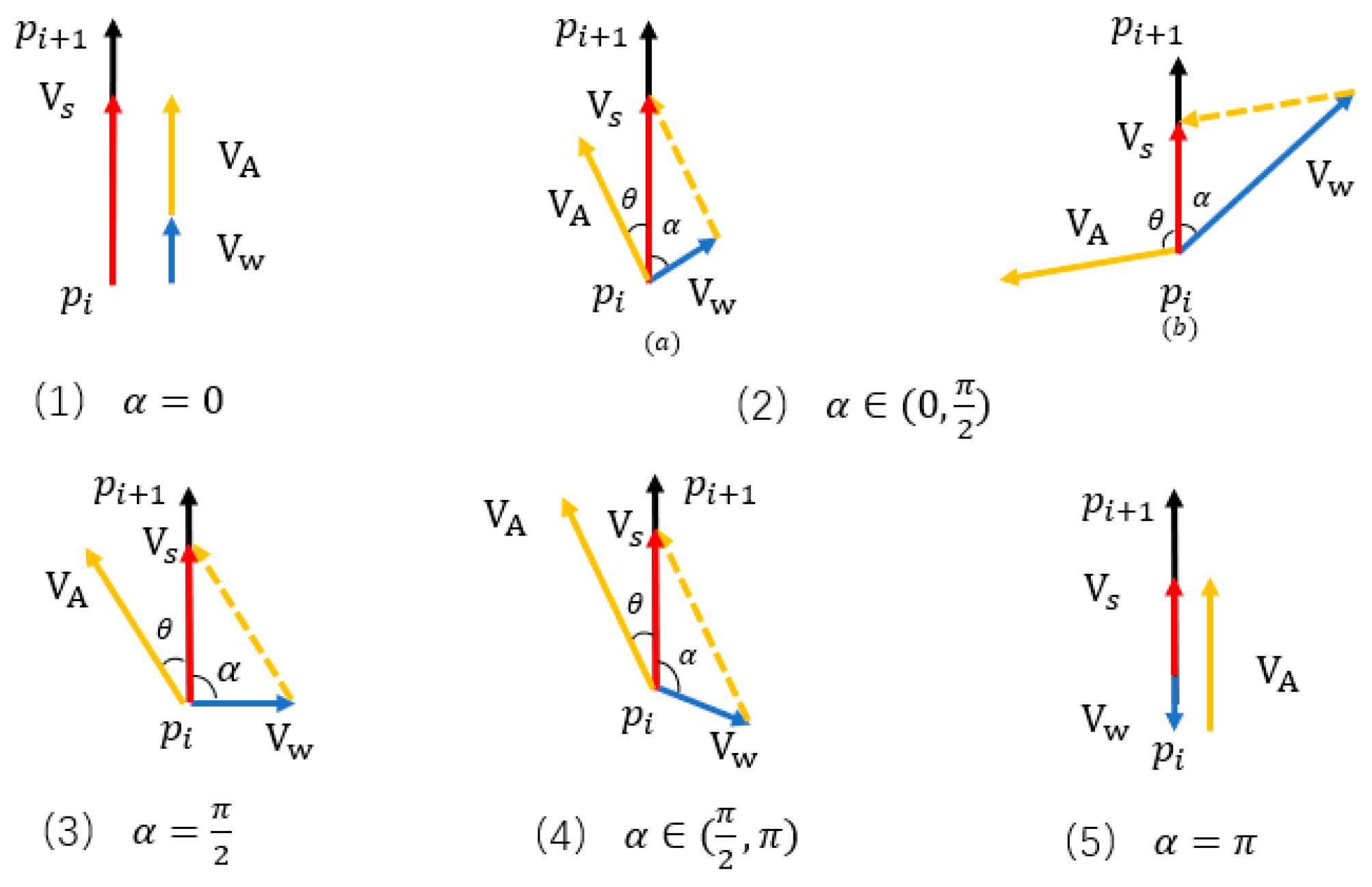
In ocean current environments, AUVs exhibit low inertia and are highly susceptible to hydrodynamic disturbances. Navigating against currents substantially increases propulsion energy expenditure and induces significant heading deviations. A path planning algorithm incorporating ocean current distribution features can dynamically optimize the AUV’s trajectory by steering it toward favorable currents or away from intense adverse flow regions, thus effectively minimizing overall energy consumption, as depicted in Figure 2.

Here, $p_i$ represents the current AUV position, $p_{i+1}$ denotes the next path node; $V_w$ indicates the current ocean current velocity; $V_A$ signifies the AUV’s propulsion speed in still water; $V_s$ represents the AUV’s combined velocity; $\alpha$ is the angle between the actual travel direction and the current ocean current; $\theta$ is the angle between the AUV’s heading and its actual travel direction. By aligning the AUV’s motion with favorable currents, this strategy minimizes propulsion resistance, thereby guaranteeing minimal energy expenditure for the current path segment.

$${\mathsf{V}}_{\mathsf{s}}={\mathsf{V}}_{\mathsf{A}}\cos \theta +{\mathsf{V}}_{\mathsf{w}}\cos \alpha$$

(11)

The energy dissipation formula for AUVs in ocean current environments [27], as shown in (12):

$$E=q{V}_A^3{\displaystyle \frac{\left|L_{p_i{p}_{i+1}}\right|}{V_s}}$$

(12)

In this equation, $q$ is the AUV drag coefficient, $V_A$ is the AUV propulsion speed in still water, $L_{p_i{p}_{i+1}}$ is the distance from path point $p_i$ to $p_{i+1}$, $V_{\mathrm{s}}$ is the AUV combined speed, and $E$ is the energy consumption of the AUV along this path.

Objective Function 3: Path Smoothness

Path smoothness reflects the continuity and stability of an AUV’s trajectory, which is critically influenced by the variation of turning angles along the path. Implementing smoothness strategies can effectively suppress redundant steering maneuvers, reduce attitude fluctuations, minimize sensor-derived errors, and consequently enhance mission accuracy and operational reliability. The formula for calculating the path turning angle is defined as follows:

$$\theta =\mathrm{acos}{\displaystyle \frac{p_{j-1}{p}_j•p_j{p}_{j+1}}{\left|\left|p_{j-1}{p}_j\right|\right|•\left|p_j{p}_{j+1}\right|}},2\le j\le n$$

(13)

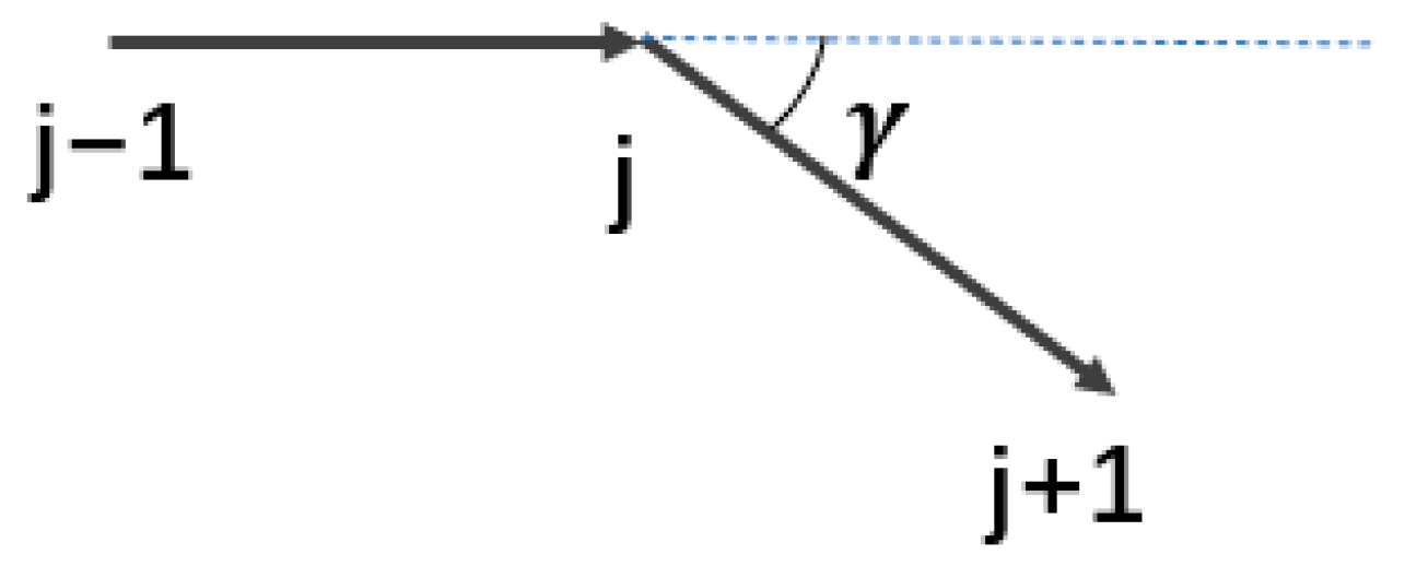
As shown in Figure 3, points $j-1$, $j$, and $j+1$ are three adjacent target points; $p_{j-1}{p}_j$ is the vector from point $p_{j-1}$ to $p_j$; $p_j{p}_{j+1}$ is the vector from point $p_j$ to $p_{j+1}$; $\left|p_{j-1}{p}_j\right|$ is the magnitude of vector $p_{j-1}{p}_j$; $\left|p_j{p}_{j+1}\right|$ is the magnitude of vector $p_j{p}_{j+1}$; $\gamma$ is the angle between the two vectors; $n$ is the number of path nodes.

Min-max normalization is applied to the metrics of path length, energy consumption, and turning angle, with the calculation formula presented below.

$$x_{ij}^{\prime }={\displaystyle \frac{x_{ij}-\min (x)}{\max (x)-\min (x)}}$$

(14)

$x$ denotes the raw dataset of a specific evaluation metric (such as path length, energy consumption, or number of turns) across all candidate paths; $x_{ij}$ represents the raw numerical value of the $j$-th evaluation metric for the $i$-th path; $x_{ij}^{\prime }$ denotes the corresponding normalized dimensionless value, ranging between [0, 1]. $\max (x)$ and $\min (x)$ respectively denote the maximum and minimum values of this metric across all paths.

3.1.2. Ocean Current Direction State Transfer Function

When there is an angle between the AUV’s heading and the ocean current vector, additional propulsion must be applied to counteract the lateral shear force induced by the current. This leads to reduced propulsion efficiency, increased trajectory deviation, and speed attenuation. Conversely, a positively coupled alignment between the heading and the current direction can lower energy consumption, enhance trajectory stability, and extend operational endurance [28]. To address this, the IMOACO algorithm introduces a heuristic function based on the heading–current angle. This function quantifies the spatial relationship between the two vectors to dynamically optimize heading selection. Under kinematic constraints, it guides the AUV toward downstream movement, thereby achieving minimized energy consumption. The expression of the heuristic function is as follows:

$$Angl{e}_{ij}={\displaystyle \frac{1}{e^{\delta }}}$$

(15)

In the above formula, $e$ is the natural constant; $\delta$ is the angle between the AUV heading and the ocean current direction, measured in radians. The heuristic information function $Angl{e}_{ij}$ is inversely proportional to $\delta$: the smaller the $\delta$ value is, the larger the $Angl{e}_{ij}$ value becomes, indicating that the path is less affected by ocean currents and thus has a higher probability of being selected.

Based on the heading–current angle heuristic function, a state transition function is constructed. The improved transition probability $p_{ij}^k(t)$ is calculated as follows:

$$p_{ij}^k(t)=\left\{\begin{array}{c}{\displaystyle \frac{[{\tau }_{ij}{(t)}^{\alpha }]\ast [{\eta }_{ij}{(t)}^{\beta }][Angl{e}_{ij}{(t)}^{\gamma }]}{{\displaystyle \sum s\in J_k(i)}[{\tau }_{ij}{(t)}^{\alpha }]\ast [{\eta }_{ij}{(t)}^{\beta }][Angl{e}_{ij}{(t)}^{\gamma }]}},if j\in J_k(i)\\ 0, else\end{array}\right.$$

(16)

In this equation, ${\tau }_{ij}(t)$, ${\eta }_{ij}(t)$, and $Angl{e}_{ij}(t)$ represent the pheromone concentration, expected heuristic function, and heading-to-current angle heuristic function between node $i$ and node $i+1$ at time $t$, respectively; $\alpha$ denotes the pheromone heuristic factor; $\beta$ denotes the expected heuristic factor; $\gamma$ denotes the heading-to-current angle heuristic factor.

3.2. Improving the Heuristic Function

The IMOACO algorithm reconstructs the heuristic function. This is achieved through the establishment of a comprehensive evaluation system that incorporates multiple constraints, including path length, energy consumption, and turning angle. The improved heuristic function ${\eta }_{ij}$ is expressed as in Equation (17).

$${\eta }_{ij}={\displaystyle \frac{1}{w_1{L}_{ij}+w_2{E}_{ij}+w_3{\theta }_{ij}}}$$

(17)

Here, $L_{ij}$ denotes the path length of this segment, $E_{ij}$ represents the energy consumption of the path, ${\theta }_{ij}$ indicates the path turning angle, and $w_1$, $w_2$, $w_3$ are the respective weights assigned to path length, energy consumption, and path turning angle.

3.3. Improving Pheromone Refresh Strategies

The IMOACO algorithm extends the conventional path-distance weighting scheme by integrating energy consumption and smoothness factors. Furthermore, by introducing adaptive weighting factors into the pheromone update rule, the algorithm dynamically balances these metrics, favoring energy-efficient and smooth paths.

$$\Delta {\tau }_{ij}^k={\displaystyle \frac{Q}{COST}}$$

(18)

$$COST=w_{1}L+w_{2}E+w_3\theta$$

(19)

To enable the algorithm to balance multiple path possibilities and prevent premature convergence of the ACO, a dynamic evaporation factor is introduced.

$$\rho (NC)={\rho }_{\max }-({\rho }_{\max }-{\rho }_{\min })•{\displaystyle \frac{NC}{N{C}_{\max }}}$$

(20)

In the above formulation, $\rho (NC)$ represents the pheromone evaporation factor at iteration $NC$; ${\rho }_{\max }$ denotes the maximum evaporation factor; ${\rho }_{\min }$ is the minimum evaporation factor; and $N{C}_{\max }$ specifies the maximum number of iterations. The complete pheromone update formula is given as follows:

$${\tau }_{ij}(t+1)=(1-\rho )•{\tau }_{ij}(t)+{\displaystyle {\sum }_{k=1}^m\Delta {\tau }_{ij}^k}(t)$$

(21)

3.4. Adaptive Adjustment of Heuristic Function Weights

In multi-objective path planning, traditional subjective weighting methods, which rely on expert experience to construct judgment matrices, exhibit limitations in dynamic marine environments [28,29]. Small-scale TSP instances can be solved exactly via integer linear programming or branch-and-bound methods; the dynamic nature of ocean current disturbances and the large-scale search spaces in AUV missions create computational feasibility barriers for exact methods in real-time applications. Furthermore, this study prioritizes practical engineering objectives in rescue scenarios, such as mission efficiency, energy economy, and trajectory stability, rather than focusing exclusively on theoretical TSP solutions. To address the co-optimization requirements for path length, energy consumption, and smoothness in the Traveling Salesman Problem (TSP)—which serves as a simplified model for multi-target sequencing in AUV path planning—a data-driven dynamic entropy weight method is proposed and compared with meta-heuristic methods to ensure its applicability in complex marine environments.

Step 1: Initial Weight-Guided Search: Initial weight combinations are set based on prior experimental data to drive the ant colony algorithm toward generating superior paths.

Step 2: Data Normalization: A matrix composed of $c$ candidate paths and $v$ evaluation metrics is constructed and undergoes normalization to eliminate dimensional differences. The normalization formula is as follows:

$$x_{hq}^{\prime }={\displaystyle \frac{\max \{l_{1q},l_{2q},\cdots ,l_{cq}\}-l_{hq}}{\max \{l_{1q},l_{2q},\cdots ,l_{cq}\}-\min \{l_{1q},l_{2q},\cdots ,l_{cq}\}}}$$

(22)

In the above formula, $l_{hq}$ denotes the value of the $q$-th evaluation metric for the $q$-th path; $l_{hq}^{\prime }$ represents the standardized value of this metric; and $l_{1q},l_{2q},l_{3q},\cdots ,l_{cq}$ form the set of values of the $q$-th evaluation metric corresponding to the 1st, 2nd, …, up to the $c$-th path.

Step 3: Calculate the proportion $p_{hq}$ of the $h$-th path under the $q$-th evaluation indicator relative to that indicator.

$$p_{hq}={\displaystyle \frac{l_{hq}^{\prime }}{{\displaystyle {\sum }_{h=1}^c{l}_{hq}^{\prime }}}}h=1,2,\dots c q=1,2,\dots v$$

(23)

Step 4: Calculate the entropy value $a_q$ of the $q$-th evaluation item indicator.

$$a_q=-{\displaystyle \frac{1}{\ln c}}{\displaystyle {\sum }_{h=1}^c{p}_{hq}\ln p_{hq}} q=1,2,\dots v$$

(24)

Step 5: Calculate the information entropy redundancy $d_q$ of the $q$-th evaluation indicator.

$$d_q=1-a_q$$

(25)

Step 6: Calculate the weight $w_q$ of the $q$-th evaluation indicator.

$$w_q={\displaystyle \frac{d_q}{{\displaystyle {\sum }_{q=1}^c{d}_q}}}$$

(26)

Step 7: Establish an entropy weight–ant colony cooperative optimization framework. Integrate the multi-objective weighting parameters generated by the dynamic entropy weight method into the cost function of the improved ant colony algorithm to construct a multi-criteria cost model that incorporates path length, energy consumption, and smoothness. By employing a collaborative update mechanism that combines heuristic probability and pheromone gradient, adaptive optimization of the path search is achieved, guiding the population to converge toward the global optimal solution region. It should be noted that the evaluation matrix consists of paths generated by all ants in the current iteration, with each row corresponding to the normalized metric value of a path. Entropy weights are updated immediately after each iteration concludes.

Step 8: Closed-loop iteration and autonomous convergence: Check whether the convergence conditions are met. Satisfaction of the convergence condition means that the change in the cost function in Equation (8) is less than a certain threshold. If satisfied, proceed to Step 9; otherwise, return to Step 7.

Step 9: Output the optimal path.

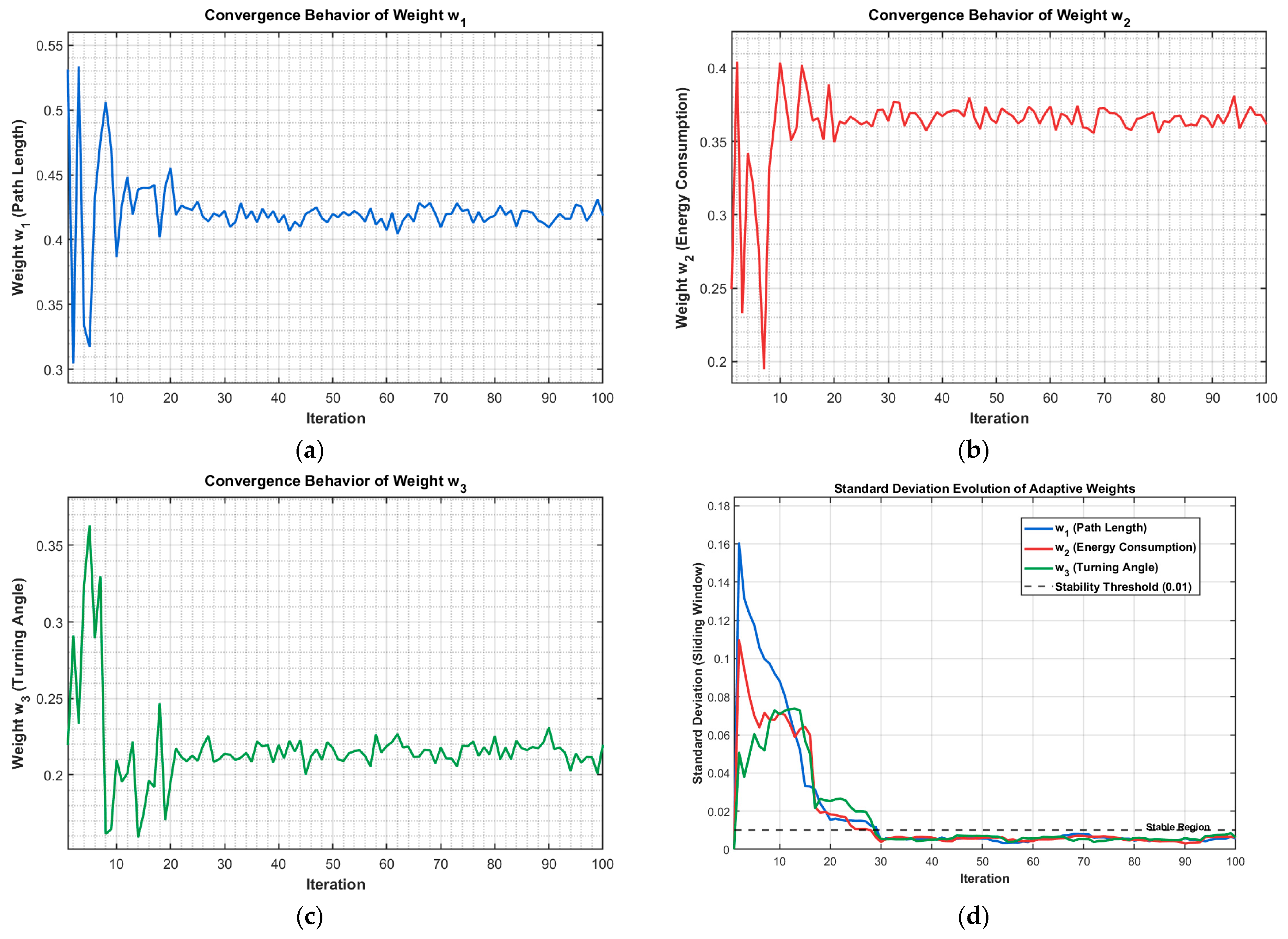
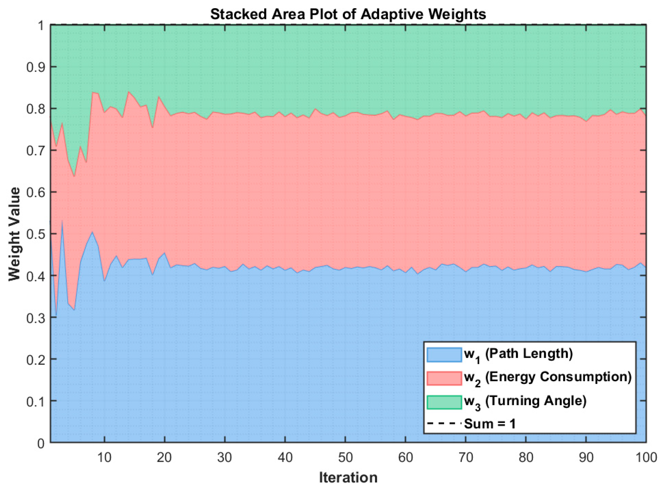
Figure 4 and Figure 5 illustrate the convergence behavior of adaptive weights during the iteration process in a specific multi-objective task scenario. The three weights exhibit intense oscillations during the initial iteration phase, followed by rapid convergence. They eventually stabilize in the later iteration stages, with their respective means converging to approximately 0.418, 0.367, and 0.215. The standard deviation of all three weights decreases as iterations progress, consistently remaining below 0.01 in the later stages.

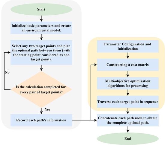
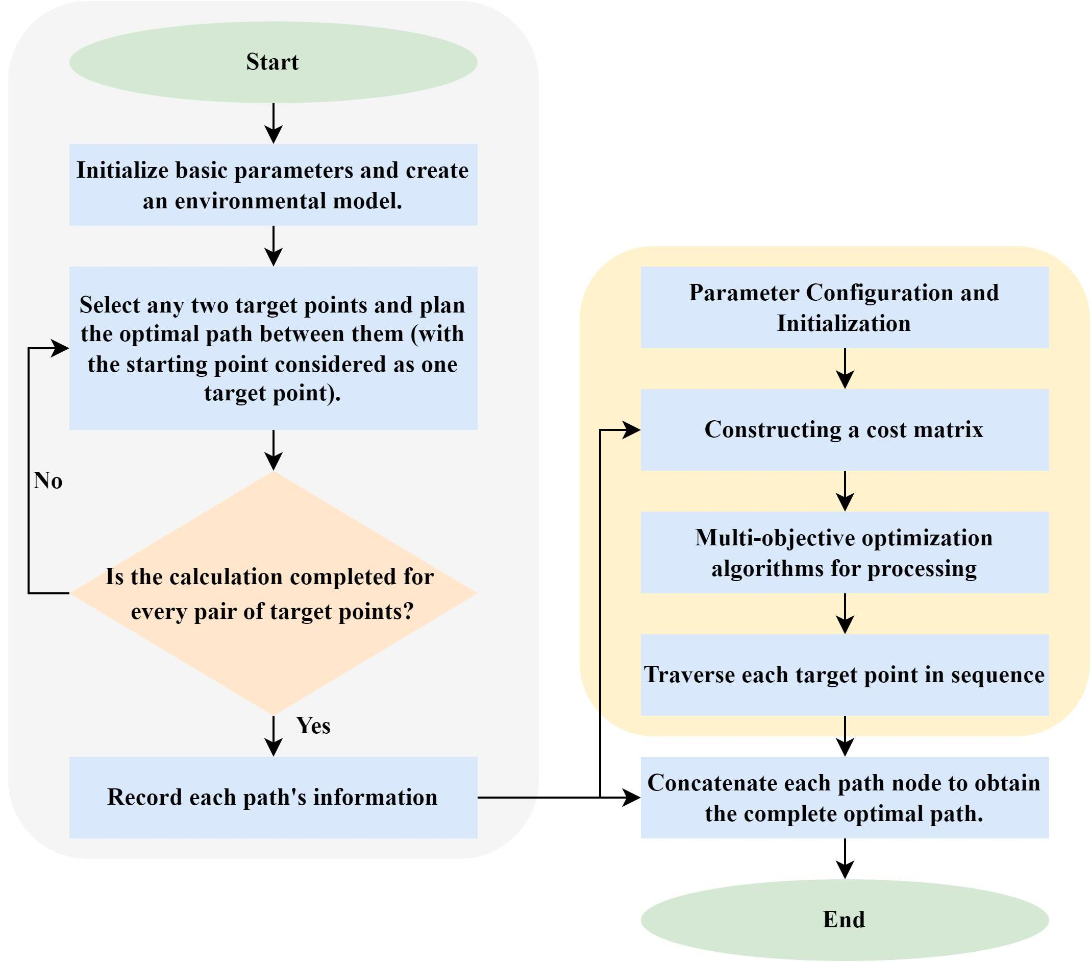
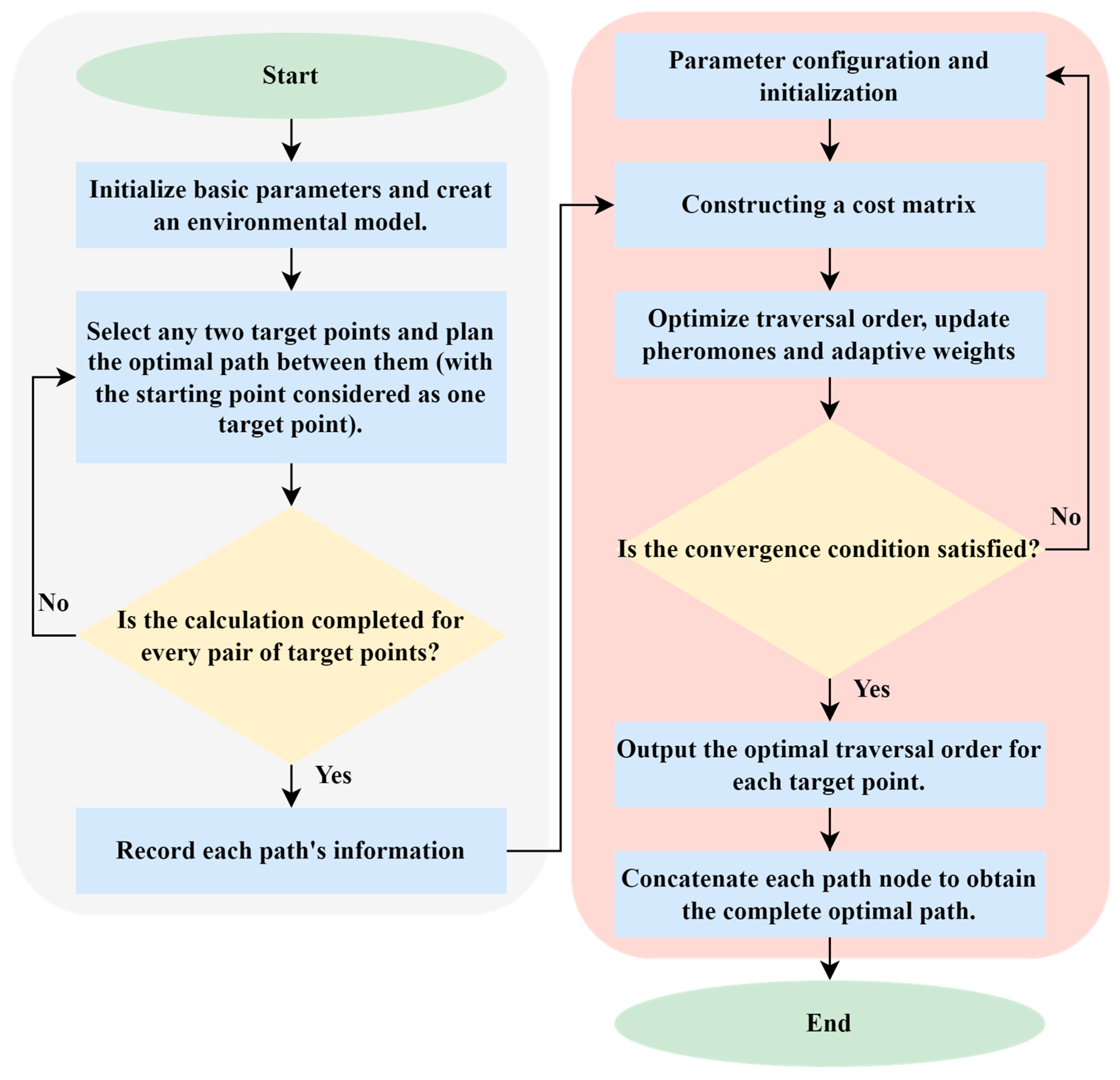
The IMOACO algorithm flow is shown in Figure 6. The pseudocode for IMOACO is shown in Algorithm 1.

The IMOACO algorithm enhances the heuristic function of the conventional ACO by incorporating a multi-criteria cost evaluation function. It employs a data-driven dynamic entropy weight method to assess function weights and introduces an adaptive adjustment strategy for the pheromone evaporation rate, thereby improving the algorithm’s convergence speed and stability.

Algorithm 1 IMOACO
Input: Map matrix G, start point s, target set T, ocean current field
Output: Optimal path sequence Route_best
1:	Initialize pheromone matrix and heuristic information
2:	for each target point pair (i,j) do
3:	while NC ≤ NC_max do
4:	for each ant k = 1 to m do
5:	Construct path and calculate cost using ACO
6:	end for
7:	Update pheromone concentration, NC ← NC + 1
8:	end while
9:	Store optimal path and cost for pair (i,j)
10:	end for
11:	while iter ≤ iter_max do
12:	for each ant k = 1 to m do
13:	Construct target visiting sequence and calculate cost
14:	end for
15:	Adaptively update weights, update global best and pheromone
16:	iter ← iter + 1
17:	end while
18:	return Route_best

4. Simulation Verification

To verify the feasibility and effectiveness of the proposed IMOACO algorithm in addressing path planning challenges for rescue AUVs, diverse simulation environments were constructed to comprehensively evaluate its performance.

4.1. Single-Objective Two-Dimensional Environment: Simulation Verification of Effectiveness and Advancement

The single-objective simulation parameter settings are shown in

Table 2. Parameter combinations.

Parameter	Value
Pheromone-Inspired Factor	2
Expectation-Inspiration Factor	10
Ocean Current Angle Factor	0.5
Pheromone volatilization factor	0.3
Number of ants	50
Maximum number of iterations	100
Maximum pheromone capacity	1
$w_1$	0.4
$w_2$	0.4
$w_3$	0.2

.

4.1.1. Single-Objective Environment Effectiveness Simulation Verification

To evaluate the effectiveness of the single-objective approach and reduce the randomness of experimental results, simulations were performed on a 20 × 20 grid map (equivalent to 600 m × 600 m) with obstacles. Four different start-end point configurations were selected, and 20 trials were conducted for each configuration, with the average values used for comparison.

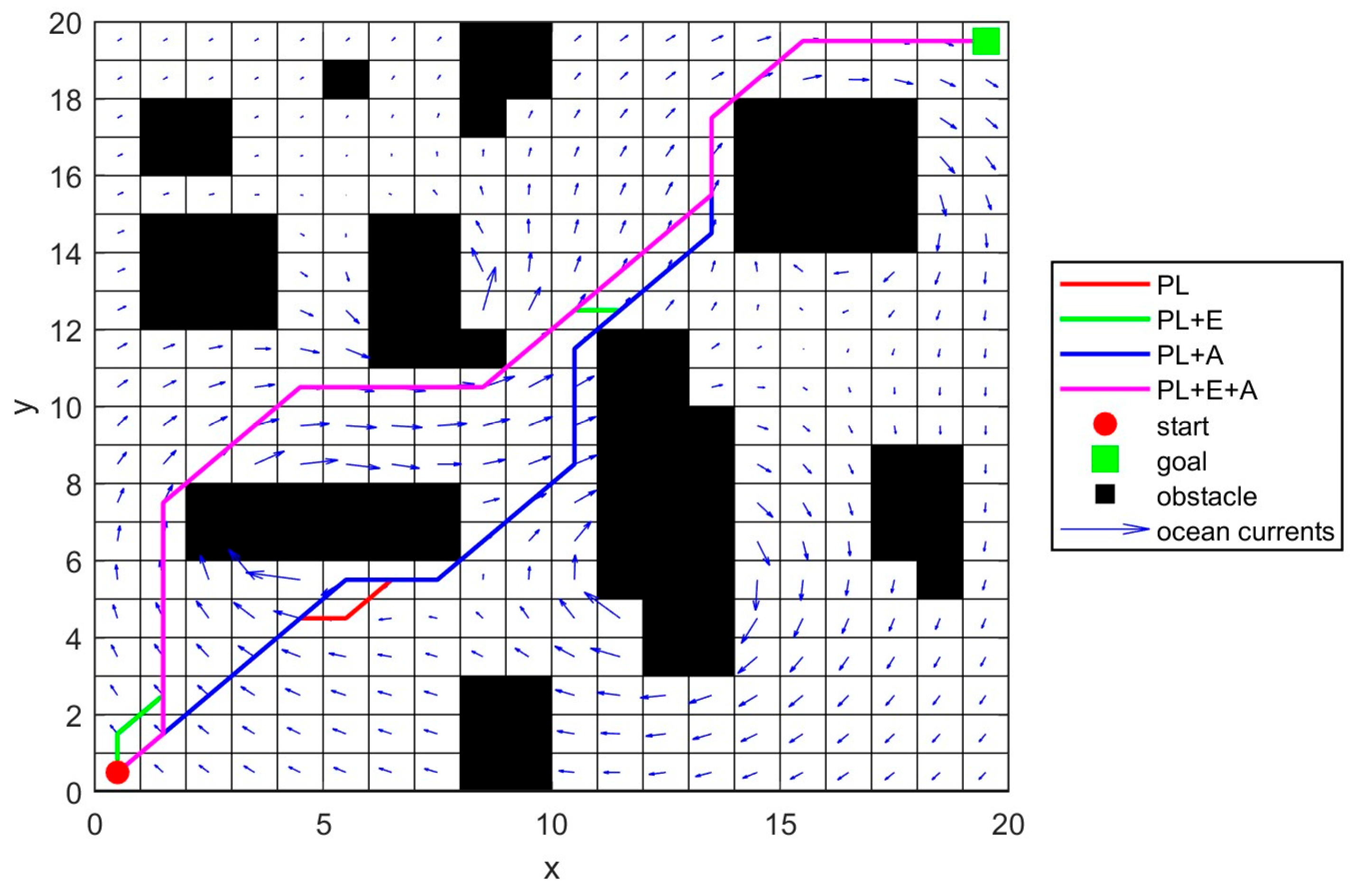
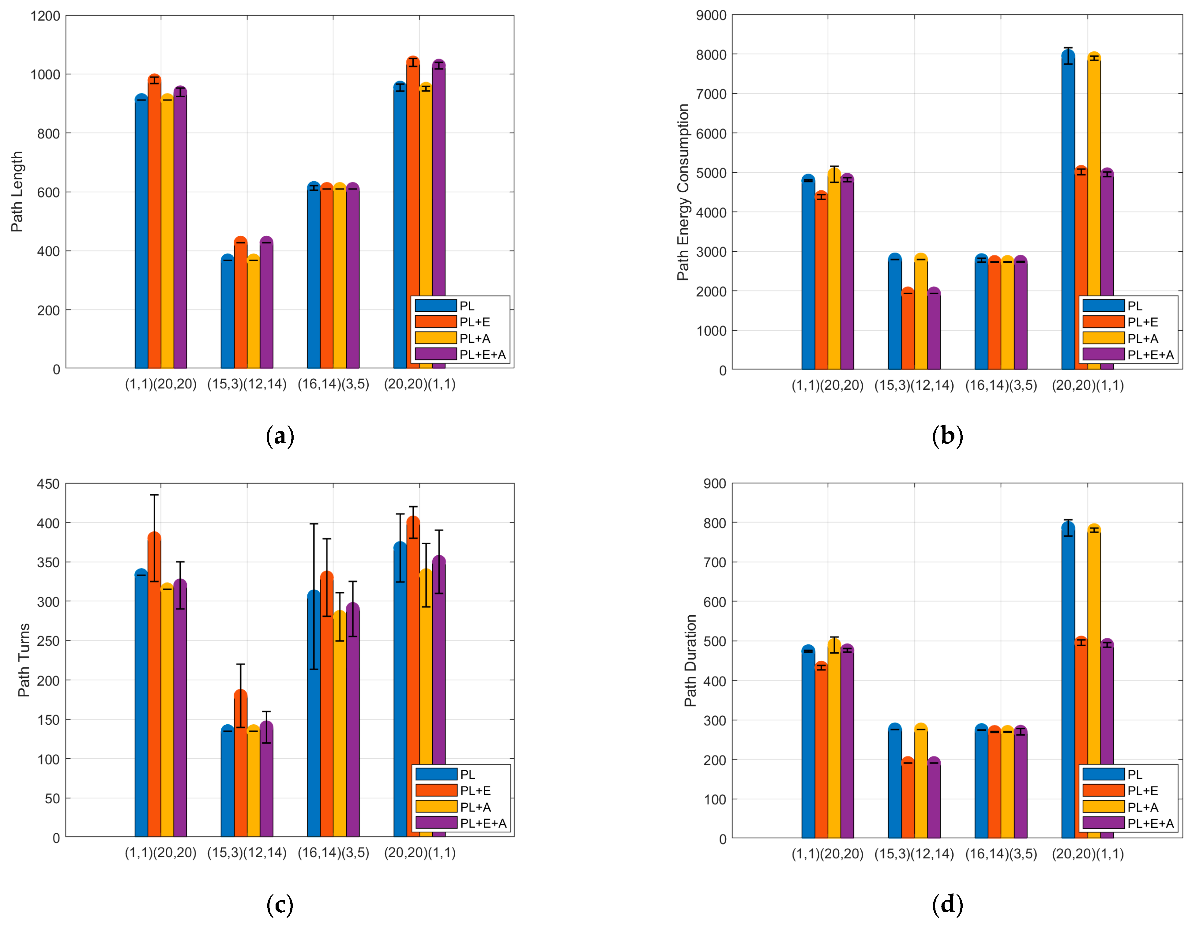
The simulation results are presented in Figure 7. In the figure, the red path represents the strategy considering only the path length (PL), green corresponds to path length and energy consumption (PL + E), blue indicates path length and turning angle (PL + A), and purple denotes the integration of path length, energy consumption, and turning angle (PL + E + A). The statistical results of the experiments are shown in Figure 8.

Simulation results indicate that the proposed IMOACO algorithm (PL + E + A) surpasses all comparative algorithms in path planning performance. Specifically, it reduces the path length by 5.2%, decreases energy consumption by 21.3%, and cuts the turning angle by 50% relative to the PL + E, PL, and PL + E benchmarks, respectively. In terms of mission duration, PL + E + A achieves a 21.4% reduction compared to PL. The proposed algorithm achieves optimal overall performance across multiple metrics, including path length, energy efficiency, and smoothness, thereby validating the comprehensive advantages of multi-objective optimization in enhancing path economy, energy efficiency, and smoothness.

4.1.2. Single-Objective Environment Robustness and Advanced Simulation Verification

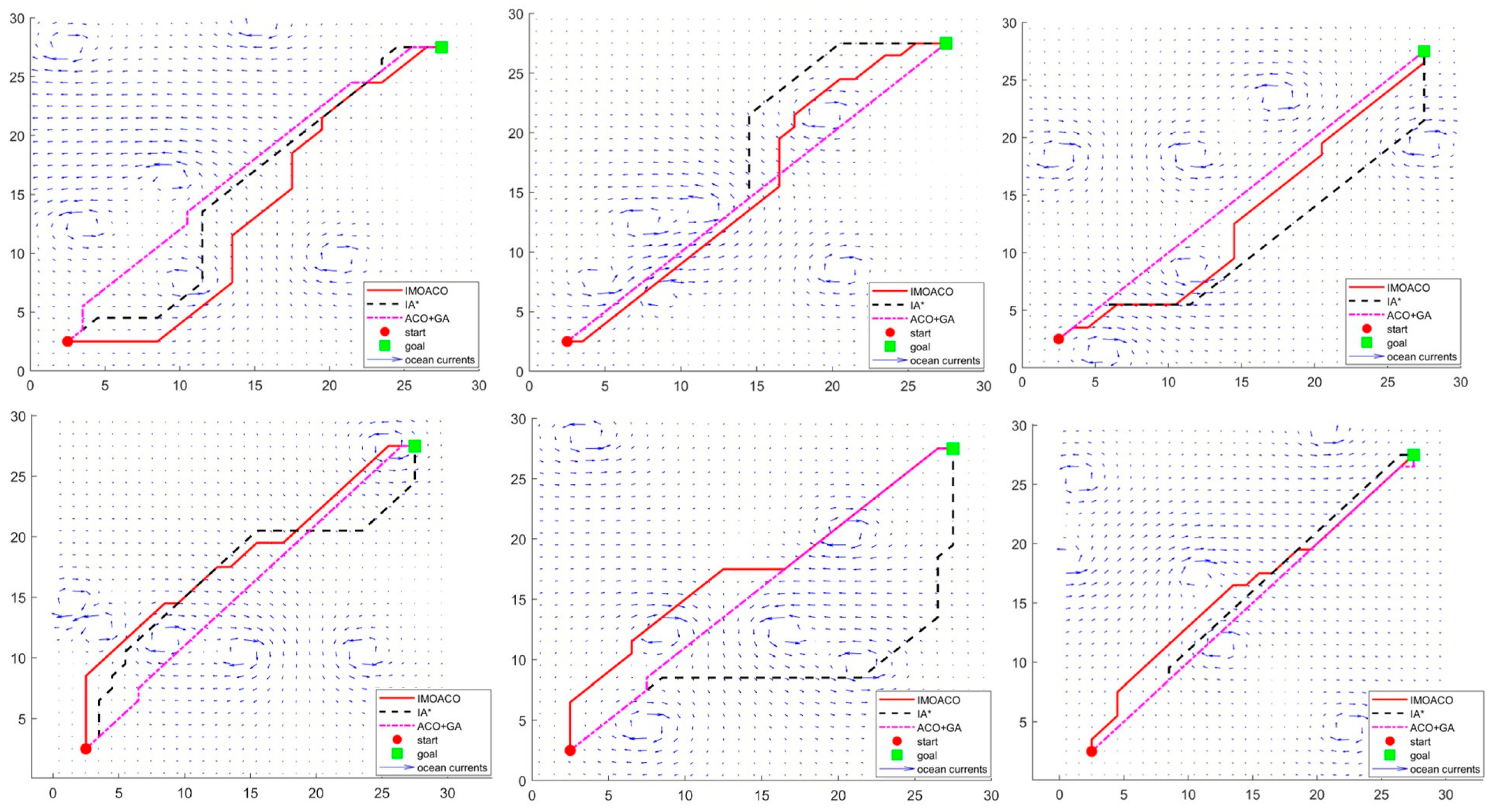
To verify the robustness and advancement of the proposed algorithm, the IMOACO algorithm was compared with the IA* algorithm [30] and the ACO + GA algorithm [31]. The three algorithms were tested in six randomly generated scenarios, each containing six vortices. The simulation environment was set as a 30 × 30 grid corresponding to a 900 m × 900 m task area. The results of six randomized simulation runs are illustrated in Figure 9, and the path evaluation metrics for each algorithm are summarized in

Table 3. Cost metrics for three algorithms across six scenarios.

Algorithm	Scenario 1	Scenario 2	Scenario 3	Scenario 4	Scenario 5	Scenario 6
IMOACO	13.944	11.481	11.226	12.796	12.672	11.581
IA*	14.004	11.626	12.216	13.648	14.621	11.656
ACO + GA	14.515	12.824	13.146	14.019	13.396	13.163

. The data in the table represent the normalized cost metrics for each algorithm under various scenarios.

Based on the simulation results from six randomized ocean current scenarios, the IMOACO algorithm achieved optimal solutions in all cases. The average path cost of IMOACO (12.403) was reduced by 4.36% compared to the IA* algorithm (12.969) and by 8.86% compared to the hybrid genetic–ant colony algorithm (ACO + GA, 13.608). These results effectively demonstrate the advanced performance and robustness of the IMOACO algorithm under stochastic conditions.

4.2. Multi-Objective Two-Dimensional Environment Effectiveness and Advanced Simulation Verification

4.2.1. Adaptive Weight Effectiveness Validation

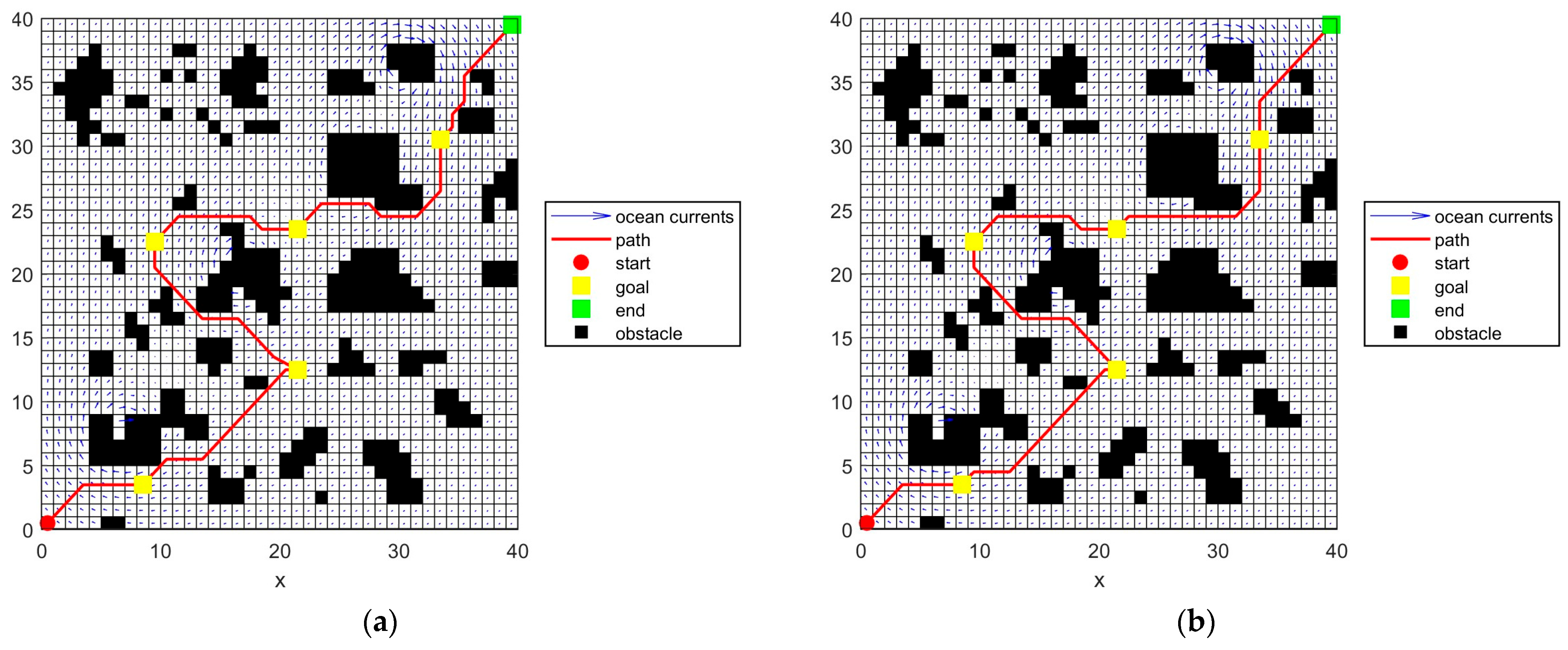
To verify the effectiveness of the adaptive weighting strategy, a 40 × 40 grid map was established, representing a task area of 1200 m × 1200 m. The resulting paths are presented in Figure 10, and the corresponding metrics for each path are provided in

Table 4. Comparison of various metrics for two algorithms: Fixed Weight and Adaptive Weight.

Algorithm	Cost	Length (m)	Energy Consumption (J)	Turning Angle (°)	Duration (s)
Fixed Weight	34.04	2582.49	15,802.62	990	1562.06
Adaptive Weight	33.75	2557.64	15,638.79	990	1545.87

.

Figure 10 compares simulation results of the IMOACO algorithm’s path planning in complex environments. Figure 10a shows the path generated using a fixed-weight strategy, while Figure 10b presents the path produced by the adaptive weight strategy based on the entropy weight method. Compared to the fixed-weight approach, the adaptive weighting algorithm yields a more balanced spatial path distribution. By dynamically adjusting weight parameters in the multi-objective evaluation function, the algorithm effectively mitigates path overlap in local regions and avoids suboptimal path selection.

As quantified in Table 4, the adaptive weighting strategy achieves the following improvements: the comprehensive cost decreases from 34.043 to 33.747 (a 0.87% reduction), the path length shortens from 2582.49 m to 2557.64 m (a 0.97% decrease), and the total energy consumption drops by 163.83 J (a 1.04% reduction). These results demonstrate that the dynamic weight allocation mechanism based on the entropy weight method significantly enhances both the objectivity of evaluation weights and the overall path planning performance.

4.2.2. Simulation Verification of Advanced Features

This section presents the simulation results comparing the path planning performance of the proposed IMOACO algorithm with conventional ACO and IA* algorithms. The parameters used in IMOACO are summarized in

Table 5. Parameters of the multi-objective traversal optimization algorithm.

Parameter	Value
Pheromone-Inspired Factor	2
Expectation-Inspiration Factor	6
Maximum Pheromone Evaporation Factor	0.8
Minimum Pheromone Evaporation Factor	0.4
Number of ants	20
Maximum number of iterations	100

, followed by a comparative analysis of the experimental results.

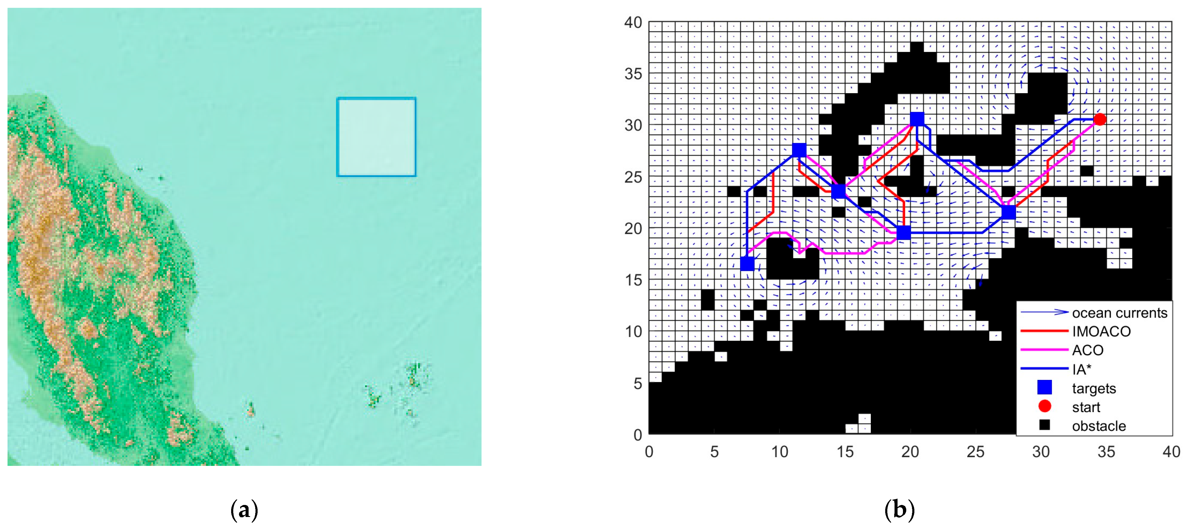
To simulate a search and rescue scenario, a geographical area within longitude E 105.3–106.2° and latitude N 5.8–6.8° was discretized into a 40 × 40 grid map, with each grid cell representing a 100 m × 100 m area. The total mission area thus covers 4000 m × 4000 m. Simulations of the three algorithms were performed in this environment. The resulting paths are illustrated in Figure 11, and the corresponding evaluation metrics are provided in

Table 6. Comparison of various metrics for three algorithms in the first simulation.

Algorithm	Length (m)	Energy Consumption (J)	Turning Angle (°)	Duration (s)
IA*	6737.51	33,431.19	990	3304.61
ACO	6484.07	37,630.27	1710	3719.68
IMOACO	6503.14	32,094.89	945	3172.51

.

The comparative results in Table 6 demonstrate that the IMOACO algorithm achieves significant comprehensive advantages in large-scale multi-target search and rescue missions. Regarding energy consumption, IMOACO (32,094.89 J) reduces energy usage by 14.7% and 4.0% compared to ACO and IA*, respectively, confirming the effectiveness of its downstream strategy for energy conservation. In terms of smoothness, the total turning angle of 945° represents a 43.0% reduction compared to ACO, substantially improving trajectory continuity. For mission duration, IMOACO achieves time reductions of 4.0% and 14.7% compared to IA* and ACO, respectively. These results further validate the global performance superiority of IMOACO in multi-target task sequencing optimization.

4.3. Simulation Comparison Tests in Real Three-Dimensional Environments

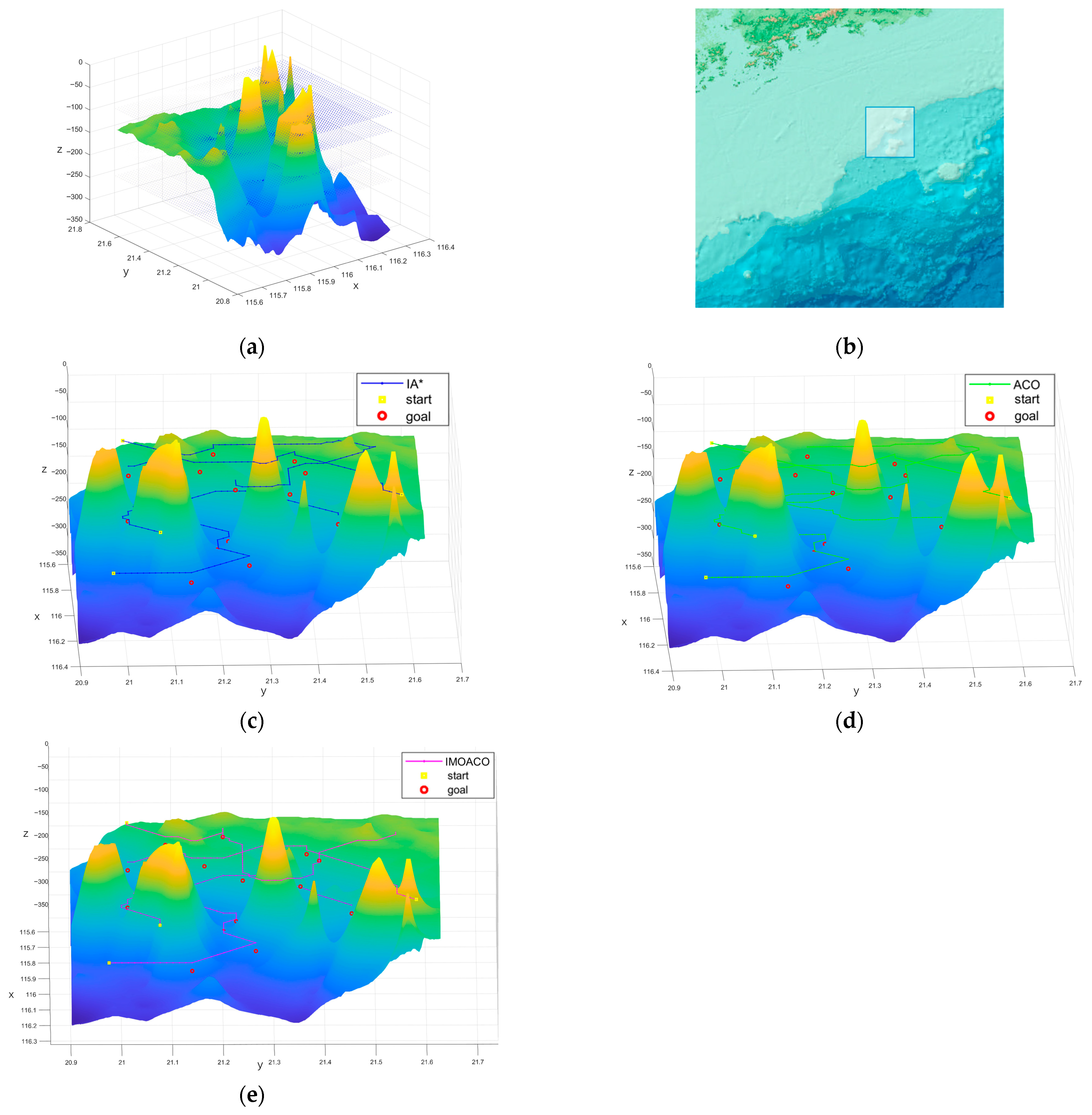
To verify the performance of the IMOACO algorithm, the present simulation introduces a marine environment constructed from GEBCO data, with comparisons made against the ACO and IA* algorithms. The test area lies within longitude E 115.6–116.3° and latitude N 20.9–21.63°, covering approximately 81 km × 73 km, with a grid resolution of 100 m as shown in Figure 12a. For clarity of presentation, current information is not displayed in the figure. Target points are randomly distributed within each layer. Based on the detection performance of forward-looking sonar, targets in the three-dimensional space are divided into four layers according to vertical distance and projected onto a 2D grid map. Simulation results are presented in Figure 12, and a comparison of metrics for the three algorithms is provided in

Table 7. Comparison of various metrics for three algorithms in the second simulation.

Algorithm	Length (m)	Energy Consumption (J)	Turning Angle (°)	Duration (s)
IA*	734,160.21	4,284,407.52	3420	423,505.61
ACO	738,177.43	4,299,755.26	4815	425,056.26
IMOACO	622,100.46	3,473,920.53	3285	343,390.44

.

Comparative results in Table 7 demonstrate that IMOACO achieves superior overall performance in multi-objective path planning. The algorithm yields a path length of 622,100.46 m, representing reductions of 15.27% and 15.74% compared to the IA* and ACO algorithms, respectively. Energy consumption reaches 3,473,920.53 J, showing decreases of 18.9% and 20.1% relative to IA* and ACO. The total turning angle is 3285°, corresponding to reductions of 4.0% and 31.7% compared to IA* and ACO, respectively, indicating significantly improved path smoothness. The task duration is 343,390.44 s, shortened by 18.9% and 20.7% compared to IA* and ACO. These simulation results validate both the effectiveness and engineering applicability of the IMOACO algorithm in ocean current environments.

5. Field Testing of the “Xinghai 300R” AUV

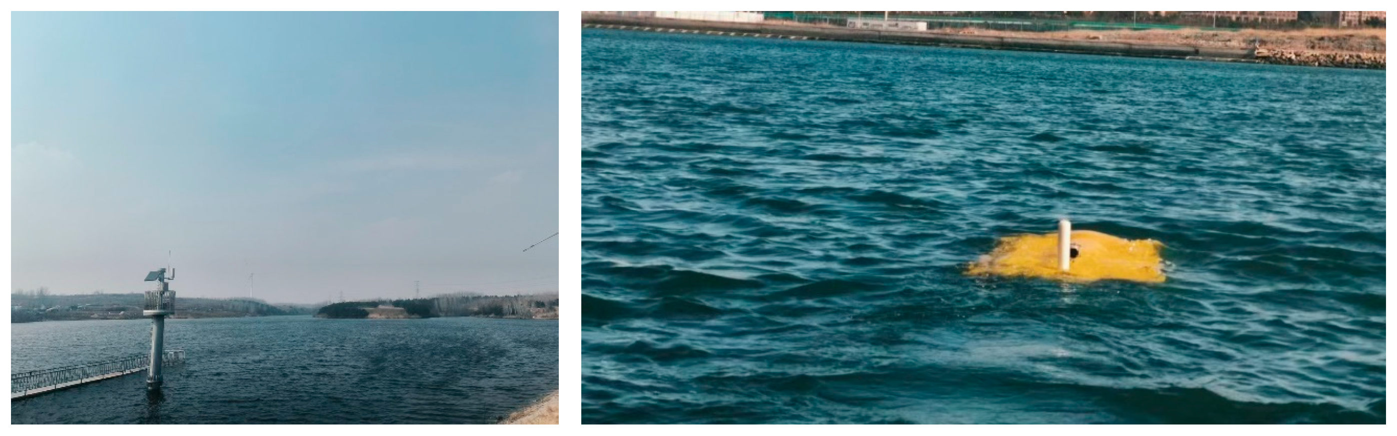
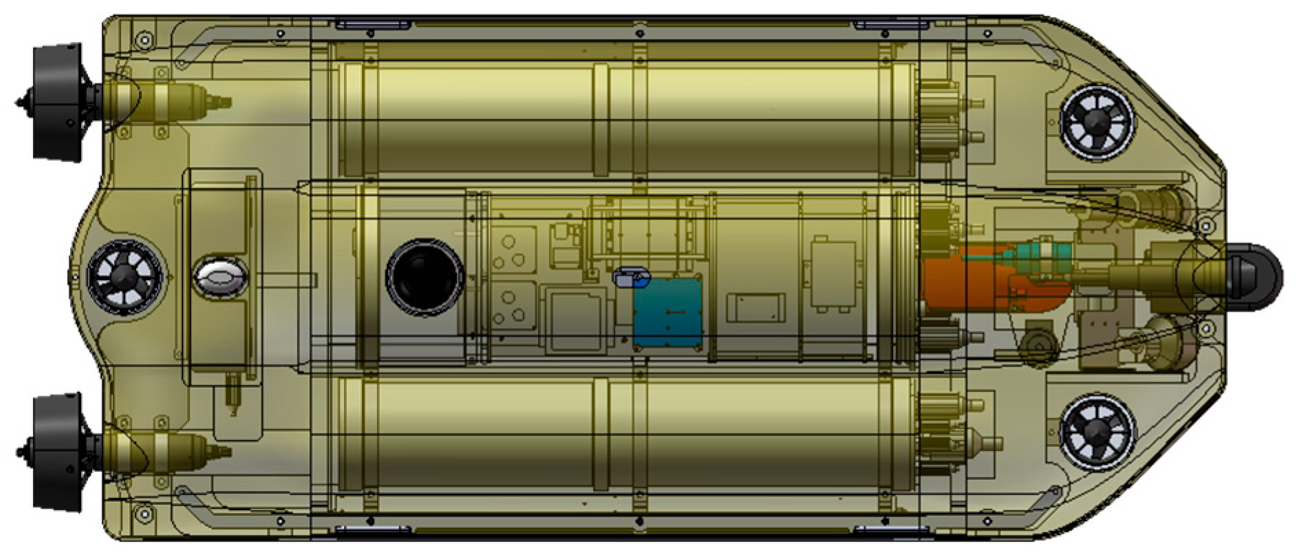
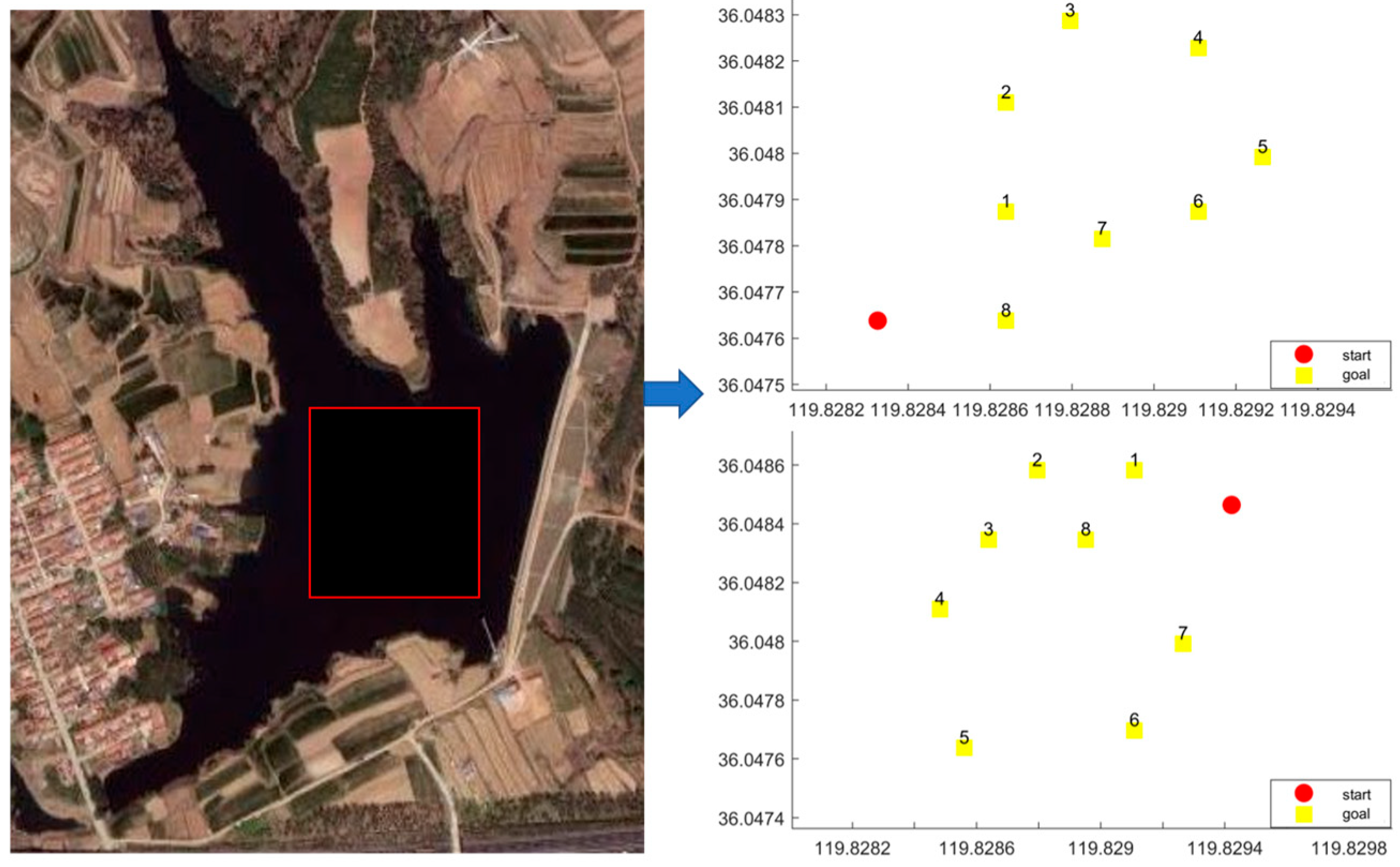
To verify the practical performance of the proposed IMOACO path planning method, it was implemented on the “Xinghai 300R” AUV (Harbin Engineering University, Harbin, Heilongjiang Province, China) for field experiments. As shown in Figure 13, the “Xinghai 300R” AUV employs a propulsion configuration comprising three vertical thrusters and two main thrusters. This setup enables three-dimensional omnidirectional maneuverability with a maximum speed of 2 m/s. The IMOACO algorithm prioritizes path smoothness as a core optimization objective, aiming to ensure coherent AUV motion by minimizing unnecessary turns. This approach effectively reduces energy consumption during navigation and shortens overall mission duration. Therefore, when validating the IMOACO algorithm using the actual vessel, only the speed constraint needs to be considered. Surface operation mode was adopted to minimize errors caused by underwater navigation inaccuracies. The test was conducted at the Qingdao Jinshaogou Reservoir, within the longitudinal range of E 119.828169–119.829735° and the latitudinal range of N 36.047520–36.048700°, covering a rectangular area of approximately 140 m × 140 m, as shown in Figure 14. The experiment included two comparative trials with eight target points randomly deployed in the test area; their specific distribution is illustrated in Figure 15.

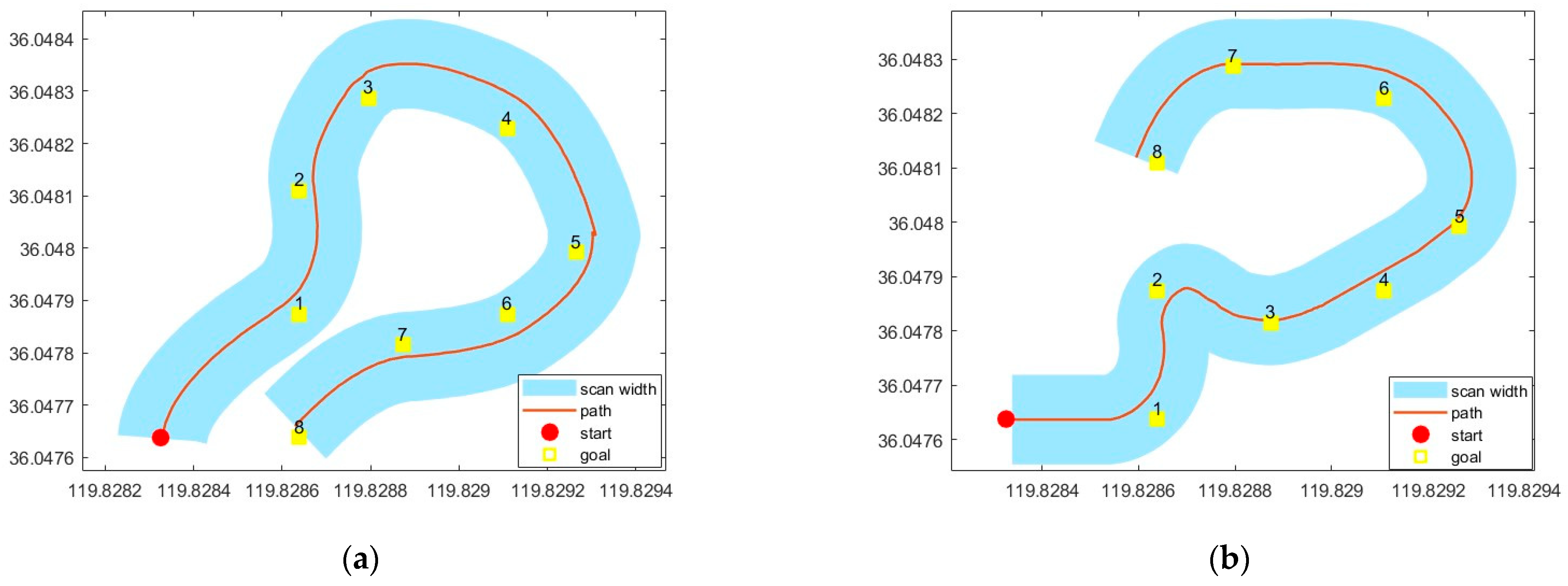
This experiment compares the performance of the IMOACO algorithm with the conventional ACO algorithm in multi-target path traversal. After generating optimal visitation sequences through each algorithm, the AUV follows the planned path to visit all target points sequentially. During testing, some trajectories deviated significantly from the target point. This was primarily caused by the coupling of positioning accuracy errors and the set pass-over radius. However, the effective detection range of the AUV’s forward-looking sonar exceeded this deviation, enabling target point detection. The current sea current vector measured by ADCP (Acoustic Doppler Current Profiler) represents the average horizontal flow velocity within the test area. As the experiment was conducted in a reservoir environment, the flow field is primarily dominated by wind-generated currents. Spatial variations are relatively gradual, with no significant vortex structures observed, allowing the flow field to be considered constant and static. The water flow vector in Scenario 1 is (–0.3, –0.3), with the actual navigation track shown in Figure 16.

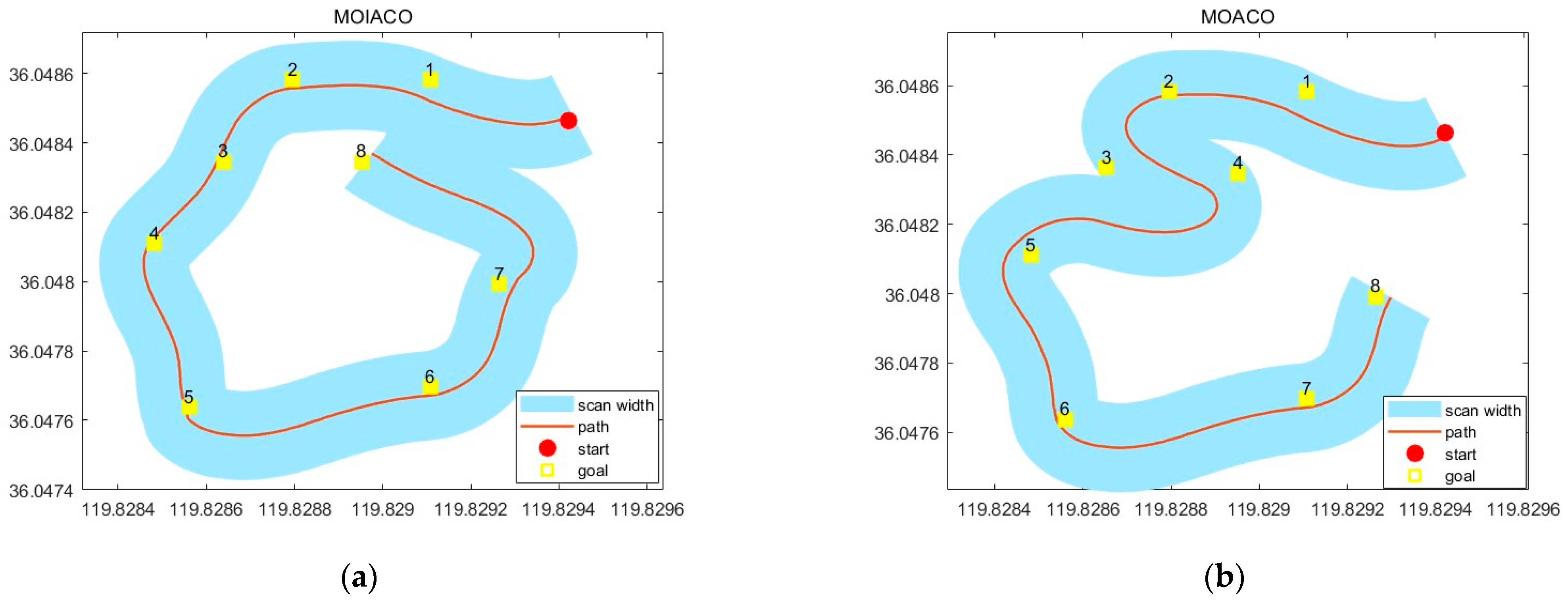
Experimental results indicate that the IMOACO algorithm demonstrates improved motion optimization characteristics in path planning (see Figure 16a). Compared with the path generated by the conventional ACO algorithm (see Figure 16b), IMOACO achieves better trajectory smoothness, owing to its multi-objective optimization mechanism. The conventional ACO approach, which uses path length as the sole objective, tends to select the nearest local nodes during multi-target traversal, leading to redundant turns. This not only increases travel through counter-current segments and non-linear energy consumption, but also prolongs the mission duration. Quantitative results (

Table 8. Comparison of various metrics for two algorithms in the first field trial.

Algorithm	Length (m)	Energy Consumption (J)	Turning Angle (°)	Duration (s)
IMOACO	331.64	249.38	1022.52	665.56
ACO	315.73	259.21	1091.34	691.79

) show that although the path length of IMOACO is 5.0% longer than that of ACO, it reduces energy consumption by 3.78%; the number of turns is reduced by 6.3%, and the total mission time is reduced by 3.79%. To examine the robustness of the algorithm, multiple additional experiments were conducted. A comparative experiment was carried out under a current vector of (0.21, 0.22) with repositioned target points. The resulting paths are presented in Figure 17.

As shown in the Figure 17, the path generated by the IMOACO algorithm demonstrates high smoothness with minimal turning angles between target points. In contrast, the path in Figure 17b exhibits larger turning angles, leading to increased energy consumption and reduced mission duration. According to

Table 9. Comparison of various metrics for two algorithms in the second field trial.

Algorithm	Length (m)	Energy Consumption (J)	Turning Angle (°)	Duration (s)
IMOACO	220.86	182.51	963.12	487.10
ACO	202.84	184.33	1003.49	491.96

, the path length of IMOACO increases by 8.9% compared to ACO, while energy consumption decreases by 1.0%, the turning angle is reduced by 4.0%, and mission duration is shortened by 0.99%.

In conclusion, the IMOACO algorithm exhibits superior energy consumption control, heading stability, and mission efficiency by effectively utilizing ocean current characteristics, validating its effectiveness and engineering applicability for multi-target search and rescue operations in complex ocean current environments.

6. Discussion

The design of the IMOACO algorithm effectively addresses the limitations inherent in conventional path planning when applied to complex marine settings. This is achieved through a novel fusion of environmental dynamic principles and multi-objective optimization theory. The algorithm establishes a current-oriented decision mechanism coupled with an adaptive framework for balancing multiple optimization criteria.

Conventional approaches typically treat ocean currents as constraints in path planning. In contrast, the IMOACO algorithm incorporates a heading–current angle heuristic function, transforming current vectors into favorable factors during path search. This interactive planning strategy, grounded in environmental awareness, allows the algorithm to identify and exploit downstream paths, thereby significantly improving energy efficiency. The velocity composition relationship illustrated in Figure 2 provides a physical basis for this mechanism, quantifying the interaction between the current vector and the navigation direction, and supporting the computation of state transition probabilities.

In the field of multi-objective optimization, the entropy weight method facilitates a significant shift from subjective to objective weighting. This data-driven approach adaptively adjusts the relative importance of each evaluation metric based on the statistical characteristics of environmental data, thereby overcoming the limitations of fixed-weight strategies in complex and dynamic environments.

The computational complexity of IMOACO is determined by the target point pairs and the TSP problem iterations, influenced by parameters such as the number of target points, maximum iteration count, ant population size, and map grid scale. The algorithm’s complexity is $O({10}^9)$, enabling minute-level computation. Second-level computation remains challenging to achieve under current hardware limitations. Therefore, this algorithm is currently suitable for offline planning of small-scale tasks and larger-scale tasks where real-time requirements do not demand sub-second performance. For applications requiring higher real-time performance, computation time can be reduced to the 10-s range by decreasing the number of iterations, reducing the number of ants, implementing parallel processing, or adopting an incremental update strategy.

However, current research still exhibits certain limitations. To address the current limitation in field validation tasks that restricts the scale of experiments, resulting in limited performance improvements in quantitative comparisons, we will prioritize advancing large-scale field validation in future work. This will enable a more comprehensive assessment of the IMOACO algorithm’s performance in real ocean environments. Transitioning the test environment to long-term uncertain flow fields may trigger multidimensional fluctuations in the IMOACO algorithm’s performance: path stability, energy efficiency, and convergence all face challenges. However, the algorithm’s core innovation provides a foundation for adaptive improvements—by integrating real-time perception and optimizing weight update frequency, IMOACO can be extended to more realistic ocean environments. Future work should focus on flow-algorithm coupled simulations, combined with long-term field testing using the “Xinghai 300R” AUV, to further enhance the algorithm’s engineering robustness under uncertain conditions. Furthermore, while the layered projection strategy employed in 3D path planning reduces computational complexity, it does not fully incorporate the AUV’s kinematic constraints in the vertical dimension, such as pitch and buoyancy control.

Future research should prioritize dynamic environment modeling and online replanning capabilities, integrated planning-control co-design, and comprehensive 3D path optimization. These advancements are crucial for enhancing the algorithm’s adaptability and robustness in complex and uncertain ocean environments. While the current study focuses on metaheuristic comparisons to address the real-time requirements and environmental uncertainties in AUV rescue missions, future work will further extend the theoretical completeness by incorporating exact method benchmarks in controlled static scenarios. This extension will quantitatively evaluate the optimality gap of IMOACO, thereby reinforcing its theoretical robustness without compromising the practical relevance validated in this study.

7. Conclusions

This study focuses on the challenges of inefficient path planning and weak disturbance resistance for rescue AUVs in complex ocean environments, systematically conducting research on the design and validation of path optimization algorithms. To overcome the limitations of conventional methods, which insufficiently consider dynamic ocean current interference and lack robust obstacle avoidance, an IMOACO algorithm is proposed. The effectiveness of the algorithm is thoroughly validated through simulation analysis and field tests with an actual AUV. The main research findings are summarized as follows:

(1)

A flow-driven objective function and state transition function are developed, incorporating multidimensional evaluation metrics including path length, energy consumption, and smoothness. By introducing a current-aware mechanism and designing a dynamic pheromone update strategy, the algorithm’s adaptability to oceanic current disturbances is significantly enhanced.

(2)

An ocean current-guided IMOACO algorithm is established for large-scale multi-target search and rescue missions. The approach synthesizes path length, energy consumption, and smoothness into a multi-objective heuristic evaluation model, while an adaptive pheromone evaporation mechanism improves convergence efficiency and stability.

(3)

Through simulations and field tests using the “Xinghai 300R” AUV, the IMOACO algorithm demonstrates improvements of 15.27% in path length, 18.9% in energy consumption, and 31.7% in path turning angle compared to IA* and ACO algorithms, with a 20.7% enhancement in mission efficiency. These results validate the algorithm’s robustness and engineering practicality for multi-target operations in complex ocean current environments.

In summary, the IMOACO algorithm proposed in this study significantly improves both the mission efficiency and path quality of rescue AUVs operating in complex, dynamic marine environments, demonstrating substantial theoretical value and promising application prospects. Future work will focus on high-precision dynamic environment modeling, multi-source perception fusion, and intelligent control mechanisms, aiming to advance underwater rescue equipment toward higher levels of intelligence and autonomy. These research directions will provide solid technical support for marine emergency response and resource assurance operations.

References

1. Zhou, N.; Zhu, Z.; Mu, X.; Zhou, L.; Qin, H.; Bai, G. Hybrid-Algorithm-Based Emergency Search and Rescue Method with AUV to Uncertain Environment in Internet of Underwater Things. IEEE Internet Things J. 2025, 12, 29925–29939. [Google Scholar] [CrossRef]
2. Zhou, J.; Si, Y.; Chen, Y. A Review of Subsea AUV Technology. J. Mar. Sci. Eng. 2023, 11, 1119. [Google Scholar] [CrossRef]
3. Cai, C.; Chen, J.; Ayub, M.S.; Liu, F. A Task Allocation Method for Multi-AUV Search and Rescue with Possible Target Area. J. Mar. Sci. Eng. 2023, 11, 804. [Google Scholar] [CrossRef]
4. Cheng, C.; Sha, Q.; He, B.; Li, G. Path Planning and Obstacle Avoidance for AUV: A Review. Ocean Eng. 2021, 235, 109355. [Google Scholar] [CrossRef]
5. Wang, L.; Zhu, D.; Pang, W.; Zhang, Y. A Survey of Underwater Search for Multi-Target Using Multi-AUV: Task Allocation, Path Planning, and Formation Control. Ocean Eng. 2023, 278, 114393. [Google Scholar] [CrossRef]
6. Guo, Y.; Liu, H.; Fan, X.; Lyu, W. Research Progress of Path Planning Methods for Autonomous Underwater Vehicle. Math. Probl. Eng. 2021, 2021, 8847863. [Google Scholar] [CrossRef]
7. Wang, Y.; Zheng, Y.R. 3-Dimensional Path Planning for Autonomous Underwater Vehicle. In Proceedings of the OCEANS 2018 MTS/IEEE Charleston, Charleston, SC, USA, 22–25 October 2018; pp. 1–6. [Google Scholar] [CrossRef]
8. Yazdani, A.M.; Sammut, K.; Lammas, A.; Tang, Y. Real-Time Quasi-Optimal Trajectory Planning for Autonomous Underwater Docking. In Proceedings of the 2015 IEEE International Symposium on Robotics and Intelligent Sensors (IRIS), Langkawi, Malaysia, 18–20 October 2015; pp. 15–20. [Google Scholar] [CrossRef]
9. Wolek, A.; McMahon, J.; Dzikowicz, B.R.; Houston, B.H. The Orbiting Dubins Traveling Salesman Problem: Planning Inspection Tours for a Minehunting AUV. Auton. Robots 2021, 45, 31–49. [Google Scholar] [CrossRef]
10. Sun, B.; Zhang, W.; Li, S.; Zhu, X. Energy Optimised D* AUV Path Planning with Obstacle Avoidance and Ocean Current Environment. J. Navig. 2022, 75, 685–703. [Google Scholar] [CrossRef]
11. Garau, B.; Alvarez, A.; Oliver, G. Path Planning of Autonomous Underwater Vehicles in Current Fields with Complex Spatial Variability: An A* Approach. In Proceedings of the 2005 IEEE International Conference on Robotics and Automation, Barcelona, Spain, 18–22 April 2005; pp. 194–198. [Google Scholar] [CrossRef]
12. Zeng, Z.; Lammas, A.; Sammut, K.; He, F.; Tang, Y. Shell Space Decomposition Based Path Planning for AUVs Operating in a Variable Environment. Ocean Eng. 2014, 91, 181–195. [Google Scholar] [CrossRef]
13. Yan, Z.; Zhao, Y.; Zhang, H. A Method of UUV Path Planning with Biased Extension in Ocean Flows. In Proceedings of the Proceedings of the 10th World Congress on Intelligent Control and Automation, Beijing, China, 6–8 July 2012; pp. 532–537. [Google Scholar] [CrossRef]
14. Zeng, Z.; Sammut, K.; Lian, L.; He, F.; Lammas, A.; Tang, Y. A Comparison of Optimization Techniques for AUV Path Planning in Environments with Ocean Currents. Robot. Auton. Syst. 2016, 82, 61–72. [Google Scholar] [CrossRef]
15. Khan, M.T.R.; Ahmed, S.H.; Jembre, Y.Z.; Kim, D. An Energy-Efficient Data Collection Protocol with AUV Path Planning in the Internet of Underwater Things. J. Netw. Comput. Appl. 2019, 135, 20–31. [Google Scholar] [CrossRef]
16. Vinoth Kumar, S.; Jayaparvathy, R.; Priyanka, B.N. Efficient Path Planning of AUVs for Container Ship Oil Spill Detection in Coastal Areas. Ocean. Eng. 2020, 217, 107932. [Google Scholar] [CrossRef]
17. Guo, X.; Ji, M.; Zhao, Z.; Wen, D.; Zhang, W. Global Path Planning and Multi-Objective Path Control for Unmanned Surface Vehicle Based on Modified Particle Swarm Optimization (PSO) Algorithm. Ocean Eng. 2020, 216, 107693. [Google Scholar] [CrossRef]
18. Mao, Y.; Pang, Y. Application of improved particle swarm optimization in path planning of underwater vehicles: Application of improved particle swarm optimization in path planning of underwater vehicles. J. Comput. Appl. 2010, 30, 789–792. [Google Scholar] [CrossRef]
19. Zhang, G.; Liu, J.; Sun, Y.; Ran, X.; Chai, P. Research on AUV Energy Saving 3D Path Planning with Mobility Constraints. J. Mar. Sci. Eng. 2022, 10, 821. [Google Scholar] [CrossRef]
20. Liang, S.; Zhi-ming, Q.; Heng, L. A Survey on Route Planning Methods of AUV Considering Influence of Ocean Current. In Proceedings of the 2018 IEEE 4th International Conference on Control Science and Systems Engineering (ICCSSE), Wuhan, China, 21–23 August 2018; pp. 288–295. [Google Scholar] [CrossRef]
21. Chen, X.; Kong, Y.; Fang, X.; Wu, Q. A Fast Two-Stage ACO Algorithm for Robotic Path Planning. Neural Comput. Appl. 2013, 22, 313–319. [Google Scholar] [CrossRef]
22. Duan, H.; Yu, Y.; Zhang, X.; Shao, S. Three-Dimension Path Planning for UCAV Using Hybrid Meta-Heuristic ACO-DE Algorithm. Simul. Model. Pract. Theory 2010, 18, 1104–1115. [Google Scholar] [CrossRef]
23. Li, G.; Liu, C.; Wu, L.; Xiao, W. A Mixing Algorithm of ACO and ABC for Solving Path Planning of Mobile Robot. Appl. Soft Comput. 2023, 148, 110868. [Google Scholar] [CrossRef]
24. Chen, Y.; Bai, G.; Zhan, Y.; Hu, X.; Liu, J. Path Planning and Obstacle Avoiding of the USV Based on Improved ACO-APF Hybrid Algorithm With Adaptive Early-Warning. IEEE Access 2021, 9, 40728–40742. [Google Scholar] [CrossRef]
25. Aghababa, M.P.; Amrollahi, M.H.; Borjkhani, M. Application of GA, PSO, and ACO Algorithms to Path Planning of Autonomous Underwater Vehicles. J. Mar. Sci. Appl. 2012, 11, 378–386. [Google Scholar] [CrossRef]
26. Yi, G.; Feng-ting, Q.; Fu-jia, S.; Wei-ming, H.; Peng-ju, Z. Research on Path Planning for Mobile Robot Based on ACO. In Proceedings of the 2017 29th Chinese Control And Decision Conference (CCDC), Chongqing, China, 28–30 May 2017; pp. 6738–6743. [Google Scholar] [CrossRef]
27. Yu, Y.; Zheng, H.; Xu, W. Learning and Sampling-Based Informative Path Planning for AUVs in Ocean Current Fields. IEEE Trans. Syst. Man Cybern Syst. 2025, 55, 51–62. [Google Scholar] [CrossRef]
28. Nazarahari, M.; Khanmirza, E.; Doostie, S. Multi-Objective Multi-Robot Path Planning in Continuous Environment Using an Enhanced Genetic Algorithm. Expert Syst. Appl. 2019, 115, 106–120. [Google Scholar] [CrossRef]
29. Ajeil, F.H.; Ibraheem, I.K.; Sahib, M.A.; Humaidi, A.J. Multi-Objective Path Planning of an Autonomous Mobile Robot Using Hybrid PSO-MFB Optimization Algorithm. Appl. Soft Comput. 2020, 89, 106076. [Google Scholar] [CrossRef]
30. Liu, C.; Mao, Q.; Chu, X.; Xie, S. An Improved A-Star Algorithm Considering Water Current, Traffic Separation and Berthing for Vessel Path Planning. Appl. Sci. 2019, 9, 1057. [Google Scholar] [CrossRef]
31. Chaari, I.; Koubaa, A.; Bennaceur, H.; Trigui, S.; Al-Shalfan, K. smartPATH: A Hybrid ACO-GA Algorithm for Robot Path Planning. In Proceedings of the 2012 IEEE Congress on Evolutionary Computation, Brisbane, Australia, 10–15 June 2012; pp. 1–8. [Google Scholar] [CrossRef]
Figure 1. Ocean current environment.
Jmse 14 00013 g001
Figure 2. The composite relationship of V A , V w , V s in p i : (a) the angle is acute; (b) the angle is obtuse.
Jmse 14 00013 g002
Figure 3. Path corner.
Jmse 14 00013 g003
Figure 4. Convergence process and standard deviation variation of three weighting coefficients: (a) path length weighting coefficient; (b) energy consumption weighting coefficient; (c) turning angle weighting coefficient; (d) standard deviation variation of the three weighting coefficients.
Jmse 14 00013 g004
Figure 5. Schematic diagram of the proportion in the iterative process of three weighting coefficients.
Jmse 14 00013 g005
Figure 6. IMOACO algorithm flowchart.
Jmse 14 00013 g006
Figure 7. Simulation results for different cost functions.
Jmse 14 00013 g007
Figure 8. Statistical results of the experiment, the lines in the figure are error bars, representing the dispersion of this set of data: (a) path lengths comparison across different algorithms; (b) energy consumption comparison of different algorithms; (c) corner comparison across different algorithms; (d) duration comparison of different algorithms.
Jmse 14 00013 g008
Figure 9. Simulation of path planning for three different algorithms under six random ocean current scenarios.
Jmse 14 00013 g009
Figure 10. Comparison of IMOACO paths in complex environments: (a) fixed weights; (b) adaptive weights.
Jmse 14 00013 g010
Figure 11. Simulation of multi-objective algorithm in GEBCO-generated terrain environment: (a) satellite image; (b) multi-object detection simulations of three algorithms.
Jmse 14 00013 g011
Figure 12. Comprehensive simulation of three algorithms: (a) processed environment data; (b) map data generated via GEBCO; (c) multi-objective simulation 3D view of IA*-GA algorithm; (d) multi-objective simulation 3D view of traditional ACO algorithm; (e) multi-objective simulation 3D view of IMOACO algorithm.
Jmse 14 00013 g012
Figure 13. Structural Diagram of the “Xinghai 300R” AUV.
Jmse 14 00013 g013
Figure 14. Test site and “Xinghai 300R” AUV.
Jmse 14 00013 g014
Figure 15. Satellite image of the test site and multiple target points.
Jmse 14 00013 g015
Figure 16. Multi-objective path planning for scenario 1: (a) IMOACO; (b) ACO.
Jmse 14 00013 g016
Figure 17. Multi-objective path planning for scenario 2: (a) IMOACO; (b) ACO.
Jmse 14 00013 g017