Automated Machine Learning-Based Significant Wave Height Prediction for Marine Operations

Abstract

Determining/predicting the environment dominates a variety of marine operations, such as route planning and offshore installation. Significant wave height (Hs) is a critical parameter-defining wave, a dominating marine load. Data-driven machine learning methods have been increasingly applied to Hs prediction, but challenges remain in hyperparameter tuning and spatial generalization. This study explores a novel effective approach for intelligent Hs forecasting for marine operations. Multiple automated machine learning (AutoML) frameworks, namely H2O, PyCaret, AutoGluon, and TPOT, have been systematically evaluated on buoy-based Hs prediction tasks, which reveal their advantages and limitations under various forecast horizons and data quality scenarios. The results indicate that PyCaret achieves superior accuracy in short-term forecasts, while AutoGluon demonstrates better robustness in medium-term and long-term predictions. To address the limitations of single-point prediction models, which often exhibit high dependence on localized data and limited spatial generalization, a multi-point data fusion framework incorporating Principal Component Analysis (PCA) is proposed. The framework utilizes Hs data from two stations near the California coast to predict Hs at another adjacent station. The results indicate that it is possible to realize cross-station predictions based on the data from adjacent (high relevance) stations.

1. Introduction

A wave is one of the most important marine dynamic loads [1]. Significant wave height (Hs) is the core parameter-defining wave and is of key significance for the safety of floating structures and marine operations [2]. With the rapid development of offshore oil and gas, renewable energy (e.g., wind and wave), and marine transportation, demands on Hs prediction for the industries are growing fast [3]. Hs predictions are of great value for marine operation decision-making (e.g., window selection) and ship route optimization. Currently, Hs prediction can be divided into numerical simulation based on physical formulations and data-driven machine learning methods.

Wave models based on physical equations are the traditional method for wave height prediction [4]. These models simulate the temporal and spatial evolution of ocean waves based on meteorological wind fields, ocean dynamics equations, and source–sink term parameterizations [5]. They are grounded in solid theoretical foundations and capable of characterizing complex processes such as wind-wave generation, energy balance, and nonlinear wave breaking [6]. However, wave models based on physical equations require prolonged computation times at high resolution grids [7]. These numerical wave models especially face great challenges due to significant uncertainties in the initial conditions and their high sensitivity to the boundary conditions [8,9]. Under extreme weather conditions, e.g., the Draupner rogue wave event in 1995 [10], they still face challenges in terms of applicability and stability [11,12].

Data-driven machine learning (ML) methods are gaining attention [13] for wave height prediction. By analyzing wave observation data (e.g., buoy observations, remote sensing, reanalysis products), ML models can directly predict significant wave height by learning mapping relationships in historical time series data [14]. Unlike purely physics-based models, ML avoids solving complex wave dynamics equations, offering advantages in computational speed and accuracy for specific scenarios [15]. Neural networks (NNs), support vector machines (SVMs), random forests (RFs), and long short-term memory networks (LSTM) are widely used in Hs prediction [16,17]. Among them, deep learning (DL) particularly excels at capturing multidimensional/nonlinear features. Several studies have verified that its prediction accuracy is similar to or even better than that of wave models based on physical equations [18,19].

However, traditional ML/DL models still face challenges in feature engineering, model architecture, and hyperparameter tuning [20]. Hyperparameters are non-trainable parameters determining preprocessing, model structure, and processing procedure, and they have significant influences on performance [21]. In addition, different sea areas, observation data scales, or extreme sea conditions can cause significant differences. Researchers usually need to conduct many trials to find the optimal model configuration. Automated hyperparameter optimization (HPO) methods provide an efficient alternative to time-consuming manual trials for identifying optimal configurations [22]. Pirhooshyaran et al. [23] integrated Bayesian HPO with elastic networks within a recurrent neural network framework, yielding improved model resilience through comparative analysis. Similarly, by integrating Fourier neural operators and hyperparameter search into data-driven ocean modeling, Sun et al. [24] improved single-time-step prediction accuracy.

On top of these progresses, automated machine learning (AutoML) techniques have emerged in recent years. AutoML aims to automate feature selection, model selection, hyperparameter tuning, and end-to-end workflows, significantly reducing manual intervention and requirements for user expertise. The Auto-sklearn framework developed by Feurer et al. [25] and the systematic approach proposed by Hutter et al. [26] laid the theoretical and practical foundations of AutoML. This concept provides a new solution for ocean and weather modeling with high complexity and data diversity. AutoML has gained increasing attention in the ocean and weather fields in recent years [27]. By employing automated search strategies for model selection, feature engineering, and hyperparameter optimization [28], AutoML reduces reliance on human expertise while accelerating model deployment cycles [29]. Various studies indicate its effectiveness in wave prediction [30]. However, its prediction accuracy, computational efficiency, and generalization in dynamic marine environments remain to be explored systematically.

The intercorrelation of ocean waves in spatial distribution is also an important input factor in Hs prediction [31]. The wave characteristics at different geographical locations within the sea area are often influenced by common factors such as wind fields, topography, and ocean currents [32]. Single-point prediction for Hs only inputs in situ data and cannot utilize other location data to improve the robustness and accuracy of the overall prediction [33]. These models also tend to overfit and generalize poorly in data-scarce/heterogeneous marine environments [34].

To address the limitations of the single-point prediction paradigm, multi-point data fusion has emerged as a robust strategy. By incorporating data from multiple observation points during the model training phase, this approach maximizes the utilization of both common and differential characteristics across various geographical locations within the sea area [35]. Prior studies have demonstrated that multi-point data fusion significantly enhances the model’s generalization capability for new observation points with incomplete data. Additionally, it exhibits greater adaptability in response to variations in ocean waves across different spatiotemporal scales [36].

Therefore, considering the limitations in Hs prediction, this paper conducts studies from two primary perspectives. First, the performance of mainstream AutoML algorithms has been systematically evaluated for Hs forecasting, providing a comprehensive comparison of their practical effectiveness in wave prediction. Second, a multi-point data fusion framework that leverages spatial correlations between locations to enhance the model’s spatial generalization capabilities is proposed. The results demonstrate that AutoML can significantly reduce manual hyperparameter tuning efforts and that multi-point data fusion provides a feasible way to reduce the dependency of single-point models on localized environmental conditions. The structure of this paper is listed below. Section 2 details the data sources and selected AutoML algorithms. Section 3 compares results from four AutoML models, analyzing their performance and robustness. Section 4 illustrates the spatial generalization of the data fusion model. Finally, Section 5 is the summary and further discussion.

2. Materials and Methods

2.1. Data Sources

Data-driven machine learning requires high-quality and reliable data for training. Satellite remote sensing data, numerical reanalysis information, and buoy-measured data are the three main data sources for acquiring Hs data. In this study, buoy-measured data from the U.S. National Data Buoy Center (NDBC) are used (data accessed from https://www.ndbc.noaa.gov).

NDBC data were selected because buoy in situ observations provide more authentic representations of raw wave dynamics (satellite altimeters and reanalysis products may introduce biases through post-processing algorithms). Five NDBC stations were ultimately chosen, 42095, 46239, 46047, 41049, and 46028, with their geographical distribution visualized in Figure 1. The selection of buoys considered geospatial distribution (e.g., varied water depths) and data quality (low missing-value rates) [34].

Each buoy site is analyzed as an independent research object (utilizing its own Hs time series only) and the dataset has a 1 h temporal resolution. Missing values in raw data are retained without imputation to preserve the originality of the dataset. The geographic location identifiers (ID) of the sites and their statistical characteristics (maximum, mean, variance, etc.) are detailed in

Table 1. Location identifiers and Hs statistical characteristics of the buoy sites.

ID	Location	Site Code	Count	Mean (m)	Max (m)	Min (m)	Std (m)	Depth (m)
1	(24°24′31″ N, 81°58′3″ W)	42095	24,396	0.734	7.5	0.1	0.440	100
2	(36°20′5″ N, 122°6′14″ W)	46239	23,111	2.200	8.42	0.52	0.917	369
3	(32°25′6″ N, 119°32′6″ W)	46047	25,365	2.100	8.31	0.59	0.827	1423
4	(27°30′17″ N, 62°16′14″ W)	41049	25,944	1.793	7.96	0.61	0.832	5480
5	(35°46′12″ N, 121°54′11″ W)	46028	25,139	2.241	8.78	0.48	0.906	1154

.

In the subsequent contents, a hierarchical validation strategy is adopted. The data of buoys ID1–ID4 are used for the side-by-side comparison of the AutoML algorithm. Hs data of buoys ID2 and ID3 are fused in feature space to construct an extended training set with cross-station features. The buoy ID5 is used to verify the model’s extrapolation prediction performance. This hierarchical validation not only evaluates the model’s prediction on point-specific Hs, but also examines its generalization performance on heterogeneous data.

This study uses a consistent data split strategy across all AutoML frameworks. For each buoy site, data from January 2021 to December 2023 is sorted in chronological order. The first 80% of the samples serve as the training set (used for both model training and validation), and the remaining 20% constitute the test set (used solely for final evaluation). The test set is positioned strictly after the training set in time to prevent any potential data leakage.

2.2. Automated Machine Learning

A variety of AutoML algorithms have been developed. These tools vary in terms of search algorithms, model integration strategies, and hardware acceleration.

Table 2. Comparison of four automated machine learning tools.

Tool	Search Algorithm	Ensemble Strategy	Acceleration Support
TPOT	Genetic Algorithm + Tree-based Pipeline Optimization	Best Model Only	CPU-only
H2O	Cartesian Grid + Random Search	Stacked Ensembles	GPU Support
AutoGluon	Bayesian Optimization	Multi-model Stacking + Bagging	Native GPU
PyCaret	Random Search + Custom Search Space	Manual Selection	Limited GPU Support

compares several mainstream AutoML tools.

(1)

H2O

H2O is a distributed machine learning platform [37] developed to streamline the machine learning pipeline from data preprocessing to model deployment. Unlike traditional AutoML tools that mainly concentrate on model selection and hyperparameter tuning, H2O integrates comprehensive functionalities including missing value imputation, categorical variable encoding, feature scaling, and ensemble modeling. It features a parallel training system covering widely used algorithms such as GLM, random forest XGBoost, and deep learning. Additionally, H2O applies stacked ensemble techniques to combine the strengths of multiple models, which often leads to more stable and accurate predictions. Its flexibility allows it to handle various tasks like classification, regression, and anomaly detection efficiently, making it suitable for both academic research and industry applications. The experiments adopt H2O version 3.44.0.3, with computations performed using PyCharm Professional 2022.1.3.

(2)

PyCaret

PyCaret streamlines machine learning workflows through its modular packaging [38]. Its core strengths lie in automated feature engineering and cross-framework integration capabilities. For time series data, the library’s built-in time series feature generator automatically creates lagged features (e.g., historical wave heights from moment’s t-1 to t-3). It can reject highly correlated redundant variables through Pearson correlation coefficient thresholding. The model training phase adopts a hybrid optimization strategy. This approach integrates Bayesian optimization with grid search to jointly tune hyperparameters for algorithms including LightGBM and CatBoost. The experiments are computed with PyCaret version 3.3.2.

(3)

AutoGluon

AutoGluon is an open source AutoML toolkit [39] proposed in 2020. Compared with traditional AutoML, which focuses on algorithm selection and hyperparameter optimization, AutoGluon mainly improves raw data processing and multi-layer model integration. AutoGluon has high-level automation and is able to automatically perform tasks such as feature engineering, model selection, and hyperparameter tuning. AutoGluon supports many types of machine learning tasks, such as classification, regression, clustering, etc. Its robust training strategies integrate a variety of excellent machine learning algorithms, so AutoGluon can achieve great performance in a short time. The experiments in this study employ AutoGluon version 1.1.1.

(4)

TPOT

The Tree-based Pipeline Optimization Tool (TPOT) is a genetic programming-based optimizer that generates machine learning pipeline [40]. It extends the scikit learning framework with its own basic regressor and classifier methods. The TPOT innovatively introduces genetic programming to machine learning pipeline optimization by simulating the biological evolutionary process to automatically generate optimal workflows. The initial phase randomly generates 100 pipeline candidates, each candidate incorporating data preprocessing steps, feature transformation techniques, and regression models. Fitness evaluation is performed using a time series cross-validated weighted RMSE, while Pareto optimization is introduced to balance model accuracy and complexity. Experiments are run using the TPOT package (0.12.2) from Pycharm.

2.3. Evaluation Metrics

In this study, statistical methods are adopted to systematically evaluate model performance, validate prediction reliability, and provide quantitative support for the practical application of Hs forecasting. The statistical parameters used in the comparison include root mean square error (RMSE), mean absolute error (MAE), mean absolute percentage error (MAPE), Spearman correlation coefficient (SCC), and R-squared. RMSE is more sensitive to error magnitude, where lower values indicate better model fitting. Given $y_i$ as observed values, $y_T$ as predicted values, and n as sample size, the formula is defined as

$$\mathrm{RMSE}=\sqrt{{\displaystyle \frac{1}{n}}{\sum }_{i=1}^n {\left(y_i-y_T\right)}^2}$$

(1)

MAE is more inclusive of outliers than RMSE, and its formula is as follows:

$$\mathrm{MAE}= {\displaystyle \frac{1}{n}}{\sum }_{i=1}^n \left|\left(y_i-y_T\right)\right|$$

(2)

MAPE equals 0, meaning a perfect fitting, and the formula is as follows:

$$\mathrm{MAPE} = {\displaystyle \frac{1}{n}}{\sum }_{i=1}^n\left|{\displaystyle \frac{y_i-y_T}{y_i}}\right|$$

(3)

R-square takes the value in the range [–1, 1] (larger value represents better fitting), and the formula is as follows:

$$R^2 = 1-{\displaystyle \frac{SSE}{SST}} = 1-{\displaystyle \frac{\sum (y_T-y_i{)}^2}{\sum (y_i-\overline{y}{)}^2}}$$

(4)

SSE represents the sum of squares of the difference between the true value and the predicted value, and SST represents the sum of squares of the difference between the true data and its mean. The SCC takes the value in the range of [−1, 1], and larger value represents stronger temporal correlation between the two datasets. The formula is as follows:

$$\mathrm{SCC}= 1-{\displaystyle \frac{6\sum m_i^2}{n^3-n}}$$

(5)

Here, $m_i$ is the difference in the ranking of each pair of data in the two datasets.

3. Cross-Comparison of AutoML

3.1. Study Object

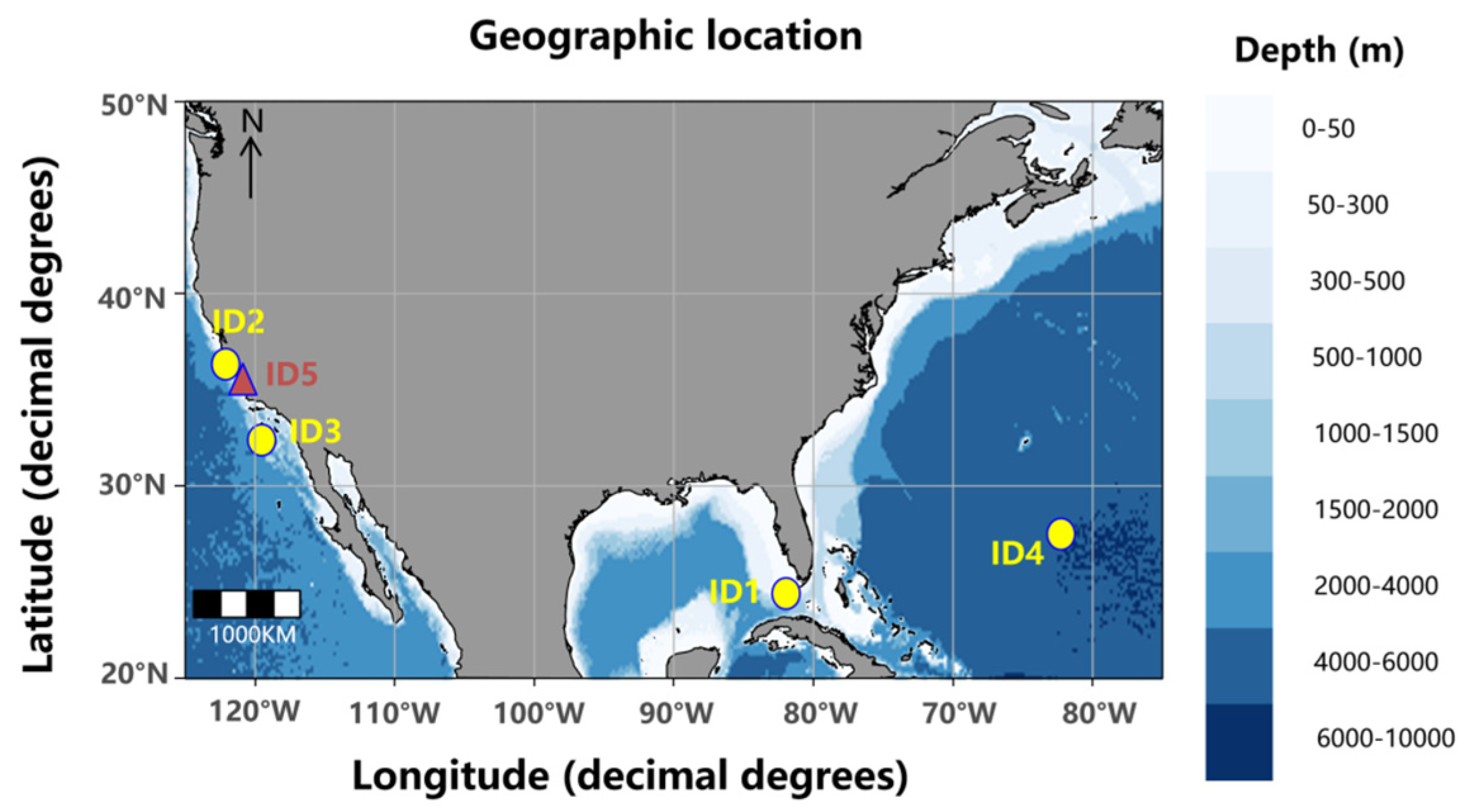
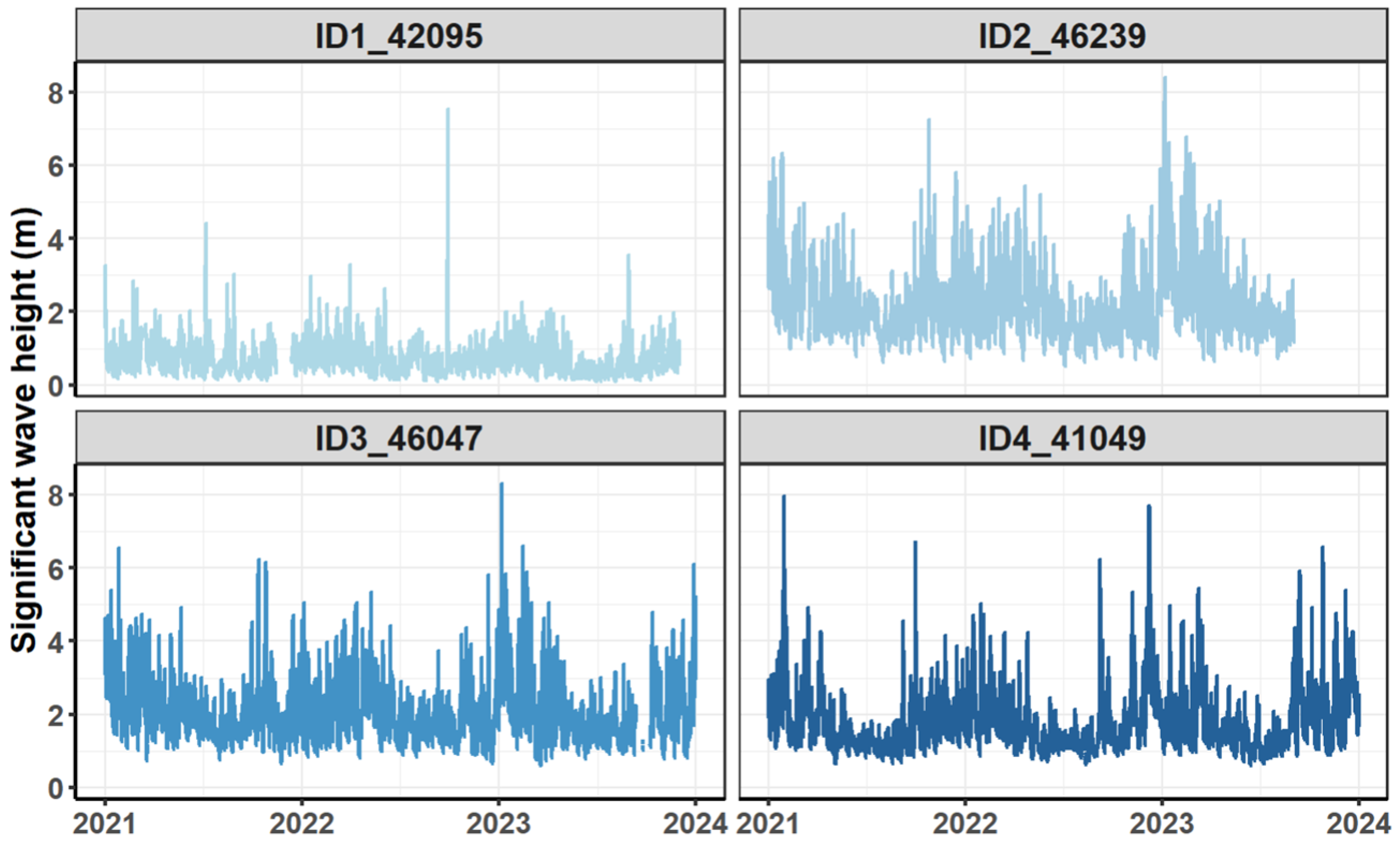
The significant wave height time series of four buoys are visualized in Figure 2. All buoys data started at 00:00 on 1 January 2021. Data for buoy ID1 are missing from 13 November 2021 at 22:00 to 12 December 2021 at 21:00. Data for buoy ID2 are missing from 2 September 2023 at 16:00 to 31 December 2023 at 23:00. The other sites also have a small portion of missing data. Nevertheless, in the case of site ID2, which had the most missing values, its raw data had 3169 missing values, which is only 12.06% of the total data.

3.2. Statistical Analysis

In this subsection, the properties of the data and the relationships among the buoys are explored from different perspectives by mutation detection, cluster analysis, density distribution, Shannon entropy calculation, and Spearman correlation test on the time series data. These analysis reveal the stability of the data series and the differences between different buoys. They also provide interpretation for the subsequent wave height prediction model from the perspective of data layer.

(1)

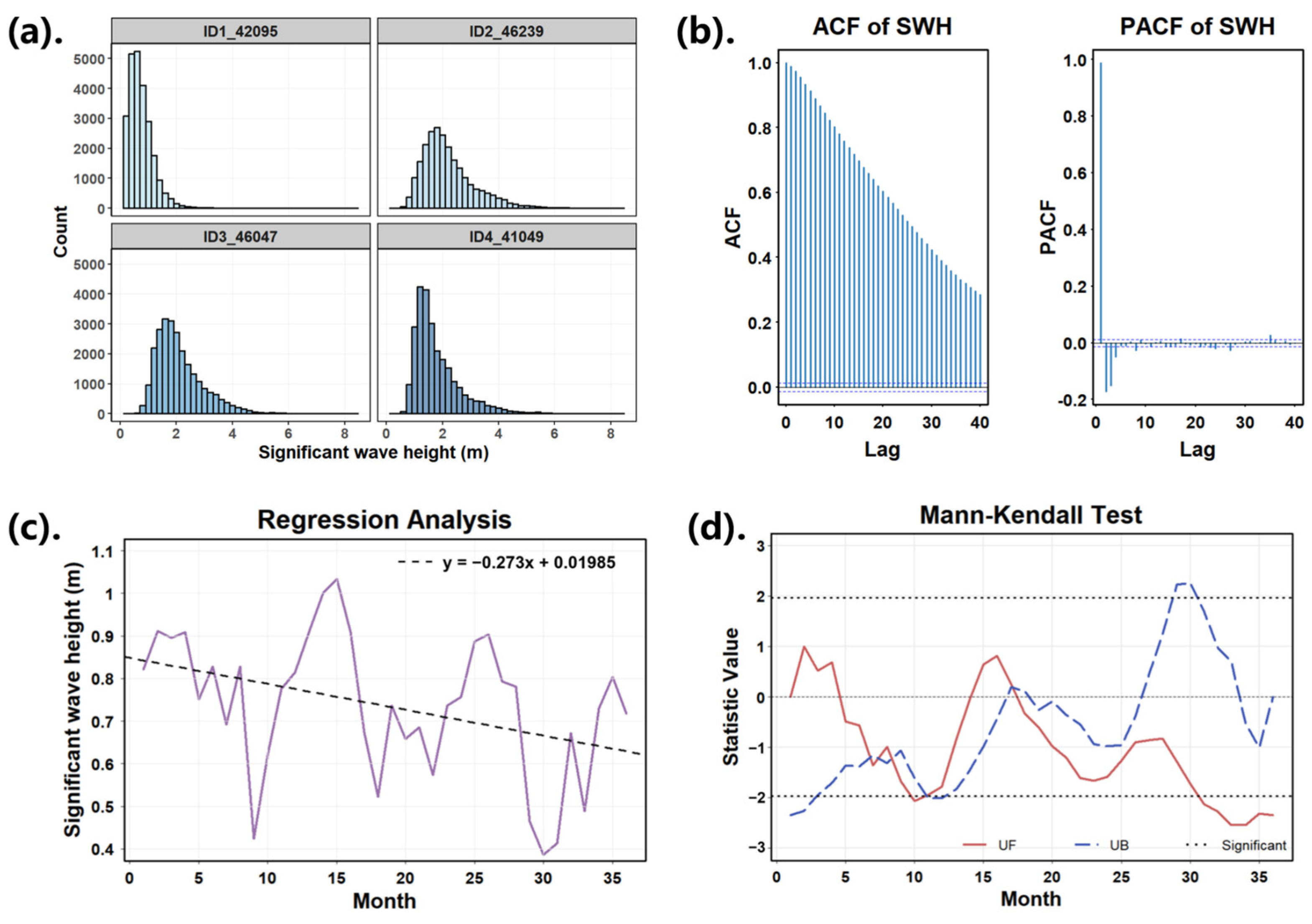
Data preprocessing and Mann–Kendall

To illustrate the analytical procedure, buoy ID1 is selected as a representative example. Autocorrelation function (ACF) and partial autocorrelation function (PACF) analysis are first performed to assess the stationarity and correlation structure of the time series (Figure 3b). Under the condition setting of the confidence level (95%), mutation detection is conducted based on the intersections of confidence intervals, and the test results are statistically validated with the t-test. Notably, the dataset contains only 36 sample points. Although a mutation point is mathematically detected at the final data point (Figure 3c,d), probably it results from boundary sensitivity of the test. The absence of significant changes throughout the observation period suggests the time series was overall stable.

(2)

Clustering analysis and visualization of density distribution

This subsection employs hierarchical clustering with incomplete linkage (hclust) based on ACF distance metrics to analyze the intrinsic similarities and differences among the buoy datasets. The clustering results demonstrate that buoy ID4 exhibits significant differences from other buoys. ID2 and ID3 show higher autocorrelation coefficients, indicating highly similar patterns in their data variations. To further validate these findings, a visual analysis of Hs density distribution is also conducted (Figure 3a). Although the majority of wave heights mainly concentrate in the range of 0 to 6 m, the distribution patterns vary noticeably between buoys. The distribution patterns of ID2 and ID3 are particularly similar.

(3)

Shannon Entropy and Quantification of Prediction

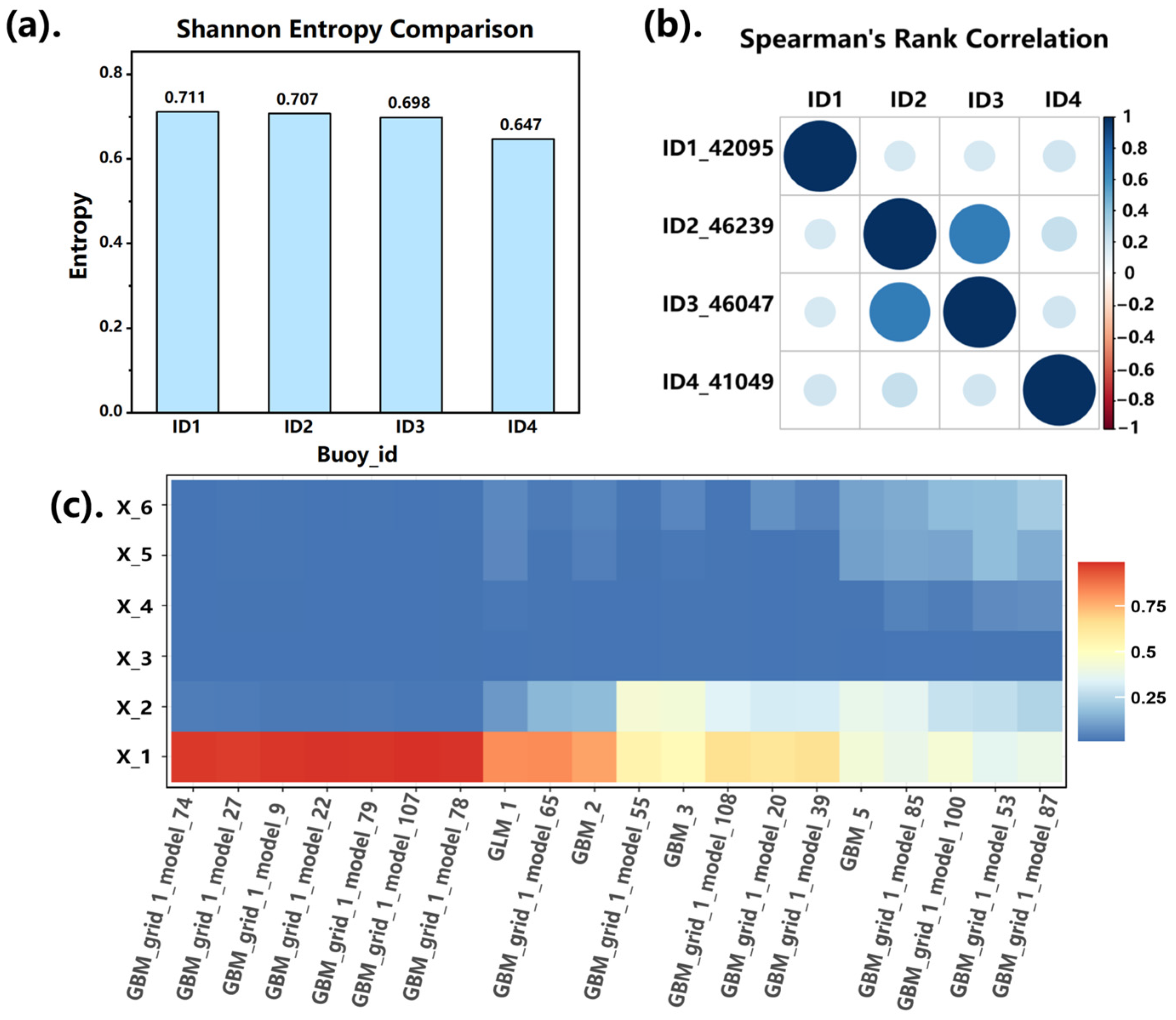
Uncertainty Shannon entropy is used to quantify the predictability of Hs time series. The experimental results (Figure 4a) show that the Shannon entropy of significant wave height for the four buoys lies between 0.647 and 0.711. This study uses entropy only as a qualitative proxy for time series complexity rather than as the subject of formal significance testing. Lower entropy (buoy ID4) implies a more regular (less complex) signal and is therefore expected to be easier to forecast, whereas higher entropy indicates richer dynamics and potentially higher forecasting difficulty.

(4)

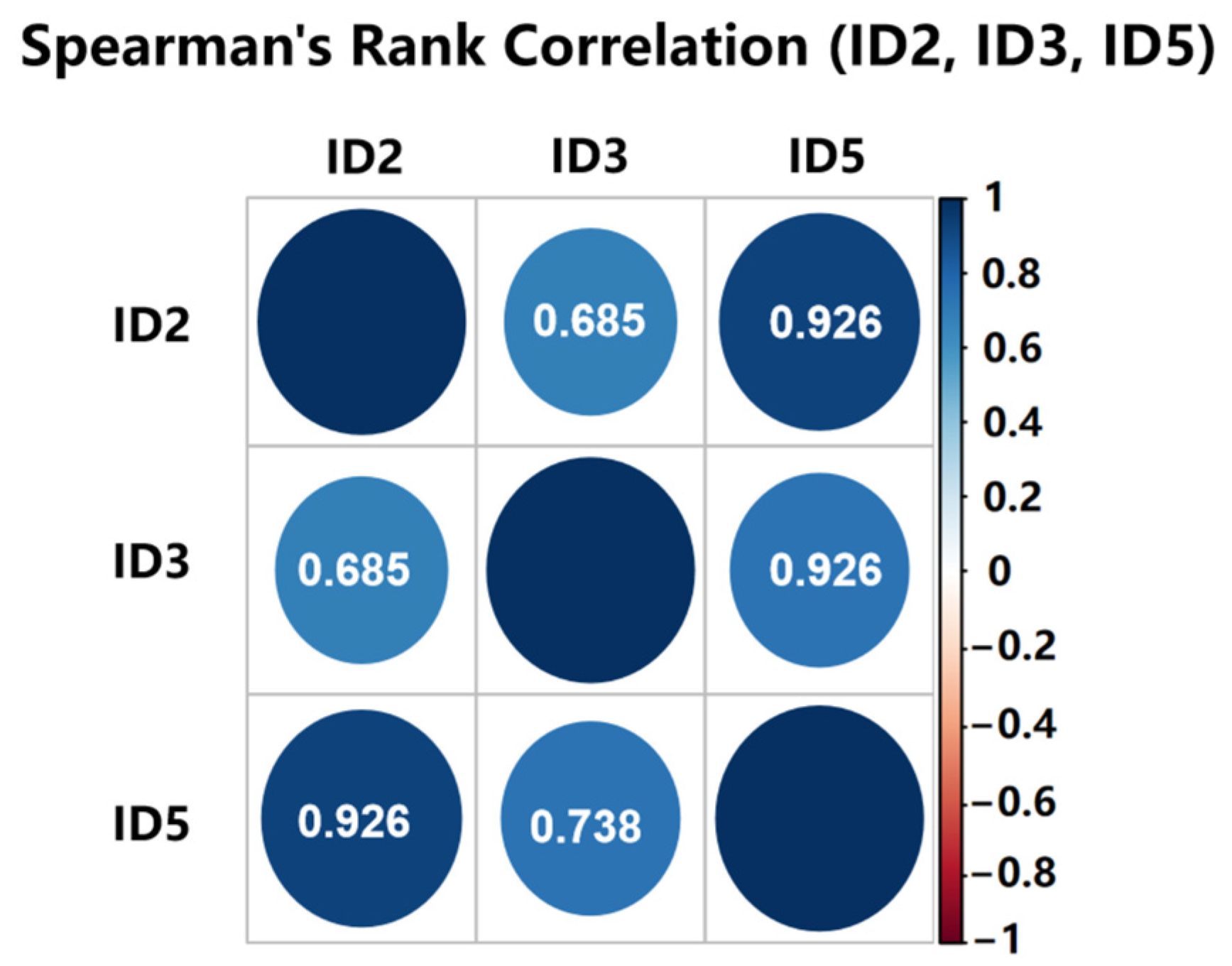
Spearman’s correlation coefficient analysis

Considering the potential non-normality of data distribution, the Spearman rank correlation coefficient is adopted to evaluate the correlation between buoys. As shown in Figure 4b, the correlation coefficient between ID2 and ID3 reaches 0.69. This number is significantly higher than that of other combinations. This result provides a theoretical basis for the subsequent data fusion strategy. It means that joint modeling using historical wave height data from neighboring stations (ID2 and ID3) could be a feasible approach for cross-station prediction.

(5)

Variable Importance Analysis

Finally, a local prediction model using a historical window length of six is constructed. Figure 4c plots the variable importance analysis and evaluates the contribution of each predictor variable to the model output. Figure 4c is a heatmap of model’s feature importance. The y-axis represents lag features (X_1 to X_6), and the x-axis shows the candidate models used during AutoML training. The color depth reflects the importance of each lag variable in each model. It shows that most models assign the highest importance to X_1 and X_2, indicating that the most recent wave heights have the strongest predictive power. Results in the figure show that the latest hour has the greatest impact on the prediction result. The darker red shading denotes higher importance. This result intuitively reflects the crucial role of closest hourly data in short-term forecasting.

In summary, the exploration analysis shows that buoys ID2 and ID3 exhibit strong correlation and similar statistical patterns, which lays a foundation for data fusion strategies. The entropy and ACF results also suggest stable, predictable time series behaviors across sites.

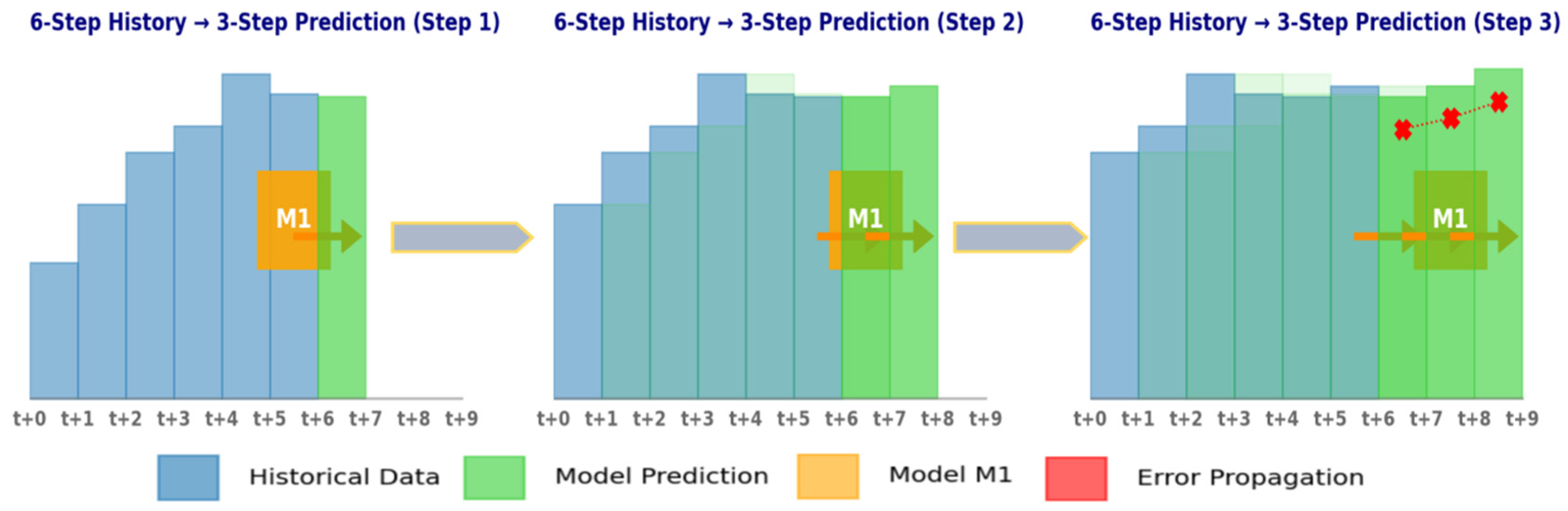
3.3. Iterative Prediction Strategy

In multi-step prediction scenarios, the model needs to obtain more feature information, especially historical sequence data. In this paper, a sliding window approach is used to create a dataset to convert time series prediction into supervised learning. At the same time, the original data are not subjected to any additional processing to retain all the original features of the data. In addition, any subsequences containing missing values within the sliding windows will be eliminated.

$${\widehat{y}}_{N+W}=\left\{\begin{array}{cc}\widehat{f}\left(y_N,y_{N-1},\dots ,y_{N-d+1}\right)\hfill & if h=1\hfill \\ \widehat{f}\left({\widehat{y}}_{N+h-1},\dots ,y_N,\dots ,y_{N-d+h}\right)\hfill & if h\in \{2,\dots ,d\}\hfill \\ \widehat{f}\left({\widehat{y}}_{N+h-1},{\widehat{y}}_{N+h-2},\dots ,{\widehat{y}}_{N+h-d}\right)\hfill & if h\in \{d+1,\dots ,W\}\hfill \end{array}\right.$$

(6)

Specifically, predicted steps refer to the quantity of future data points that need to be predicted. In multi-step prediction tasks, there are two main basic strategies: iterative prediction and direct prediction. Here, $\left[y_1,y_2,\dots ,y_N\right]$ is defined as the original input sequence, and $\left[y_{N+1},y_{N+2},\dots ,y_{N+W}\right]$ is the value of forecast ahead W steps. In the equation, d is the embedding dimension, and f is the function dependence. In particular, the core idea of the iterative strategy is to transform the multi-step prediction problem into multiple single-step prediction problems. This strategy typically involves training a model M1 that predicts values only one step ahead. During the prediction process, M1 continuously uses its previous prediction as input for the next step. The core of the direct prediction strategy lies in establishing a separate model for each prediction step. However, the model may not be able to effectively capture the temporal dependencies within the sequence and generally consume more computing resources. Therefore, this section adopts an iterative prediction strategy. Figure 5 is a schematic diagram of iterative prediction with an embedding dimension of 6, taking six historical steps to predict Hs for the next 3 h as an example.

3.4. Training Time and Lag Feature Selection

First, the H2O-AutoML algorithm is selected to construct the automatic machine learning process. Choosing the appropriate maximum search time and lag feature length for AutoML can reduce unnecessary consumption of computing resources. Three different lag feature lengths (30 steps, 45 steps, 60 steps) are selected [41], and three different search times (10 min, 20 min, 30 min) are set in all four buoy stations. The MAPE of 12 h ahead prediction is used as the evaluation metric. This is because the prediction with the longest number of steps in iterative prediction accumulates the most error and has relatively larger performance fluctuation. In the prediction of one hour, the performance differences among them are not significant (or even no difference). As a dimensionless index, MAPE is convenient for comparing performance across buoys. Moreover, the 12 h prediction accumulates the most error and can effectively reveal the performance differences in the models.

It can be seen clearly from Figure 6 that a longer search time does not necessarily mean better. A long search time may not bring significant improvement. For buoy ID1, even if the search time is extended, its MAPE value does not decrease significantly. On the contrary, for most sites, the MAPE value has reached or approached the optimal level within a 10 min search time. The MAPE values of buoys ID2 and ID3 with 10 min of search time are comparable to those with 30 min of search time. This indicates that a 10 min search duration is sufficient for the model to converge to a better solution.

Furthermore, the research finds that lag feature length significantly impacts model performance. In this experiment, 30, 45, and 60 steps are empirically chosen for comparative analysis. Among them, the 30 and 60 steps perform poorly on some sites, while the 45 step shows more stable performance on most sites. Taking buoy ID3 as an example, the MAPE value of 45 steps is lower than that of 30 and 60 steps, indicating that 45 steps can better capture the key features in the time series. While longer search time and more lag features can improve accuracy at specific sites, the 45-step/10 min configuration offers a cost-effective and stable trade-off across all the stations. It may serve as an optimized runtime setup delivering balanced performance and efficiency.

Therefore, the study chooses 10 min as the maximum search time and 45 steps as the lagged feature length. This configuration ensures optimal computational resource utilization while maintaining predictive accuracy.

3.5. Comparison of Four AutoML Frameworks

This subsection systematically evaluates the predictive performance of four AutoML frameworks (H2O, AutoGluon, PyCaret, and TPOT) in forecasting Hs across different time horizons, ranging from 1 h to 12 h. The experimental results (

Table 3. Performance of buoy ID1 in 1–12 h ahead steps under four AutoML methods.

Ahead Steps	Metrics	PyCaret	H2O	TPOT	AutoGluon
1 h	MAPE	0.075	0.075	0.866	0.079
	RMSE	0.069	0.067	0.069	0.065
	R2	0.965	0.967	0.964	0.968
3 h	MAPE	0.145	0.143	0.865	0.147
	RMSE	0.115	0.112	0.114	0.112
	R2	0.903	0.907	0.904	0.907
6 h	MAPE	0.22	0.218	0.865	0.219
	RMSE	0.166	0.163	0.166	0.164
	R2	0.797	0.802	0.799	0.808
9 h	MAPE	0.267	0.264	0.865	0.265
	RMSE	0.201	0.2	0.2	0.2
	R2	0.703	0.708	0.705	0.72
12 h	MAPE	0.302	0.299	0.864	0.299
	RMSE	0.317	0.227	0.228	0.228
	R2	0.617	0.622	0.62	0.639

,

Table 4. Performance of buoy ID2 in 1–12 h ahead steps under four AutoML methods.

Ahead Steps	Metrics	PyCaret	H2O	TPOT	AutoGluon
1 h	MAPE	0.053	0.053	0.438	0.055
	RMSE	0.157	0.158	0.16	0.158
	R2	0.961	0.961	0.959	0.96
3 h	MAPE	0.082	0.082	0.438	0.083
	RMSE	0.247	0.247	0.25	0.247
	R2	0.903	0.903	0.9	0.903
6 h	MAPE	0.119	0.119	0.439	0.119
	RMSE	0.354	0.364	0.367	0.361
	R2	0.789	0.789	0.786	0.793
9 h	MAPE	0.145	0.145	0.439	0.144
	RMSE	0.448	0.447	0.45	0.442
	R2	0.68	0.68	0.677	0.688
12 h	MAPE	0.166	0.166	0.44	0.165
	RMSE	0.51	0.511	0.513	0.505
	R2	0.584	0.583	0.58	0.594

,

Table 5. Performance of buoy ID3 in 1–12 h ahead steps under four AutoML methods.

Ahead Steps	Metrics	PyCaret	H2O	TPOT	AutoGluon
1 h	MAPE	0.052	0.058	0.421	0.057
	RMSE	0.156	0.155	0.155	0.155
	R2	0.96	0.95	0.951	0.95
3 h	MAPE	0.079	0.08	0.42	0.079
	RMSE	0.218	0.217	0.217	0.217
	R2	0.902	0.903	0.903	0.903
6 h	MAPE	0.11	0.111	0.42	0.109
	RMSE	0.308	0.307	0.306	0.305
	R2	0.805	0.807	0.807	0.808
9 h	MAPE	0.131	0.131	0.419	0.13
	RMSE	0.372	0.37	0.369	0.369
	R2	0.716	0.719	0.719	0.72
12 h	MAPE	0.148	0.149	0.419	0.148
	RMSE	0.421	0.419	0.419	0.419
	R2	0.635	0.638	0.64	0.639

and

Table 6. Performance of buoy ID4 in 1–12 h ahead steps under four AutoML methods.

Ahead Steps	Metrics	PyCaret	H2O	TPOT	AutoGluon
1 h	MAPE	0.051	0.051	0.589	0.053
	RMSE	0.145	0.144	0.148	0.152
	R2	0.977	0.977	0.976	0.975
3 h	MAPE	0.069	0.069	0.589	0.071
	RMSE	0.207	0.205	0.208	0.21
	R2	0.953	0.954	0.952	0.952
6 h	MAPE	0.096	0.096	0.588	0.097
	RMSE	0.289	0.287	0.288	0.287
	R2	0.908	0.909	0.908	0.909
9 h	MAPE	0.119	0.118	0.588	0.119
	RMSE	0.356	0.353	0.354	0.35
	R2	0.86	0.863	0.862	0.865
12 h	MAPE	0.139	0.138	0.588	0.138
	RMSE	0.412	0.408	0.408	0.403
	R2	0.813	0.816	0.816	0.821

) show that each framework improves the model selection efficiency by parallel training multiple candidate models and intelligently optimizing the combination of parameters. However, under different datasets and prediction step sizes, the performances have different emphases.

Taking the buoy ID1 dataset as an example, when the prediction horizon extends from 1 h to 12 h, H2O and PyCaret show similar short-term prediction capabilities. The 1 h predicted MAPE values from both algorithms are stable at 0.075, and the RMSE difference does not exceed 0.002. This phenomenon has also been verified on the ID2 and ID3 datasets. It implies that there may be commonalities at the algorithmic level between the two in the selection of the basic model and the setting of the parameter search space.

However, with the increase in the prediction horizon, AutoGluon gradually shows a relatively advantage. For instance, in the 12 h-ahead prediction task of buoy ID1, AutoGluon achieved an R² of 0.639, representing a 0.017 improvement over the next-best framework. This advantage becomes more pronounced on higher-quality datasets such as ID4. The result demonstrates that the framework’s ensemble strategy enhances its robustness against the degradation effects in long-term time series forecasting.

It is worth noting that the TPOT framework shows obvious metric imbalance in the experiment. Taking the data of buoy ID1 as an example, the MAPE values of each time step are abnormally high and stabilize within the range of 0.864–0.866. However, the RMSE and R-squared metrics remain at a similar level with the other frameworks. Similar trends appear in the ID2–ID4 datasets. Further analysis show that the genetic algorithm adopted by TPOT may focus excessively on the global search of the MSE in the optimization process, while there is a systematic bias in the sensitivity of the MAPE.

Meanwhile, all AutoML algorithms cannot avoid the inherent limitation that predicting performance decays with increasing step size. For instance, in the PyCaret results on buoy ID1, as the prediction time increases from 1 to 12 h, the average MAPE across frameworks increase from 0.075 to 0.302. Concurrently, R² declines from an average of 0.965 to 0.617, a decrease of about 36%. This attenuation effect varies by dataset quality: for the ID1 data with relatively large monitoring noise, the maximum R² discrepancy between frameworks at the 12 h horizon reached 0.019 (AutoGluon 0.639, TPOT 0.620). Conversely, in the higher-quality ID4 dataset (ID4 sites have the largest amount of data and the lowest missing rate), this difference narrowed to within 0.008. These results suggest that a higher signal-to-noise ratio not only improves overall predictive accuracy, but also enhances the stability and consistency of AutoML framework outputs.

The analysis above shows that these four AutoML algorithms are close in short-term Hs prediction, but in medium- and long-term prediction, the performance of each framework varies significantly. Moreover, data quality has a significant impact on the prediction. The noisy environment not only aggravates the attenuation of prediction performance, but also amplifies the impact of the differences in strategies between different frameworks. Although AutoML frameworks are similar in basic strategies, in specific applications, the final performance can differ significantly. Therefore, in practical applications, an appropriate framework should be selected based on data characteristics and predicted demands.

3.6. Model Interpretation and Assessment

Compared with AutoML frameworks such as H2O, AutoGluon, and TPOT, PyCaret demonstrates higher accuracy and faster training speed in short-term prediction tasks. These performance advantages not only enhance the overall predictive ability of the model, but also provide a solid technical foundation for model interpretation. Due to the simplification of the model construction process and the provision of rich visualization tools by PyCaret, users can understand the internal operation mechanism more easily, thereby enhancing the explainability and transparency of the model.

According to the experimental data in the previous section, PyCaret significantly outperforms the other frameworks in terms of MAPE over the 1 h–3 h time span. The stability of short-term prediction indicates its model structure is better at capturing the initial state of the time series. In view of the key role of short-term prediction in real-time decision-making of buoy monitoring, choosing PyCaret for analysis can not only effectively reveal the mechanism of action of proximal predictors, but also avoid the interference of cumulative noise on feature attribution in long-term prediction.

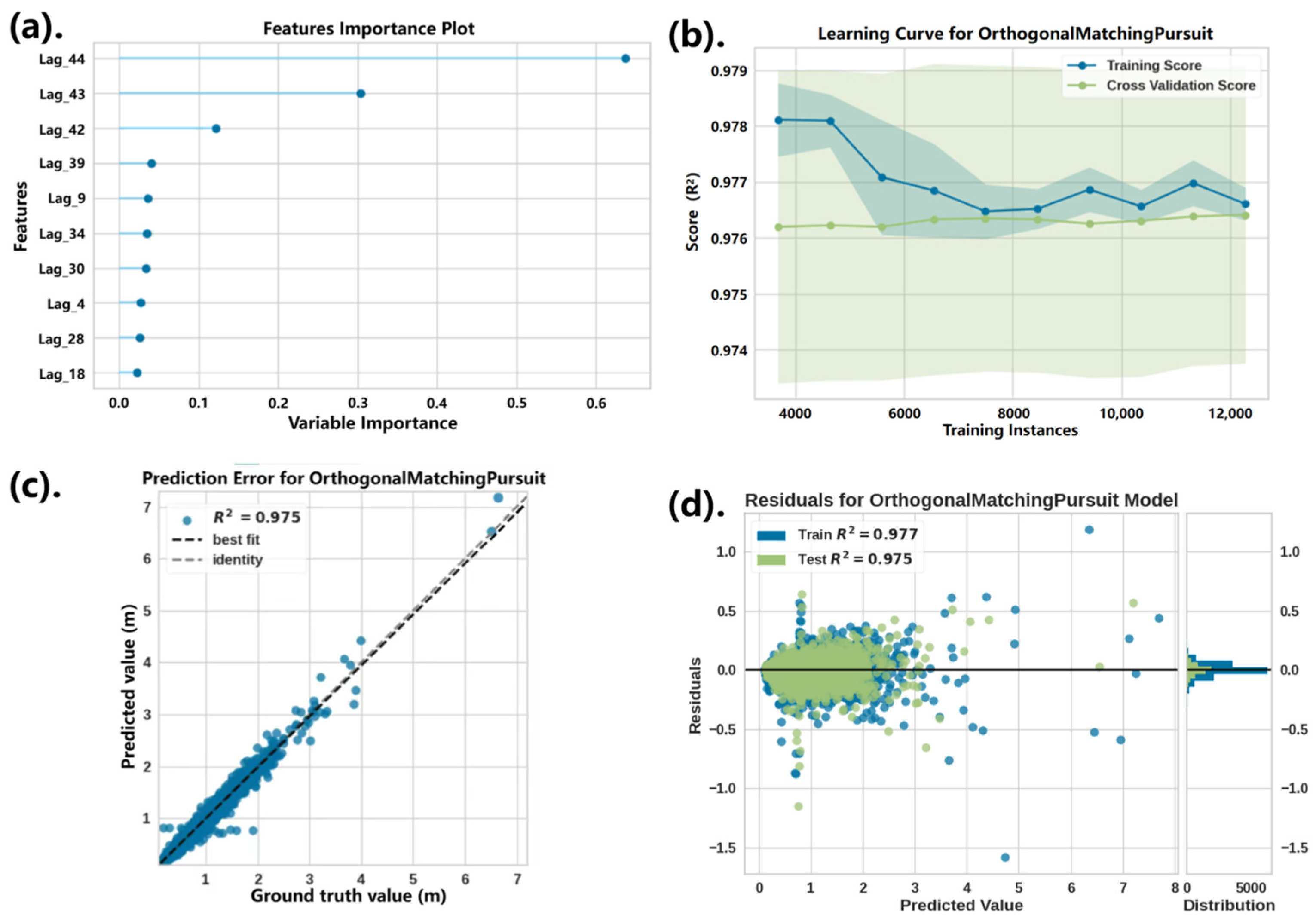
Pycaret’s compare_models() function compares multiple candidate regression models by default. The dataset used in this evaluation is the buoy ID1 data, with a lag feature length of 45 and a prediction ahead step of 1 h. The comparison after running the code shows that orthogonal matching pursuit (OMP) performs best on several metrics, outperforming other models. In the ID1 dataset, OMP has high prediction accuracy and stable generalization performance.

The sliding window length is 45, with lag features indexed from Lag_0 to Lag_44. Here, Lag_0 refers to the earliest time step in the window, i.e., the observation 45 steps before the prediction point, while Lag_44 represents the most recent observation just before the prediction. This indexing is used in Figure 7a, where feature importance is shown for each lag. As shown in Figure 7a, the characteristics of the last few hours are most important for the model’s predictions. This is consistent with general time series prediction. The closer the observation is to the current moment, the more it contributes to the next prediction. In the learning curve graph (Figure 7b), the horizontal axis represents the training sample size, the vertical axis represents the model score (R²), the dark blue curve represents the training set score, the light green curve represents the cross-validation score, and the confidence interval is indicated by the shadow. In the figure, the R² values of the training set and the cross-validation set both stabilize at around 0.975, and the gap between the two is small. The result indicates the OMP performs well in both the training and validation processes and no overfitting or underfitting occurs. The R² value of the test set is 0.975 (Figure 7d) and it is very close to the training set, which further verifies the strong generalization ability of the model.

The scatter plot of the prediction error (Figure 7c) shows the scatter distribution of the true value y versus the predicted value (ŷ). The figure presents two lines: one is the diagonal line for the ideal case, and the other is a regression line fitted based on the actual data distribution. From the figure, most of the data points are distributed near the ideal diagonal, and most of the scatter points are very close to the diagonal. It means the predicted values are highly consistent with the actual values. The scattered points deviate slightly from the diagonal at around y > 6.0 m (i.e., the part when the wave height is relatively higher). That indicates there is still some room for the model to improve its prediction of the extreme values. Overall, the residual analysis does not show obvious significant patterns, and the performance of the training set and the test set is also close. This indicates that the OMP model has good stability and consistency at the ID1 site.

Next, the comparison between the predicted and true values of PyCaret at five prediction steps is plotted (Figure 8). It can be observed from the graph that as the predicted future hour step size (1, 3, 6, 9, 12) increases, the predicted values gradually lag behind the true values. This indicates that lag effects become more pronounced in the long-term forecast. This means that the model reacts more slowly to the future trend and is unable to capture the rapid fluctuations in time.

When the prediction step is short, the prediction curve closely aligns with true values and accurately tracks fluctuation trends. In contrast, as the prediction step size increases, the model error gradually accumulates, resulting in a larger overall deviation of the prediction curve. This is because the model can make predictions based on relatively accurate historical data in a short period of time. However, errors will accumulate continuously when the prediction step size increases. It will lead to a decrease in the medium-term and long-term prediction reliability.

4. Multi-Point Data Fusion Prediction

The performance of four mainstream AutoML frameworks in single-point Hs prediction has been systematically evaluated, revealing their strengths and weaknesses across varying prediction horizons. Results show that although AutoGluon exhibits stronger antidecay capability in medium-term and long-term predictions, and the accuracy of all frameworks remains highly dependent on the amount of historical data available at the target site. Specifically, when the target site lacks sufficient local historical observations, model performance may deteriorate, exposing the constraints of single-point prediction approaches in data-scarce scenarios.

Based on these findings, a cross-station prediction framework incorporating multi-point data fusion is proposed. The approach integrates Hs time series features from geographically adjacent stations (buoys ID2 and ID3) with Principal Component Analysis (PCA) and feature space reconstruction techniques. The framework captures shared feature patterns across multi-source data within a single training process, enabling effective prediction at unmonitored locations (buoy ID5). This method seeks to mitigate model overfitting under sparse data conditions, while offering a more generalizable and scalable solution for multi-station collaborative monitoring and broad-area prediction in practical marine environments.

It should be noted that the study confines the application of the multi-point data fusion framework to a specific sea area. The station used as the target (ID5) and the stations used as data bases (ID2 and ID3) are all located on the California coast. Hs at the three stations are found to be quite relevant, and they belong to an area that basically shares the same meteorological mechanism.

4.1. Experimental Data

Three buoy stations (ID2, ID3, and ID5) are selected based on their significant spatial correlations. The variable correlations between the sites are quantitatively reflected by Spearman’s rank correlation coefficient (ρ) matrix analysis. Results reveal a strong positive correlation between buoys ID2 and ID5 (ρ = 0.926, p < 0.001), while buoy ID3 is also highly correlated with ID5 (ρ = 0.738, p < 0.001). This differentiated correlation pattern may be attributed to spatial distribution characteristics. Buoy ID5 has minimal longitudinal separation (0.2°) and moderate latitudinal distance (0.57°) from ID2, while its latitudinal difference with ID3 spans 3.35°. The closer spatial distance may lead to more significant coupling effects of environmental parameters. The results of the correlation matrix (Figure 9) further confirm this finding.

This study adopts the non-parametric Spearman’s correlation coefficient. This selection is mainly due to the non-normality characteristics of data distribution and the existence of outliers [42]. The method exhibits superior robustness to variations in data distribution patterns.

4.2. Methods

A time series wave height prediction framework based on multi-source buoy data fusion is proposed. The core workflow of this framework includes data standardization, feature-level fusion, spatiotemporal feature reconstruction, and automated machine learning modeling. The framework introduces Principal Component Analysis (PCA) to realize the feature space alignment of heterogeneous sensor data. This is combined with a sliding window mechanism to capture nonlinear temporal dependencies of wave height. Given the magnitude difference and potential sensor drift in the raw wave height data from buoy ID2 and buoy ID3, these datasets are normalized with

$$z={\displaystyle \frac{x-\mu }{\sigma }}$$

(7)

where μ denotes the sample mean and σ represents the standard deviation. The StandardScaler function is applied to standardize the significant wave height data, transforming it to have zero mean and unit variance. For the non-stationary characteristics of marine environmental data, an independent normalization strategy for each buoy is adopted to avoid the normalization distortion caused from cross-station distributional differences.

To effectively extract the common fluctuation patterns of multi-source data, a feature fusion module based on Principal Component Analysis (PCA) has been designed. The normalized ID2 and ID3 wave height data are used to form the feature matrix $X\in R^{n\times 2}$, and the optimal projection direction is solved by singular value decomposition (SVD). The projection matrix is constructed by taking the largest eigenvalue corresponding to the eigenvector v₁, thereby reducing the original two-dimensional feature space to a one-dimensional fused feature representation.

$$X^{T}X=V\Sigma V^T, z=X{v}_1$$

(8)

This process preserves as much of the covariance information from the original data as possible, and suppresses cumulative sensor noise effects. Experimental results confirm that the first principal component (PC1) cumulatively could explain 86.7% of the variance (Figure 10a,b). Given this, PC1 captures the majority of the data’s essential information and can be the primary feature for dimensionality reduction. The boxplot in Figure 10c shows the distribution of PC1 in different months. While the median remains relatively stable across months, variance increases significantly during winter, which may indicate that the sea state is more unstable in winter.

The scatterplot (Figure 10d) distinguishes data points with colors from different locations using PC1 and PC2 as axes, respectively. The data from both sites are distributed along a certain main direction, further indicating their Hs data patterns are similar. Since most data points cluster in a single directional trend, this pattern indicates that both stations share similar primary variation trends. These findings demonstrate PCA’s effectiveness in extracting common features.

Based on the temporal and spatial continuity characteristics of wave propagation, a sliding window mechanism is constructed to extract the time series dependent features. A timestamp intersection strategy was used to align ID2 and ID3, retaining only the time steps where both buoys have available data to ensure temporal synchronization. Given the history window length T = 45 and the prediction horizon τ = 1, the sample reconstruction function is defined as

$$F:{\mathrm{z}}_{\mathrm{t}-\mathrm{T}+1},\dots ,{\mathrm{z}}_{\mathrm{t}}\mapsto {\mathrm{z}}_{\mathrm{t}+\mathsf{\tau }}$$

(9)

A set of supervised learning samples is generated through a rolling time window. Each sample consists of the fused feature values from 45 consecutive time steps, and the output is Hs observation at the next instant. This strategy transforms the time series prediction problem into a supervised learning task.

4.3. Performance Evaluation of Prediction Models

This subsection employs the AutoGluon framework to develop a multi-step forecasting model for Hs of Buoy ID5 (46028). AutoGluon is chosen because it shows robust advantages in some scenarios. During Section 3 for buoys ID3 and ID2, AutoGluon achieves the lowest MAPE and a high R-square, showing its stability and adaptability in parameter optimization. By comparing the forecasted values with the observed data, the system evaluated the prediction performance of the model in the time range of 1 h to 24 h. This subsection quantitatively assesses the model’s capability in Hs forecasting. The evaluation particularly focuses on temporal scalability from single-step (1 h horizon) to multi-step predictions (3 h, 6 h, 12 h, and 24 h horizons).

As shown in

Table 7. Results of the metrics.

Metric	1 h	3 h	6 h	9 h	12 h	24 h
MSE	0.031	0.090	0.174	0.259	0.345	0.770
$R^2$	0.976	0.929	0.862	0.795	0.725	0.382
MAE	0.129	0.215	0.298	0.360	0.421	0.629

, the model exhibits excellent performance in single-step prediction (1 h), achieving an MSE of 0.031, R² = 0.976, and MAE = 0.129. These metrics suggest that the model can accurately capture the short-term dynamics of the wave parameters. However, all the metrics show obvious degradation when the prediction horizon extends to 24 h. Within the 1 h, 3 h, and 6 h ranges, the correlation between the predicted and observed values remains high. Nevertheless, error accumulation becomes increasingly significant with longer forecast lead times, manifested by a substantial increase in MAE from 0.129 (1 h) to 0.629 (24 h).

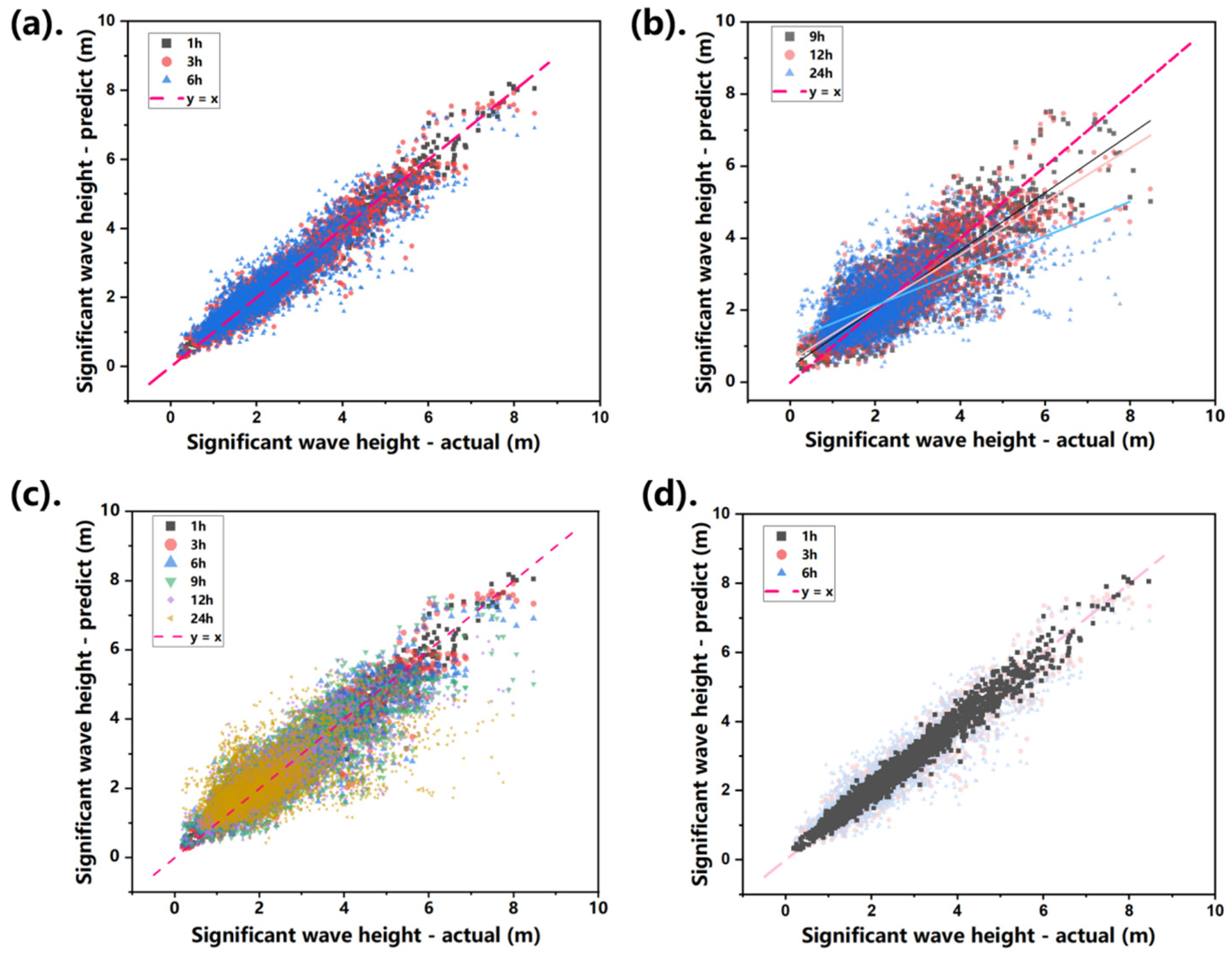
Figure 11 is helpful for qualitatively comparing prediction performance. Figure 11a presents the scattered distribution of the predicted and actual values of Hs under short-term predictions (1 h, 3 h, and 6 h), distinguished by marker label and color. Among them, Figure 11d shows the 1 h prediction (black squares) from Figure 11a in detail. Most of the data points are distributed in the area close to y = x. Figure 11b similarly presents results for medium- and long-term predictions. For a consolidated view, Figure 11c combines all six horizons on one graph, where scatter dispersion visibly increases with forecast horizons.

5. Conclusions

Short-term Hs prediction is critical to marine operation decision-making (e.g., window selection) and ship route optimization. This study evaluated four mainstream AutoML frameworks (H2O, PyCaret, AutoGluon, and TPOT) on their prediction performance and the reasons for differentiation. For short-term predictions, PyCaret demonstrates superior accuracy due to its model stability and interpretability. The PyCaret OMP model excels in feature capture and generalization capabilities and is suitable for real-time monitoring scenarios that require rapid decision-making. With the extension of the prediction time span to medium-term and long-term, AutoGluon shows a stronger anti-attenuation capability. AutoGluon can effectively suppress the cumulative effect of errors (through ensemble strategies and parameter optimization mechanisms) and has become the preferred tool for complex time series modeling.

Notably, the TPOT framework exhibits significantly higher MAPE than other frameworks, attributed to the genetic algorithm’s inherent insensitivity to percentage error metrics. Although TPOT achieves comparable RMSE and R² scores to other methods, this limitation restricts its applicability in scenarios with high-precision requirement. Datasets with greater noise intensify the accumulation of errors in long-term predictions and the differences between frameworks, while data with a high signal-to-noise ratio significantly enhance the robustness of each framework and narrow the performance gap. Overall, the appropriate framework needs to be chosen according to the specific needs in practical applications. PyCaret is recommended for short-term high-precision prediction, while AutoGluon is preferred for medium-term and long-term complex tasks. Furthermore, improving data quality should be emphasized to maximize model performance.

Additionally, a multi-station data fusion strategy is proposed as a potential solution for improving spatial generalization. By integrating time series data from two adjacent buoy stations and combining Principal Component Analysis (PCA) with AutoML, a cross-station prediction framework is constructed. The results demonstrate that the model integrating multi-site data performs well at adjacent (high-relevance) stations not directly involved in the training process. This finding implies that capturing common fluctuation patterns from multi-source data could be a promising approach for alleviating the spatiotemporal limitations of single-point datasets. The data fusion strategy could reduce reliance on single-station data, and thereby lessen the potential risks caused by sensor failures or data omissions.

In the future, a dynamic weighting mechanism can be introduced, and the satellite remote sensing and meteorological reanalysis data can also be utilized to improve the accuracy of cross-station prediction. In view of the problems such as the lack of automatic processing of data and the reliance on manual feature engineering, a more intelligent end-to-end AutoML framework will be developed in future studies.