A Deep Learning Framework for Parameter Estimation in 1D Marine Ecosystem Model

Abstract

Marine ecosystems play an increasingly critical role in both global climate regulation and the impacts of anthropogenic activities. Accurate marine biogeochemical numerical models are essential tools for understanding and predicting the complex dynamics of these systems. However, as model complexity increases, so does the number of biological parameters and the uncertainties associated with them, which can substantially affect model performance. Consequently, efficient and reliable parameter estimation has become a key challenge in model development and application. In this study, we proposed a deep learning-based approach for parameter estimation in numerical models, utilizing deep neural networks to capture the complex nonlinear relationships between numerical model input parameters and output variables. A one-dimensional marine ecosystem model is employed as a case study to evaluate the effectiveness of the proposed method. The results demonstrate that (1) the deep learning approach provides an automated and adaptive solution for parameter estimation, significantly improving the efficiency of model calibration in engineering and scientific applications by enabling rapid identification of near-optimal parameter sets; and (2) the deep learning model effectively learns the underlying nonlinear mappings between inputs and outputs. During training, the mean squared error (MSE) loss exhibits a steady decline, with minor fluctuations in the early stages, ultimately converging to a stable value. The predicted parameter combinations show strong agreement with the reference numerical model outputs, yielding correlation coefficients exceeding 0.95.

1. Introduction

Marine ecosystems are among the most complex ecosystems on Earth, playing a vital role in global climate regulation and supporting human activities [1]. Marine ecosystems are known for their rich biodiversity and are highly sensitive to environmental change and anthropogenic activities [2]. Thus, a comprehensive understanding and accurate prediction of changes within marine ecosystems are essential not only for ecological conservation but also for developing sustainable management strategies, maintaining ecological balance, and ensuring the sustainable use of resources.

In recent years, marine ecosystem dynamics modeling has emerged as a powerful tool for investigating marine ecosystems and forecasting their changes [3,4,5]. Riley et al. [6] introduced inter-population competition and predation relationships into numerical models, used phytoplankton as a state variable, and established a set of one-dimensional marine ecological dynamics models applied to the European North Sea for the first time, which quantitatively analyzed the ecological processes of phytoplankton, and became a milestone in the development of marine ecological models. With the improvement of computational conditions, the ecological model has developed greatly, the state variables considered have gradually increased, the temporal resolution has been significantly improved, and models such as two-component (NP), three-component (NPZ), and four-component (NPZD) have appeared successively [7,8,9]. The simple NPZD model lacks sufficient ecological variables for broader application. To better understand and simulate complex ecosystems, additional variables must be incorporated. When considering nutrients in the model, researchers have introduced limitations of elements such as iron and silicon beyond nitrogen and phosphorus. For plankton growth, phytoplankton are classified by size, and zooplankton are grouped into different categories based on body size, incorporating various feeding strategies and interspecies competition. Some models now include higher trophic levels, such as fish, and benthic organisms, further improving ecosystem simulations. Models are becoming more sophisticated in their simulation of ecosystems and more comprehensive in their coverage of food web relationships in marine biogeochemical cycles.

Allen et al. [10] combined the European Regional Seas Ecosystem Model (ERSEM) with a turbulence model to reproduce biomass and primary productivity in the European North Sea. The ERSEM model classified zooplankton and plants into different categories according to cell size and body size, respectively, and took into account the metabolic processes of benthic organisms, simulating the overall structure of the ecosystem and providing new insights into the interactions between different organisms and the cycling of materials. Fennel et al. [11] successfully developed a whole food web numerical model, including a fish production model and a biogeochemical model, in the Baltic Sea, where the food chain structure is relatively simple. It revealed important applications of marine ecological modeling to fishery resources. Based on the NPZD ecosystem model, Chai et al. [12] developed a more comprehensive and complex ecological model—the Carbon Silicate Nitrate Ecosystem (CoSiNE)—with ten components to investigate nitrogen and silicate cycling in the equatorial Pacific. This model incorporates iron limitation in the growth rate parameters of diatoms. It is capable of reproducing the nutrient structure, growth, and metabolic processes of plankton in equatorial waters, and has been widely cited in subsequent studies. With the continuous development of the CoSiNE ecosystem model, it has been widely applied to various scientific studies, such as mesoscale eddies [13], Kuroshio intrusion fronts [14], particulate organic carbon export [15], ecological impacts of cross-shelf exchange [4,5], ocean hypoxia [16], and upwelling ecosystems [17]. These studies have applied and validated the CoSiNE ecosystem model, demonstrating its capability to effectively represent key marine ecological processes. Details of the ecological model can be found in previous studies [3,12,13,15]. Overall, the models have evolved from simplified equations in the early days to now being able to cover a wider range of components. This series of advances has led to better numerical ecological modeling that can be applied to a wider range of marine areas and in different research directions.

Numerical ecological models require appropriate parameters to obtain better simulation results. Therefore, the optimization of marine ecological model parameters is particularly important. Previous studies have extensively explored parameter optimization for ecological numerical modeling. Initially, researchers generally used field sampling and experimental methods to obtain a portion of the ecological parameters in the model, and then used the results of the model simulations to test the reasonableness of the ecological parameter values in turn. However, a significant proportion of parameters in numerical models are not directly measurable by observational means [18], and can only be determined by reference to previous studies or model experience in other areas [19], and some model parameters can only be estimated and tested repeatedly to determine reasonable values.

From a mathematical point of view, parameter optimization of numerical models can also be interpreted as a best value problem. Many studies have used observational data for data assimilation to minimize the discrepancy between numerical marine ecological models and actual observations to invert the parameters of the numerical models. Common methods used for parameter optimization in these models include function fitting, stepwise revision, optimal interpolation, Kalman filter, heuristic search method, and variational techniques (both 3D and 4D variational methods) [20,21,22,23,24]. Doron et al. [25] used the Kalman filter to estimate the parameters of a three-dimensional ecological model of the North Atlantic Ocean, and found that the phytoplankton biomass of the model was very sensitive to parameter variations and had strong nonlinear characteristics, and that the Kalman filter method could optimize most of the ecological parameters of the model and reduce the model error. Additionally, Monte Carlo global stochastic search methods, such as simulated annealing and genetic algorithms, are frequently utilized. Hoshiba et al. [26] used genetic algorithms to optimize 23 ecological parameters to improve the model’s simulation of seasonal changes in phytoplankton biomass and accurately reveal the timing of algal bloom events.

Although a large number of optimization algorithms have been proposed in previous studies, all of them are able to optimize the parameters to some extent and improve the accuracy of the model simulation. However, due to the complexity of the ecological numerical modeling process and the interdependence of the parameters in the model [27], these optimization methods have difficulty solving the multi-parameter nonlinearity problems and are prone to local minima. Therefore, a parameter optimization method that enables more efficient parameter acquisition and avoids local optima is urgently needed to address the challenges of parameter interdependence and nonlinear problems in ecological numerical simulations.

The rapid advancement of artificial intelligence (AI) technology may offer a promising alternative solution to this challenge. AI can “learn” the features and correlations between inputs and outputs through supervised training on large datasets [28,29]. This capability makes AI particularly well-suited for problems where causal relationships between inputs and outputs are known, but the establishment of an accurate analytical physical model is too complex [30]. By leveraging AI, researchers can potentially build simplified models that effectively capture the relationships between variables and parameters in marine ecological numerical models. Therefore, this study aims to develop a deep learning-based parameter estimation method for ecological numerical models. We hope this statistical optimization model will effectively learn the nonlinear relationships between the parameters and the variables within the numerical model. The structure of this paper is as follows: Section 2 details the experimental procedures, including the configuration of the one-dimensional numerical model and the setup of the deep learning (DL) model. Section 3 presents the primary experimental results. In Section 4, the advantages and limitations of the research methods are analyzed and compared. Finally, Section 5 summarizes the findings of this study.

2. Methods

In this study, we proposed a deep learning-based approach for estimating the parameters of the marine ecosystem model (ME). The implementation of the method is based on a one-dimensional numerical model, which is combined with neural network technology to automate the parameter estimation process. First, we outline the experimental setup. Next, we present the basic structure and assumptions of the one-dimensional numerical model, discussing its role in simulating marine ecological processes. We then introduce the key parameters of the ME model that need to be estimated, providing an overview of their role in the model. Following this, we present the deep learning framework employed in this study, including the design of the neural network architecture, the structure of the input and output data, the training process, and the computational configuration.

2.1. Experiment Setup

The purpose of this study is to use DL methods to construct a link between variables (

Table 1. List of CoSiNE-13 model variables.

Name of State Variables	Symbol	Tracer Number	Unit
Nitrate	NO3	1	mmol/m3
Silicate	SiO4	2	mmol/m3
Ammonium	NH4	3	mmol/m3
Small Phytoplankton	S1	4	mmol/m3
Diatom	S2	5	mmol/m3
Microzooplankton	Z1	6	mmol/m3
Mesozooplankton	Z2	7	mmol/m3
Detritus Nitrogen	DN	8	mmol/m3
Detritus Silicon	DSi	9	mmol/m3
Phosphate	PO4	10	mmol/m3
Dissolved Oxygen	DOX	11	mmol/m3
Dioxide Carbon	CO2	12	mmol/m3
Alkalinity	ALK	13	meq/m−3 mmol/m3

) and parameters (

Table 2. List of CoSiNE parameters.

Descriptions	Symbols	Values Threshold	Descriptions
Phytoplankton	gmaxs1	2.0–4.0	Maximum growth rate for S1
	gmaxs2	2.0–4.0	Maximum growth rate for S2
	pis1	0.5–2.0	Ammonium inhibition factor for S1
	pis2	0.1–2.0	Ammonium inhibition factor for S2
	kno3s1	0.1–2.0	half-saturation constants of NO3
	knh4s1	0.1–2.0	half-saturation constants of NH4
	kpo4s1	0.1–2.0	half-saturation constants of PO4
	kno3s2	0.1–2.0	half-saturation constants of NO3
	knh4s2	0.1–2.0	half-saturation constants of NH4
	kpo4s2	0.1–2.0	half-saturation constants of PO4
	ksio4s2	0.1–2.0	half-saturation constants of SiO4
	ak1	0.0–1.0	background light extinction
	ak2	0.0–1.0	light extinction coefficient for phytoplankton
	gammas1	0.0–1.0	Mortality rates for S1
	gammas2	0.0–1.0	Mortality rates for S2
Zooplankton	beta1	0.0–1.0	Maximum grazing rates for Z1
	beta2	0.0–1.0	Maximum grazing rates for Z2
	gamma1	0.0–1.0	the assimilation rates for Z1
	gamma2	0.0–1.0	the assimilation rates for Z2
	gammaz	0.0–0.1	Mortality rate for Z1 and Z2
	kex1	0.0–0.5	They are the excretion rates for Z1
	kex2	0.0–0.5	They are the excretion rates for Z2
Others	wss2	0.0–10.0	Settling velocities S1
	wsdn	0.0–20.0	Settling velocities DN
	wsdsi	0.0–40.0	Settling velocities DSi

) in numerical models. We hope to obtain effective parameter combinations by inputting variable data into the DL model. The datasets used in the study are all derived from one-dimensional numerical model experiments. Our approach consists of two main phases (Figure 1). In step 1, the ME numerical model we established contains approximately 40 ecological parameters. We select the 25 key parameters (Table 2) and within the defined threshold values of these parameters, randomly generate 50 parameter sets (50, 25). These parameters of ME model combinations are input into the ME model to obtain the corresponding time series of 50 output variables (50, 13, 60, 1095), where 50 represents 50 sets, 13 represents 13 variables, 60 represents 60 layers for each variable, and 1095 represents 1095 days. We used ME-model variables as inputs to the DL model and ME model parameters as labels for DL model training. In step 2, after obtaining the optimized DL model, we use the ME model variable data from the testing dataset as the DL model’s input to generate parameters. Since numerical models may yield identical results under different parameter combinations [31,32], we input the parameter combinations generated by the AI model into the numerical model to regenerate multiple sets of variables (RVar), thereby evaluating the performance of the AI-derived parameter combinations in practical applications. Finally, we assess the performance of the DL model by comparing the differences between the RVar dataset and the ME model variable dataset using a series of performance metrics.

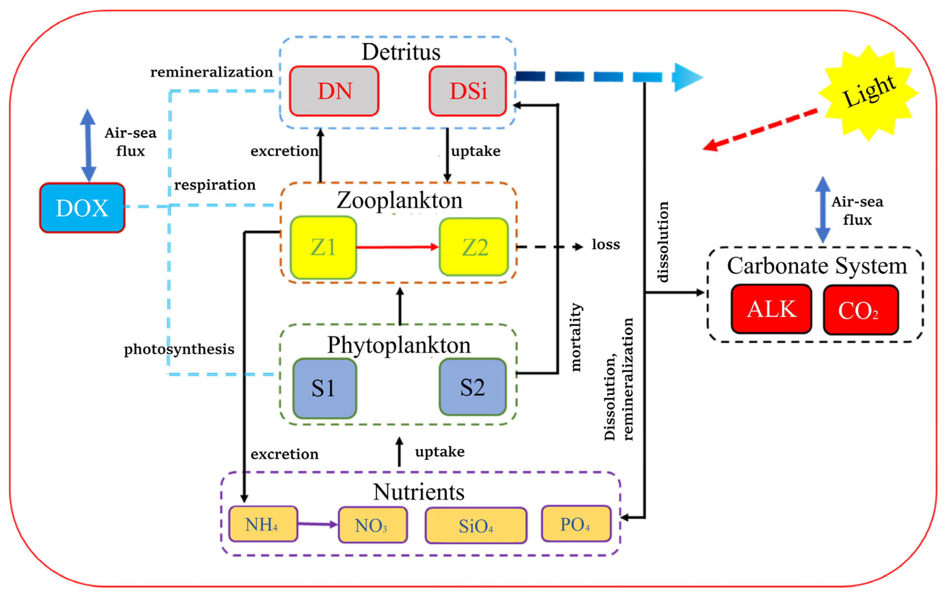
2.2. One-Dimensional Numerical Model

In this study, a one-dimensional biogeochemical coupled model was established near the Pearl River Estuary (21.472554° N, 113.875° E) to simulate the variation in nutrients in the northern South China Sea. Compared to three-dimensional models, the one-dimensional model simplifies physical processes, reduces overall model complexity, and highlights the nonlinear relationships in ecological processes, thereby facilitating the estimation and comparison of ecological parameters. Since the modeling area is far from riverine influences, and vertical diffusion is the key process for nutrient vertical transport, we simplified the physical processes of the model by including only the vertical diffusion term. The vertical domain is discretized into 60 layers, with enhanced resolution near the surface to better capture upper-ocean mixing processes. Vertical diffusion is represented by a one-dimensional diffusion equation and is implemented using a finite-difference numerical scheme.

The marine ecosystem module selected for this study is the CoSiNE-13 model (Figure 2), which was originally developed by Chai et al. for modeling the ocean biogeochemical processes for the equatorial Pacific and the Pacific Ocean [12]. The initial conditions employed in this study to establish the one-dimensional coupled physical–biological model were derived from the outputs of the Regional Ocean Modeling System–Carbon, Silicate, and Nitrogen Ecosystem (ROMS–CoSiNE) model developed by Fang et al. [4]. Atmospheric forcing fields, including air temperature, relative humidity, wind speed, sea level pressure, total cloud cover, and net shortwave and longwave radiation, were obtained from the fifth-generation European Centre for Medium-Range Weather Forecasts (ECMWF) reanalysis (ERA5) dataset. All ecological processes and formulations follow the standard definitions outlined in the CoSiNE technical manual [33]. In the CoSiNE-13 model, there are 13 state variables, including 2 phytoplankton species (S1 and S2), 2 zooplankton species (Z1 and Z2), 3 nitrogen forms (NO₃, NH₄, and DN (detritus nitrogen)), 2 silicon forms (SiO4 and DSi (detritus silicon)) and 1 phosphorus form (PO₄), dissolved Oxygen (DOX), total carbon dioxide (CO₂), and total alkalinity (ALK). The symbol and numbering in the CoSiNE-13 model for each variable are listed in Table 1 and the corresponding mathematical formulas for these variables are provided in Appendix A. The CoSiNE model code used in this study has been publicly released on GitHub (Version:CoSiNE-13; Available online: https://github.com/schism-dev/schism/tree/master/src/COSINE; accessed on 5 June 2024), accompanied by comprehensive documentation detailing model configuration, input data formats, and execution procedures. This ensures that the simulation process described in the manuscript can be fully reproduced by readers.

This research optimized key parameters in the CoSiNE-13 model, with all parameter ranges set based on previous studies [3,12,13,15,18,34,35]. For the sake of clarity and management, these parameters were categorized into the following 3 main groups: phytoplankton-related parameters, zooplankton-related parameters, and other parameters. The key parameters within each group are introduced as follows:

(1)

Phytoplankton-related Parameters

These parameters govern the growth, reproduction, and mortality rates of phytoplankton, as well as their interactions with environmental factors such as light, temperature, and nutrient availability. Key parameters include the Maximum Growth Rate (gmaxs1, gmaxs2), which determines the maximum rate at which phytoplankton S1 and S2 can grow under optimal conditions, directly influencing the overall productivity of the phytoplankton populations. The Ammonium Inhibition Factor (pis1, pis2) represents the inhibitory effect of ammonium on the growth of phytoplankton S1 and S2, helping model the negative impact of elevated ammonium concentrations on phytoplankton productivity. The Half-Saturation Constants for Nutrients (kno3s1, knh4s1, kpo4s1, kno3s2, knh4s2, kpo4s2, ksio4s2) represent the half-saturation constants for various limiting nutrients (e.g., nitrate, ammonium, phosphate, carbon dioxide, and silicate) and determine the concentration at which phytoplankton growth is half of the maximum rate, influencing nutrient uptake and overall growth. The Light Extinction Parameters (ak1, ak2) are used to calculate light attenuation in the water column, governing how light is absorbed and scattered in the water, thus influencing the availability of light for phytoplankton photosynthesis. The Mortality Rate (gammas1, gammas2) describes the natural mortality rates of phytoplankton S1 and S2, modeling the death of phytoplankton due to factors such as predation, disease, or environmental stress.

(2)

Zooplankton-related Parameters

These parameters regulate the dynamics of zooplankton populations, including their feeding behavior, growth, mortality, and the interaction between zooplankton and phytoplankton. Key parameters include the Maximum Grazing Rate (beta1, beta2), which defines the maximum rate at which zooplankton species Z1 and Z2 graze on phytoplankton, directly influencing the zooplankton population’s growth rate. Assimilation rates (gamma1, gamma2) control the efficiency with which zooplankton convert consumed phytoplankton biomass into their own biomass, with gamma1 for microzooplankton Z1 and gamma2 for mesozooplankton Z2. The Mortality Rate (gammaz) determines the mortality rate of zooplankton due to predation, disease, or environmental stress, directly impacting their population dynamics. The Excretion Rates (kex1, kex2) govern the excretion rates of zooplankton species Z1 and Z2, influencing nutrient cycling and the availability of inorganic nutrients in the system.

(3)

Other Parameters

These parameters influence broader ecological processes and environmental interactions that extend beyond the dynamics of phytoplankton and zooplankton. They govern key aspects of nutrient cycling, temperature effects, and trophic interactions. Notably, the settling velocities for various materials are determined by parameters such as wss2 (settling velocity of diatom biomass, S1), wsdn (settling velocity of detritus nitrogen, DN), and wsdsi (settling velocity of detritus silicon, DSi). A complete list of all the parameters is provided in Table 2.

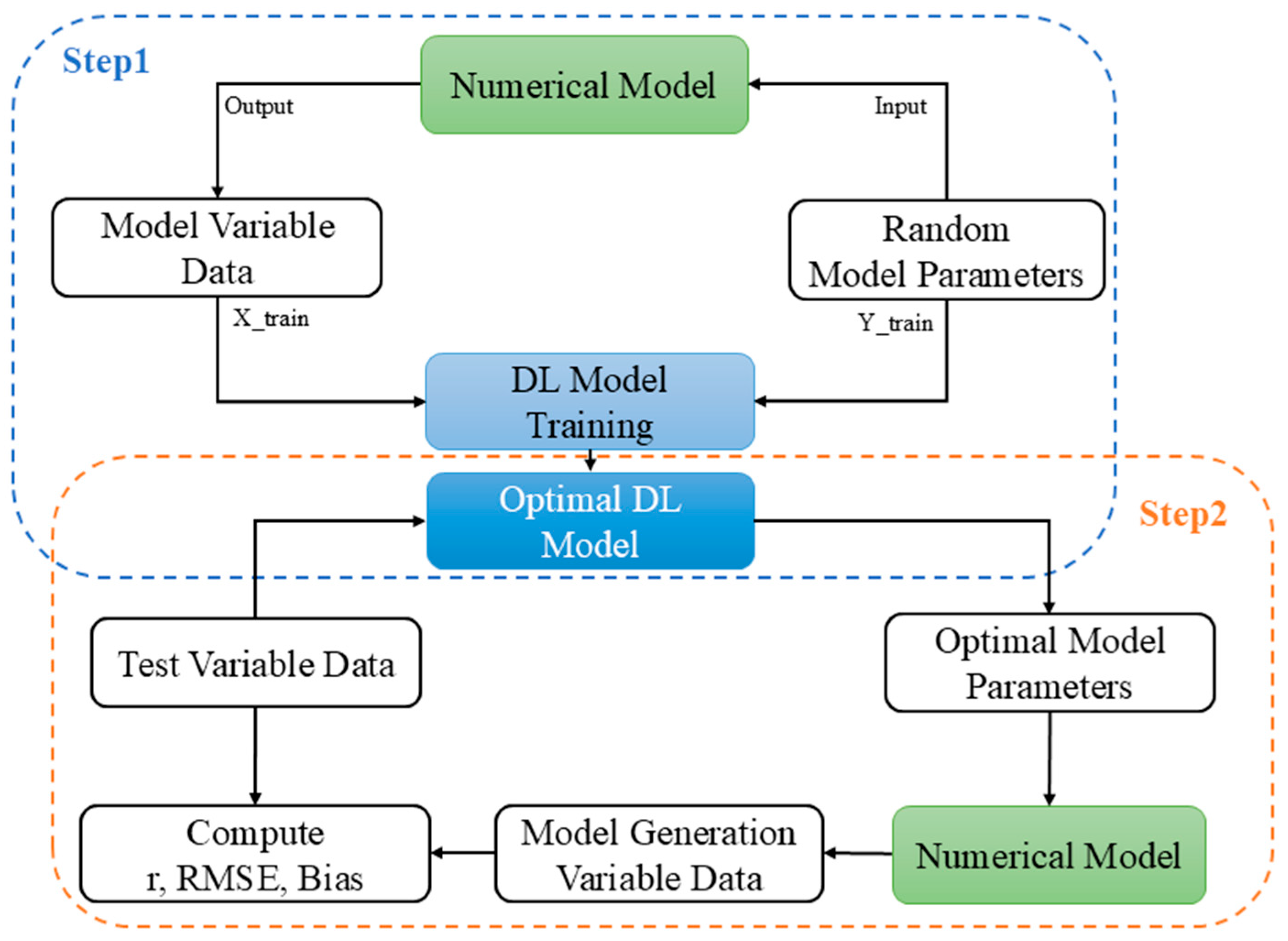
2.3. Deep Learning Framework

In this research, we employed a DL model based on the U-net architecture, which is widely used in image segmentation tasks due to its symmetric encoder–decoder structure and skip connections [36,37]. We utilized the U-net architecture to capture the relationship between ME model variables and ME model parameters, as depicted in Figure 3. The model comprises a U-shaped structure featuring four encoder–decoder modules. To enhance the model’s ability to learn nonlinear relationships, we replaced the traditional ReLU activation function with the Sigmoid Linear Unit (SiLU) activation function, which offers smoother activation characteristics. To combat overfitting and alleviate issues related to exploding or vanishing gradients, Batch Normalization (BN) was applied following the convolutional layers. Additionally, we utilized the AdamW optimizer to enhance training stability and performance through effective weight decay management. Consistent with standard practices in regression tasks, we employed Mean Squared Error Loss (MSELoss) as our loss function.

The basic module of the U-net architecture consists of two 3 × 3 convolutional layers, each followed by a BatchNorm2d layer and a SiLU activation function. The encoder (left half of Figure 3) contains multiple downsampling stages, where each stage reduces the spatial dimensions of the feature maps through max-pooling, enabling the extraction of high-level features. The decoder (right half of Figure 3) mirrors the encoder in structure, performing upsampling operations to gradually restore the spatial resolution and employing skip connections to fuse low-level and high-level features for more accurate representation. A global pooling layer is applied at the end to compress the two-dimensional features into a one-dimensional representation, which is subsequently mapped to 25 model parameters via a fully connected (1 × 1 convolutional) layer.

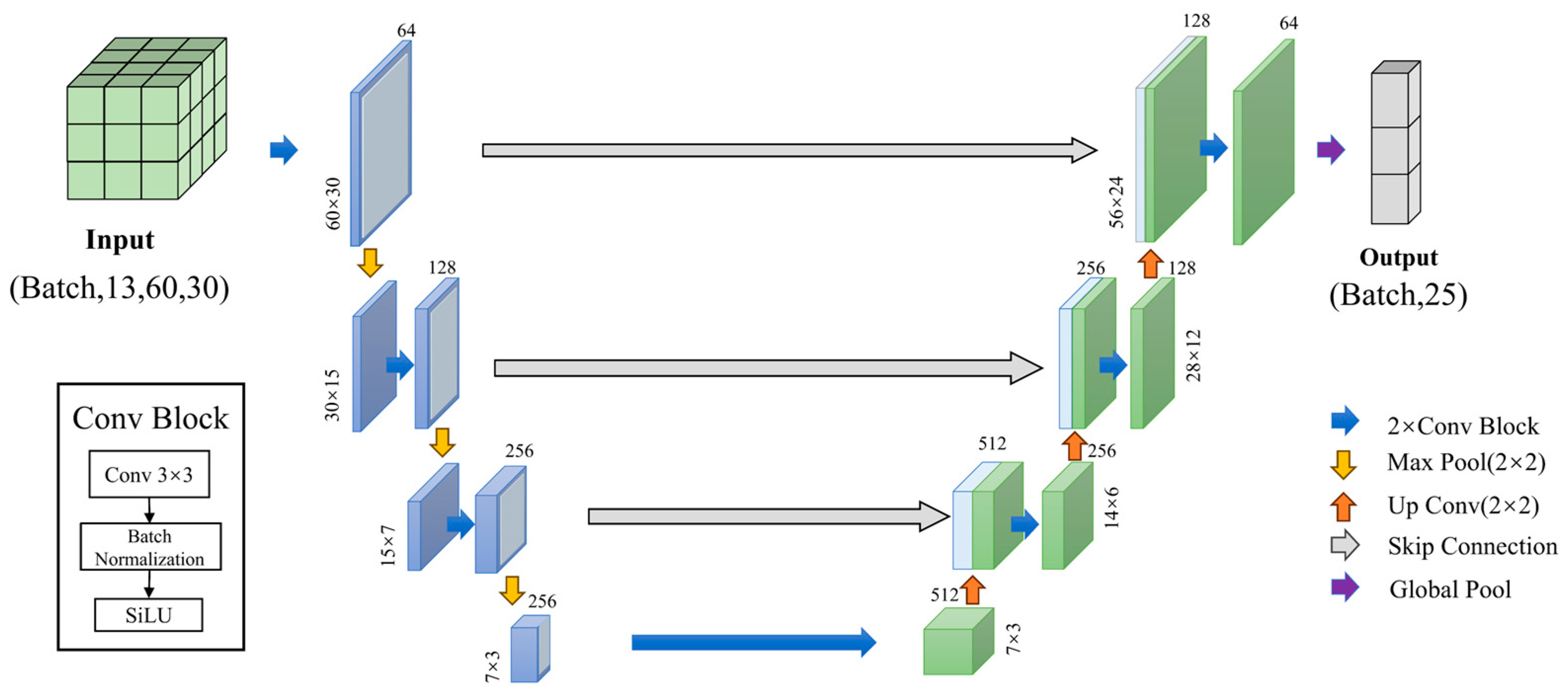
2.4. U-Net Model Training and Evaluation

The U-net model is trained using variable and parameter data, which are randomly generated from the one-dimensional ME model. The training process consists of the following steps:

(1)

Dataset Splitting

A total of 50 sets of variable data (50, 13, 60, 1095) and parameter data (50, 25) are randomly generated from the one-dimensional ME model and are used for U-net model training and evaluation. These datasets are randomly partitioned into training, validation, and testing sets in a 40:7:3 ratio. The training set is used to optimize model parameters; the validation set assists in hyperparameter tuning and early stopping to prevent overfitting; the testing set is used to assess the model’s generalization performance on unseen data.

(2)

Data Preprocessing

To address data limitations and enhance model robustness, the first 15 time steps of the variable data are discarded to eliminate the influence of unstable or unrealistic fluctuations caused by initialization conditions in numerical simulations. The remaining 1080 time steps are then divided into 36 segments. Each segment is represented as a matrix with dimensions [13, 60, 30], where 13 indicates the number of input variables, 60 corresponds to the vertical layers, and 30 represents the number of time steps. These input matrices are processed by the U-net model. All input variables undergo min-max normalization (0–1 scaling) to ensure stable training dynamics. This normalization method rescales each variable to the range [0, 1], calculated using the formula

$$X^{\prime }={\displaystyle \frac{\mathrm{X}-X_{min}}{X_{max}-X_{min}}}$$

(1)

where $\mathrm{X}$ represents the original value, $X_{min}$ and $X_{max}$ denote the minimum and maximum values of the variable, respectively. Min-max normalization ensures that all input features have the same scale, preventing any single variable from dominating the learning process due to differences in magnitude. This helps the model by accelerating convergence, reducing the risk of numerical instability, and improving gradient-based optimization, allowing it to learn more effectively and efficiently.

(3)

Model Training

During model training, the Mean Squared Error (MSE) is used as the loss function to measure the difference between the predicted parameter values and the original numerical model results. The MSE is calculated using the following formula:

$$MSE={\displaystyle \frac{1}{n}}\sum _{i=1}^n{(y_{pre}^i-y_{NM}^i)}^2$$

(2)

where $n$ represents the number of samples, $y_{pre}^i$ denotes the predicted parameters from the AI model output, and $y_{NM}^i$ is the reference parameters from the numerical model.

To improve training efficiency and reduce overfitting, we employed an early stopping strategy. Specifically, training is halted if no decrease in the validation loss is observed over 10 consecutive epochs. Additionally, to further optimize the U-net model’s performance, we implemented a dynamic learning rate adjustment strategy. The initial learning rate is set to 10⁻³, and if the loss on the train set does not decrease within 5 epochs, the learning rate is reduced to one-tenth of its previous value. To prevent the learning rate from becoming too small and halting training, we set a lower bound for the learning rate at 10⁻⁶. The training experiment converged before reaching the preset maximum of 200 epochs, in accordance with the early stopping criteria. The U-net model was realized using the Pytorch toolkit in Python 3.12. The model training takes about 30 min using an NVIDIA 4070Ti GPU (16 GB VRAM), with Windows 11 as the operating system. Once trained, the model can infer a set of parameters within a few seconds.

(4)

Performance Evaluation

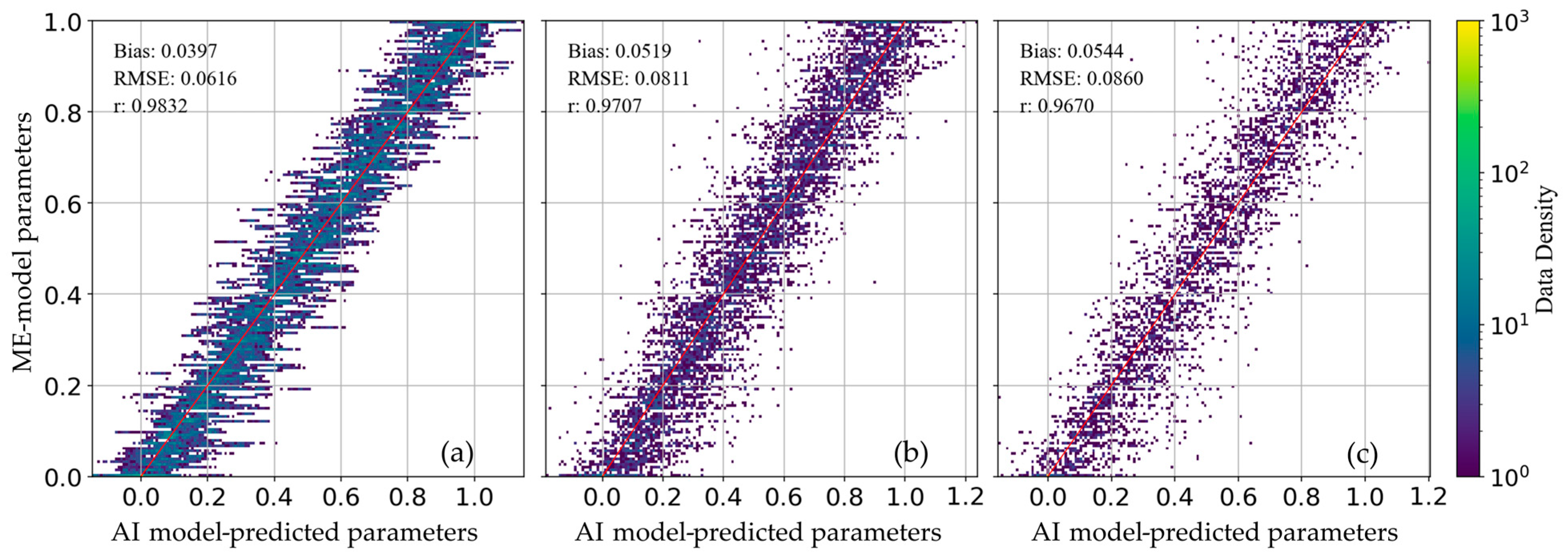
To evaluate accuracy, three key metrics were applied to the training, validation, and test sets: Pearson’s correlation coefficient (r), root mean square error (RMSE), and bias. These metrics provide quantitative measures of the correlation and discrepancies between the predicted parameter data and the original numerical model parameter data. The equations for these metrics are as follows:

$$\mathrm{P}\mathrm{e}\mathrm{a}\mathrm{r}\mathrm{s}\mathrm{o}\mathrm{n}’\mathrm{s} \mathrm{c}\mathrm{o}\mathrm{r}\mathrm{r}\mathrm{e}\mathrm{l}\mathrm{a}\mathrm{t}\mathrm{i}\mathrm{o}\mathrm{n}(\mathrm{r})={\displaystyle \frac{\sum \left(y_i-\bar{y}\right)\left({\widehat{y}}_i-\bar{\widehat{y}}\right)}{\sqrt{\sum {\left(y_i-\bar{y}\right)}^2}\sqrt{\sum {\left({\widehat{y}}_i-\bar{\widehat{y}}\right)}^2}}}$$

(3)

$$\mathrm{RMSE}=\sqrt{{\displaystyle \frac{1}{n}}\sum _{i=1}^n{\left(y_i-{\widehat{y}}_i\right)}^2}$$

(4)

$$\mathrm{Bias}={\displaystyle \frac{1}{n}}\sum _{i=1}^n\left(y_i-{\widehat{y}}_i\right)$$

(5)

where $y_i$ and ${\widehat{y}}_i$ stand for the values of the predicted data and raw data, respectively, and $\bar{y}$ and $\bar{\widehat{y}}$ for their respective means.

3. Results

As shown in Figure 4, we plotted the loss, root mean square error (RMSE), and correlation coefficients (r) of the parameters during model training. The loss and RMSE (Figure 4a,b) curve for the train, validation, and test sets all stabilize after several fluctuations. The consistent trend across all three datasets suggests that the model generalizes well without significant overfitting. Additionally, the correlation coefficient (r) curve in Figure 4c illustrates the alignment between AI model-predicted parameters (U-net model) and numerical model parameters (ME model randomly generates) for all three datasets (train, validation, and test). With an r value around 0.95, the model shows a strong positive correlation, indicating that the AI model-predicted parameter values closely approximate the numerical model parameters. Figure 5 illustrates the scatter plots between the deep learning-predicted parameter results and their corresponding reference True parameter data. To ensure that differences in feature scales do not disproportionately affect the correlation calculations, we standardized the data within the range of [0, 1]. In the scatter plot (Figure 5), the data points from the train, validation, and test sets are evenly distributed on both sides of the optimal fitting line (red line). Furthermore, with both RMSE and bias close to zero, and the correlation coefficient (r) for all datasets exceeding 0.95, this demonstrates that the U-net model effectively captures the underlying relationships between parameters and variables.

Table 3. Comparison of ME model parameters in the test set with parameters inferred by the AI model.

Sequence Number	Parameter Names	Parameter Values
		Group 1		Group 2		Group 3
		ME	AI	ME	AI	ME	AI
1	gmaxs1	2.453	2.521	2.207	2.155	2.515	2.521
2	gmaxs2	2.765	2.920	2.827	2.973	2.657	2.920
3	pis1	1.500	1.341	1.436	1.360	1.017	1.341
4	pis2	0.374	0.108	0.156	0.269	0.105	0.108
5	kno3s1	1.017	0.951	0.574	0.563	1.096	0.951
6	knh4s1	0.371	0.374	0.198	0.188	0.435	0.374
7	kpo4s1	0.231	0.224	0.371	0.351	0.263	0.224
8	kno3s2	1.777	1.760	1.734	1.704	1.703	1.760
9	knh4s2	0.243	0.231	0.418	0.399	0.299	0.231
10	kpo4s2	0.203	0.219	0.368	0.4357	0.389	0.219
11	ksio4s2	4.823	4.825	4.969	4.996	4.843	4.825
12	ak1	0.627	0.619	0.669	0.652	0.655	0.619
13	ak2	0.035	0.034	0.035	0.035	0.033	0.034
14	gammas1	0.039	0.039	0.035	0.035	0.038	0.039
15	gammas2	0.036	0.037	0.028	0.029	0.834	0.846
16	beta1	0.851	0.846	0.841	0.835	0.269	0.256
17	beta2	0.256	0.256	0.275	0.274	0.269	0.256
18	gamma1	0.816	0.810	0.804	0.828	0.829	0.810
19	gamma2	0.492	0.496	0.474	0.475	0.484	0.496
20	gammaz	0.065	0.067	0.055	0.050	0.070	0.067
21	kex1	0.099	0.098	0.061	0.061	0.098	0.098
22	kex2	0.092	0.090	0.099	0.096	0.091	0.090
23	wss2	0.845	0.822	0.946	0.965	0.875	0.822
24	wsdn	0.971	0.966	0.921	0.911	0.965	0.966
25	wsdsi	0.923	0.943	0.967	0.987	0.890	0.943

presents a comparison between the parameters inferred using the U-net model and those obtained from the ME model in the test set. The results show that they are not identical and there are subtle differences. The minor discrepancies observed between the parameters inferred by the U-net model and those derived from the ME model can be attributed to several underlying factors. Firstly, the parameter estimation problem in biogeochemical models is inherently ill-posed, as multiple distinct parameter combinations may produce similar model outputs, a phenomenon commonly referred to as equifinality [38]. Secondly, deep learning models such as U-net are typically trained to minimize a statistical loss function over a given dataset, which leads them to approximate parameter sets that optimize predictive performance, rather than precisely recovering physically meaningful values [39]. Thirdly, due to the strong nonlinearity of the internal processes in marine biogeochemical models, even small perturbations in parameter values can be significantly amplified or attenuated through model dynamics, thereby complicating the exact inversion of the original parameters [40]. Because numerical models can yield the same results from different parameter combinations, to verify whether the numerical model exhibits significant variations in variable outcomes due to slight changes in parameter combinations, we input the parameters (Table 2) predicted by the U-net model back into the numerical model to obtain new variable combinations.

In Figure 6, we present a scatter plot comparing key variable combinations obtained from the numerical model with those simulated variables with AI-inferred parameters (AIPs). The results demonstrate that the AIP simulations for nutrients, zooplankton, and phytoplankton closely match the numerical model outputs, indicating high fidelity. This consistency can be attributed to the accurate numerical representation of fundamental ecological processes, such as phytoplankton primary production and zooplankton grazing, which are well-constrained by multiple parameters within the model [9]. When these parameters are effectively estimated by the deep learning model, the resulting simulations exhibit strong agreement with the reference outputs. However, the correlation coefficient (r) for detritus nitrogen and detritus silicon is slightly lower (~0.9). This discrepancy is likely due to the complex biological origins of detritus in the model, which are predominantly derived from zooplankton excretion and mortality. These processes are often parameterized in simplified forms, making it difficult to capture their full ecological complexity [41]. Consequently, the AI model, despite its capacity for learning nonlinear mappings, may not fully reproduce the intricacies of detritus dynamics, especially when key processes are underrepresented or highly variable in the training data [39]. Overall, while some over- or under-estimations were noted for a subset of data points, the general performance of the AIP simulations remained robust across all state variables, with high correlation values throughout. This suggests that deep learning provides a promising framework for parameter inference in marine biogeochemical models. Nevertheless, the observed discrepancies underscore the challenge of capturing all multivariate dependencies and feedbacks in highly nonlinear ecological systems, particularly when model structures or observational constraints are limited.

4. Discussion

In this study, we developed a deep learning-based parameter estimation method and demonstrated its effectiveness using a one-dimensional ecological numerical model as an example. The results show that our approach significantly streamlines the parameter tuning process by capturing the intricate nonlinear relationships between parameters and variables. A key contribution of this study is the integration of the U-net architecture, which enhances both the efficiency and precision of parameter inference. U-net’s capacity to extract multi-scale spatial features and capture intricate dependencies allows the model to learn from diverse patterns in the data, thereby improving its generalization ability. Efficiency in optimizing parameters for numerical models has been enhanced by leveraging U-net model to swiftly identify the most relevant parameter sets for the numerical model. The proposed method exhibits notable advantages over traditional parameter tuning approaches, as evidenced by the consistently high correlation coefficients (r > 0.95) and the minimal RMSE and bias values observed across the train, validation, and test datasets.

Furthermore, by employing a data-driven approach instead of traditional trial-and-error or gradient-based optimization techniques [24,26,42], our method significantly improves computational efficiency while maintaining precision. Conventional parameter tuning methods often struggle with high-dimensional search spaces and local minima. They typically require sensitivity experiments to assess parameter importance, followed by numerous trials of key parameter combinations to achieve numerical model results that closely approximate real-world data. This parameter tuning approach is not only labor-intensive but also demands extensive domain expertise. Even so, obtaining an optimal parameter set can be highly challenging, especially for complex numerical models. Therefore, our proposed deep learning-based parameter optimization method offers a novel approach to enhancing the efficiency and accuracy of numerical model parameter tuning.

The proposed deep learning-based parameter estimation method is particularly suitable for cases where the fundamental structure of the ecosystem model is well established, such as in widely used coupled physical–biogeochemical models like CoSiNE. These models incorporate key ecological processes (e.g., phytoplankton growth and grazing) through standard formulations, while the associated parameter values are often site-specific, difficult to measure, and exhibit complex nonlinear relationships. In such “structure-known, parameter-unknown” scenarios, our method provides an efficient way to estimate ecologically meaningful parameter sets. Compared to traditional optimization methods, the deep learning framework is better equipped to handle the multi-scale and nonlinear interactions among parameters [43], especially when observational data are limited. While we acknowledge that in some real-world ecosystems both model structure and parameters may be uncertain, many practical applications lie in between. In these semi-known systems, the proposed approach offers a promising tool to enhance model calibration and predictive performance by integrating process-based knowledge with data-driven inference.

Our proposed parameter estimation method, when applied in practice, first requires the construction of a numerical model based on mathematical equations. Next, we utilize deep learning to establish the relationships between variables and parameters within the numerical model, forming an AI-driven parameter estimation framework. Subsequently, we replace the test dataset (as shown in Step 2 of Figure 1) with continuous, long-term observed time series from the real ocean, enabling the retrieval of accurate parameter combinations that reflect real-world conditions. However, due to the sparse and irregular nature of ocean measurements, obtaining complete and continuous 3D ocean observations remains a significant challenge. As a result, our approach is particularly well-suited for 1D numerical experiments, where data continuity is less of a concern, making parameter estimation more feasible. In this study, our proposed approach is to construct statistical models by learning the relationships between input variables and parameters in numerical models through a deep learning framework. The structure and complexity of the deep learning framework can be flexibly adapted to the underlying complexity of the numerical model used. For relatively simple numerical models, lightweight deep learning architectures are sufficient; whereas for more complex and realistic models, deeper and more sophisticated neural networks can be designed accordingly. Thus, this scalability makes the approach applicable not only to theoretical or idealized modeling studies, but also to more complex numerical simulations of ecosystems.

In addition, the computational cost of numerical modeling may present a potential limitation to extending this approach to three dimensions. In this study, we employed a one-dimensional model and randomly generated 50 sets of three-year time series data. The model’s simplification significantly reduced computational burden, making deep learning-based parameters estimation feasible. However, extending this approach to a three-dimensional numerical model would necessitate generating and processing a large volume of high-dimensional time-series datasets, leading to substantial computational demands. The increased complexity and resource requirements could pose challenges for large-scale applications. Nonetheless, the insights gained in this study are important references for refining parameter tuning strategies in more complex numerical modeling frameworks.

In summary, our findings underscore the effectiveness of deep learning in parameter estimation, demonstrating its potential as a robust alternative to conventional methods. The proposed approach not only enhances the reliability of parameter selection but also provides a scalable and automated solution for improving the predictive accuracy of numerical models.

5. Conclusions

In this work, we proposed a deep learning-based parameter optimization method for ecological numerical models, specifically targeting a one-dimensional numerical model. The results show that the method effectively captures the complex relationships between parameters and variables, providing an efficient solution for parameter optimization. The model demonstrated high predictive accuracy, with a correlation coefficient (r) consistently above 0.95 and low bias and RMSE values, confirming the reliability and robustness of the deep learning approach. While the method shows promise, its direct application to three-dimensional numerical models is still constrained by computational demands and data limitations. Future research should focus on improving the scalability and computational efficiency of the method for more complex models.

In conclusion, the deep learning-based parameter optimization method presented in this study offers an effective approach to improving the parameter optimization process in ecological modeling. By providing an automated and efficient solution, it has the potential to advance ecological and biogeochemical modeling, offering an effective method for developing numerical models.

References

1. Gattuso, J.; Magnan, A.; Bopp, L.; Cheung, W.; Duarte, C.; Hinkel, J.; McLeod, E.; Micheli, F.; Oschlies, A.; Williamson, P.; et al. Ocean Solutions to Address Climate Change and Its Effects on Marine Ecosystems. Front. Mar. Sci. 2018, 5, 337. [Google Scholar] [CrossRef]
2. Doney, S.; Ruckelshaus, M.; Emmett Duffy, J.; Barry, J.; Chan, F.; English, C.; Galindo, H.; Grebmeier, J.; Hollowed, A.; Knowlton, N.; et al. Climate Change Impacts on Marine Ecosystems. Annu. Rev. Mar. Sci. 2012, 4, 11–37. [Google Scholar] [CrossRef]
3. Shu, C.; Xiu, P.; Xing, X.; Qiu, G.; Ma, W.; Brewin, R.; Ciavatta, S. Biogeochemical Model Optimization by Using Satellite-Derived Phytoplankton Functional Type Data and BGC-Argo Observations in the Northern South China Sea. Remote Sens. 2022, 14, 1297. [Google Scholar] [CrossRef]
4. Fang, W.; Geng, B.; Xiu, P. Typhoon Effects on the Vertical Chlorophyll Distribution on the Northern Shelf of the South China Sea. J. Geophys. Res. Ocean. 2022, 127, e2022JC019350. [Google Scholar] [CrossRef]
5. Geng, B.; Xiu, P.; Liu, N.; He, X.; Chai, F. Biological Response to the Interaction of a Mesoscale Eddy and the River Plume in the Northern South China Sea. J. Geophys. Res. Ocean. 2021, 126, e2021JC017244. [Google Scholar] [CrossRef]
6. Riley, G.A. Quantitative ecology of the plankton of the western North Atlantic. Bull. Bingham Oceanogr. Collect. 1949, 12, 1–169. [Google Scholar]
7. Heinle, A.; Slawig, T. Internal dynamics of NPZD type ecosystem models. Ecol. Model. 2013, 254, 33–42. [Google Scholar] [CrossRef]
8. Franks, P. NPZ models of plankton dynamics: Their construction, coupling to physics, and application. J. Oceanogr. 2002, 58, 379–387. [Google Scholar] [CrossRef]
9. Fasham, M.; Ducklow, H.; McKelvie, S. A nitrogen-based model of plankton dynamics in the oceanic mixed layer. J. Mar. Res. 1990, 48, 591–639. [Google Scholar] [CrossRef]
10. Allen, J.; Siddorn, J.; Blackford, J.; Gilbert, F. Turbulence as a control on the microbial loop in a temperate seasonally stratified marine systems model. J. Sea Res. 2004, 52, 1–20. [Google Scholar] [CrossRef]
11. Fennel, W. Towards bridging biogeochemical and fish-production models. J. Mar. Syst. 2008, 71, 171–194. [Google Scholar] [CrossRef]
12. Chai, F.; Dugdale, R.; Peng, T.; Wilkerson, F.; Barber, R. One-dimensional ecosystem model of the equatorial Pacific upwelling system. Part I: Model development and silicon and nitrogen cycle. Deep Sea Res. Part II Top. Stud. Oceanogr. 2002, 49, 2713–2745. [Google Scholar] [CrossRef]
13. Xiu, P.; Chai, F. Modeled biogeochemical responses to mesoscale eddies in the South China Sea. J. Geophys. Res. Ocean. 2011, 116, C10006. [Google Scholar] [CrossRef]
14. Guo, L.; Xiu, P.; Chai, F.; Xue, H.; Wang, D.; Sun, J. Enhanced chlorophyll concentrations induced by Kuroshio intrusion fronts in the northern South China Sea. Geophys. Res. Lett. 2017, 44, 11565–11572. [Google Scholar] [CrossRef]
15. Ma, W.; Xiu, P.; Chai, F.; Li, H. Seasonal variability of the carbon export in the central South China Sea. Ocean Dyn. 2019, 69, 955–966. [Google Scholar] [CrossRef]
16. Zhou, F.; Chai, F.; Huang, D.; Xue, H.; Chen, J.; Xiu, P.; Xuan, J.; Li, J.; Zeng, D.; Ni, X. Investigation of hypoxia off the Changjiang Estuary using a coupled model of ROMS-CoSiNE. Prog. Oceanogr. 2017, 159, 237–254. [Google Scholar] [CrossRef]
17. Xiu, P.; Chai, F.; Curchitser, E.N.; Castruccio, F.S. Future changes in coastal upwelling ecosystems with global warming: The case of the California Current System. Sci. Rep. 2018, 8, 2866. [Google Scholar] [CrossRef]
18. Fasham, M. Variations in the seasonal cycle of biological production in subarctic oceans: A model sensitivity analysis. Deep Sea Res. Part I Oceanogr. Res. Pap. 1995, 42, 1111–1149. [Google Scholar] [CrossRef]
19. LöPtien, U.; Dietze, H. Effects of parameter indeterminacy in pelagic biogeochemical modules of Earth System Models on projections into a warming future: The scale of the problem. Glob. Biogeochem. Cycles 2017, 31, 1155–1172. [Google Scholar] [CrossRef]
20. Gharamti, M.; Samuelsen, A.; Bertino, L.; Simon, E.; Korosov, A.; Daewel, U. Online tuning of ocean biogeochemical model parameters using ensemble estimation techniques: Application to a one-dimensional model in the North Atlantic. J. Mar. Syst. 2017, 168, 1–16. [Google Scholar] [CrossRef]
21. Xiao, Y.; Friedrichs, M. The assimilation of satellite-derived data into a one-dimensional lower trophic level marine ecosystem model. J. Geophys. Res. Ocean. 2014, 119, 2691–2712. [Google Scholar] [CrossRef]
22. Mattern, J.; Dowd, M.; Fennel, K. Particle filter-based data assimilation for a three-dimensional biological ocean model and satellite observations. J. Geophys. Res. Ocean. 2013, 118, 2746–2760. [Google Scholar] [CrossRef]
23. Kuroda, H.; Kishi, M. A data assimilation technique applied to estimate parameters for the NEMURO marine ecosystem model. Ecol. Model. 2004, 172, 69–85. [Google Scholar] [CrossRef]
24. Fennel, K.; Losch, M.; Schröter, J.; Wenzel, M. Testing a marine ecosystem model: Sensitivity analysis and parameter optimization. J. Mar. Syst. 2001, 28, 45–63. [Google Scholar] [CrossRef]
25. Doron, M.; Brasseur, P.; Brankart, J. Stochastic estimation of biogeochemical parameters of a 3D ocean coupled physical–biogeochemical model: Twin experiments. J. Mar. Syst. 2011, 87, 194–207. [Google Scholar] [CrossRef]
26. Hoshiba, Y.; Hirata, T.; Shigemitsu, M.; Nakano, H.; Hashioka, T.; Masuda, Y.; Yamanaka, Y. Biological data assimilation for parameter estimation of a phytoplankton functional type model for the western North Pacific. Ocean Sci. 2018, 14, 371–386. [Google Scholar] [CrossRef]
27. Marjorie, A.; Raleigh, R.; Jerry, D. Ecosystem model complexity versus physical forcing: Quantification of their relative impact with assimilated Arabian Sea data. Deep Sea Res. Part II Top. Stud. Oceanogr. 2006, 53, 576–600. [Google Scholar]
28. Hittawe, M.; Harrou, F.; Sun, Y.; Knio, O. Stacked Transformer Models for Enhanced Wind Speed Prediction in the Red Sea. In Proceedings of the 2024 IEEE 22nd International Conference on Industrial Informatics (INDIN), Beijing, China, 18–20 August 2024; pp. 1–7. [Google Scholar]
29. LeCun, Y.; Bengio, Y.; Hinton, G. Deep learning. Nature 2015, 521, 436–444. [Google Scholar] [CrossRef]
30. Afzal, S.; Hittawe, M.M.; Ghani, S.; Jamil, T.; Knio, O.; Hadwiger, M.; Hoteit, I. The state of the art in visual analysis approaches for ocean and atmospheric datasets. Comput. Graph. Forum 2019, 38, 881–907. [Google Scholar] [CrossRef]
31. Toni, T.; Welch, D.; Strelkowa, N.; Ipsen, A.; Stumpf, M.P. Approximate Bayesian computation scheme for parameter inference and model selection in dynamical systems. J. R. Soc. Interface 2009, 6, 187–202. [Google Scholar] [CrossRef]
32. Gutenkunst, R.; Waterfall, J.; Casey, F.; Brown, K.; Myers, C.; Sethna, J. Universally sloppy parameter sensitivities in systems biology models. PLoS Comput. Biol. 2007, 3, e189. [Google Scholar] [CrossRef]
33. Wang, Z.; Chai, F. CoSiNE Manual; Virginia Institute of Marine Science: Gloucester Point, VA, USA, 2017; p. 16. Available online: https://ccrm.vims.edu/schismweb/CoSiNE_manual_ZG_v5.pdf (accessed on 15 June 2025).
34. Kishi, M.J.; Kashiwai, M.; Ware, D.M.; Megrey, B.A.; Eslinger, D.L.; Werner, F.E.; Noguchi-Aita, M.; Azumaya, T.; Fujii, M.; Hashimoto, S. NEMURO—A lower trophic level model for the North Pacific marine ecosystem. Ecol. Model. 2007, 202, 12–25. [Google Scholar] [CrossRef]
35. Evans, G.T.; Parslow, J.S. A model of annual plankton cycles. Biol. Oceanogr. 1985, 3, 327–347. [Google Scholar]
36. Wang, J.; Chen, J.; Chen, D.; Wu, J. LKM-UNet: Large Kernel Vision Mamba Unet for Medical Image Segmentation. In Proceedings of the Medical Image Computing and Computer Assisted Intervention—MICCAI 2024, Marrakesh, Morocco, 6–10 October 2024; pp. 360–370. [Google Scholar]
37. Ronneberger, O.; Fischer, P.; Brox, T. U-net: Convolutional Networks for Biomedical Image Segmentation. In Proceedings of the Medical Image Computing and Computer-Assisted Intervention—MICCAI 2015: 18th international conference, Munich, Germany, 5–9 October 2015; pp. 234–241. [Google Scholar]
38. Luo, Y.; Weng, E.; Wu, X.; Gao, C.; Zhou, X.; Zhang, L. Parameter identifiability, constraint, and equifinality in data assimilation with ecosystem models. Ecol. Appl. 2009, 19, 571–574. [Google Scholar] [CrossRef] [PubMed]
39. Reichstein, M.; Camps-Valls, G.; Stevens, B.; Jung, M.; Denzler, J.; Carvalhais, N.; Prabhat, F. Deep learning and process understanding for data-driven Earth system science. Nature 2019, 566, 195–204. [Google Scholar] [CrossRef]
40. Simon, W. Statistical inference for noisy nonlinear ecological dynamic systems. Nature 2010, 466, 1102–1104. [Google Scholar]
41. Anderson, T.; Pondaven, P. Non-redfield carbon and nitrogen cycling in the Sargasso Sea: Pelagic imbalances and export flux. Deep Sea Res. Part I Oceanogr. Res. Pap. 2003, 50, 573–591. [Google Scholar] [CrossRef]
42. Ji, X.; Liu, G.; Gao, S.; Wang, H. Parameter sensitivity study of the biogeochemical model in the China coastal seas. Acta Oceanol. Sin. 2015, 34, 51–60. [Google Scholar] [CrossRef]
43. Hemmings, J.; Challenor, P.; Yool, A. Mechanistic site-based emulation of a global ocean biogeochemical model (MEDUSA 1.0) for parametric analysis and calibration: An application of the Marine Model Optimization Testbed (MarMOT 1.1). Geosci. Model Dev. 2015, 8, 697–731. [Google Scholar] [CrossRef]
Figure 1. Schematic diagram of the overall workflow.
Jmse 13 01228 g001
Figure 2. CoSiNE-13 model framework diagram. The boxes of different colors in the diagram represent all variables in the CoSiNE-13 model. The blue dashed boxes indicate the production and consumption processes of dissolved oxygen. The black arrows represent the direction of material flow and transformation (e.g., uptake, excretion, remineralization), the blue double-headed arrows denote air-sea exchange fluxes, and the red arrows represent the photosynthesis process.
Jmse 13 01228 g002
Figure 3. An illustration of the U-net architecture used in this study. Each colored cube symbolizes a feature map, with the numbers on the sides indicating the width × height dimensions, and the numbers at the top representing the number of channels.
Jmse 13 01228 g003
Figure 4. (a) Loss; (b) RMSE; (c) r curves for train, validation, and test datasets.
Jmse 13 01228 g004
Figure 5. Scatter plots between AI model-predicted parameter results and their corresponding reference parameter data, (a) train set; (b) validation set; (c) test set.
Jmse 13 01228 g005
Figure 6. Scatter plots between simulated variables with AI-inferred parameters and their corresponding reference variable ME model variable in test set, (a) NO3; (b) PO4; (c) SiO4; (d) NH4; (e) S2; (f) Z2; (g) DOX; (h) DN; (i) DSi.
Jmse 13 01228 g006