Temperature-Induced Errors in ITTC Model-Ship Extrapolation

Abstract

This study addresses the question: “Does the towing tank water temperature affect the result of model-ship extrapolation?” While it is well-established that temperature variations affect Reynolds numbers and consequently frictional and viscous resistance, this study examines whether the ITTC 1978 extrapolation method properly compensates for these effects. Although current procedures consider temperature indirectly through the Reynolds number, they assume that the form factor depends solely on the Froude number and is insensitive to viscosity changes. Our analysis reveals that the form factor is also temperature-sensitive, indicating a fundamental limitation in the conventional approach. This sensitivity arises from the limitations of the ITTC 1957 friction curve and the method’s neglect of temperature-induced variations in the form factor. To quantify the effect of temperature, model-scale CFD simulations were conducted for two ship models (KCS and KVLCC2) at different water temperatures using the ITTC 1978 procedure with Prohaska’s method. The results show that the ship-scale total resistance coefficient ($C_T$) can vary by up to 2.8% depending on the water temperature and friction line selection. This demonstrates that the ITTC 1978 performance prediction method fails to adequately compensate for the temperature-induced changes in resistance, which leads to systematic errors in the extrapolated results.

1. Introduction

With the acceleration of global warming driven by increased carbon emissions, global efforts are underway to develop eco-friendly and decarbonisation technologies. The International Maritime Organisation (IMO), which oversees maritime regulations, has introduced its net zero plan, aiming to neutralise carbon emissions from ships by 2050 [1].

Ship performance prediction is one of the most important tasks during the design process for ships. In addition, legal authorities require towing tank testing in ship evaluations, particularly for calculating factors such as the Energy Efficiency Design Index (EEDI), which has been enforced by the IMO since 2011.

In the maritime industry, accurate ship resistance prediction is crucial for optimising vessel performance and fuel efficiency. Historically, towing tank testing has been the predominant method for accurately predicting ships’ performance in deep and calm waters, tracing back to William Froude’s pioneering work on extrapolation procedures in the 1870s. Although towing tank testing has been historically reliable, advancements have emerged over time to enhance and refine these conventional practices. Despite decades of debate, discussion, and improvement regarding towing tank testing and extrapolation methods, inherent and well-known shortcomings persist due to scale effects [2].

A recent study [3] has highlighted ongoing challenges associated with extrapolation procedures in ship hydrodynamics, including persistent uncertainties and the limitations of traditional model testing. Despite advancements in computational fluid dynamics (CFD) that were aimed at mitigating these issues, the review emphasises that the naval architecture community is not yet ready to fully replace experimentation with CFD. Furthermore, Song et al. highlighted that, while CFD simulations can closely predict the model-scale resistance, the full-scale resistance predictions must account for the effects of hull roughness [4]. They demonstrated this by cross-validating their full-scale CFD simulations and the ITTC (International Towing Tank Conference) 1978 method with Townsin’s formula.

A significant development occurred in 1973 with the creation of computer programs by SSPA Sweden AB in response to requests from the ITTC [5]. These programs introduced innovative assumptions and extrapolation methods, ushering in a more standardised and technologically driven approach to ship performance prediction. While towing tank testing remains fundamental in understanding ship behaviour, modern computational tools, such as computational fluid dynamics (CFD), have emerged as effective and efficient methods for simulating ship performance under various conditions. CFD has been positioned as a promising alternative to traditional methods [2,6,7]. This transition towards CFD seemed apparent due to its capability to satisfy both Froude and Reynolds similarities, which are fundamentally impossible to satisfy in single model experiments due to the different scaling behaviours of inertial and viscous forces. Moreover, the advancements in computational power and modelling techniques in recent years have enabled more accurate and detailed simulations of complex fluid dynamics around ship hulls. Consequently, CFD has become a valuable tool for optimising ship design and performance, complementing, and sometimes surpassing, the capabilities of traditional towing tank testing.

However, despite these advancements, towing tank tests continue to play a vital role in the evaluation and optimisation of hull form designs. These tests rely on the ITTC 1978 performance prediction method, which employs the ITTC 1957 correlation line. The ITTC 1957 curve, which was originally adapted from the Kármán–Schoenherr formula (i.e., ATTC curve), was aimed to reconcile the results of large and small models. It was proposed as an interim solution due to the limitations of the existing Kármán–Schoenherr curve at low Reynolds numbers and the inconvenience of its implicit form. The ITTC friction curve provides a better correlation for ship resistance predictions, particularly in situations where the Kármán–Schoenherr curve’s limitations pose challenges for calculations [8]. As this correlation line was empirically derived from historical towing tank tests, it inherently includes experimental uncertainties—such as the instrumentation accuracy, flow control, and boundary conditions—that may affect its predictive fidelity.

Efforts to address the limitations of the ITTC 1957 friction curve are ongoing, as it has been the standard for extrapolating model-ship resistance to full-scale ships. Possible issues with this curve have prompted the exploration of other alternatives to improve the accuracy of ship resistance predictions. Granville showed that the ITTC 1957 correlation curve can also be considered as a turbulent flat frictional resistance curve [9]. From fundamental considerations involving the velocity distribution in the boundary layer, he derived the general formula. Grigson’s friction curve [10] provided a refined approach to calculating ship resistance by incorporating a more detailed analysis of turbulent flow characteristics. It considered the complex behaviour of turbulent boundary layers and the transition from laminar to turbulent flow, which are critical factors in accurately predicting frictional resistance.

Over the past two decades, discussions regarding the ITTC 1957 friction curve have been sparked by recent developments. Of these, discussions related to the 23rd, 25th, and 29th ITTC committees raised concerns about the accuracy of this correlation line. In the 23rd ITTC propulsion committee [11], the discrepancies between full-scale and model-scale form factors calculated using $C_F$ from the ITTC 1957 correlation line were mentioned. This discrepancy, which is about 1/3 higher at full scale relative to at model scale, raises questions about the accuracy of the ITTC 1957 friction curve as an accurate friction formula. The 25th ITTC resistance committee [12], once again, questioned the validity of the existing ITTC friction curve for a wider range of Reynolds numbers, and recommended the development of a new friction formula. Different flat plate friction lines have been suggested with the intention of offering improved accuracy over the ITTC 1957 correlation curve. Katsui et al. proposed a new friction line for flat plates [13]. This equation was derived from differential equations, including the momentum integral equation and Coles’ wall-wake law. It addresses limitations of the ITTC 1957 friction curve such as its speed dependence and inconsistencies in form factor. Subsequently, in the powering performance committee of the 25th ITTC [12], total resistance data for full-scale ships were analysed, which highlights the ongoing debate surrounding the ITTC 1957 friction line.

At the ITTC 29th conference [14], issues were discussed, with key points including that the combined use of experiments and CFD improves the accuracy of resistance predictions, and that further studies are needed before a new model-ship correlation line can be introduced or the ITTC 1957 friction curve revisited. Therefore, the ITTC 29th conference highlighted ongoing concerns about the limitations of the ITTC 1957 correlation line, which emphasised the need for further research before any revisions are made.

Recent studies in the realm of friction curves have explored various approaches to enhancing their accuracy and applicability. Park utilised different friction curves for ship performance prediction and demonstrated the significant role of friction curves in estimating the speed performance of ships in model tests [15]. Wang et al. delved into the refinement of friction curves for flat plate regression through numerical simulations by employing the Reynolds-averaged Navier–Stokes (RANS) method with the SST k-ω turbulence model [16]. Their study emphasised the significance of grid refinement and inlet turbulence energy adjustments in achieving precise predictions, particularly noting discrepancies with traditional friction lines, especially for appended hulls.

Zeng et al. proposed a numerical friction curve to address the effects of shallow water on ship bottoms using CFD calculations [17]. They identified scale effects and the invalidity of the zero-pressure gradient assumption in extremely shallow water, highlighting limitations in the ITTC 1957 correlation line. Korkmaz et al. examined the influence of turbulence models and boundary conditions on numerically derived friction curves across a wide range of Reynolds numbers [18]. By focusing on the broader impact of these factors on CFD-based extrapolation, their research contributed valuable insights into the complexities of friction curve modelling in CFD. Additionally, Korkmaz et al. emphasised the constraints of the ITTC 1978 power prediction method, particularly the contraints in its form factor approach, and proposed a CFD/EFD method to improve ship resistance prediction [2]. These studies demonstrate how CFD can provide a more precise understanding on the behaviour of model-ship extrapolation that is not achievable through traditional model testing.

Table 1. Discussions on the ITTC 1957 friction curve and/or the ITTC 1978 performance prediction method.

Discussion By	Discussion	Suggestion
Granville [9]	ITTC 1957 correlation curve can be considered as a turbulent flat frictional resistance curve	General formula, $C_F={\displaystyle \frac{0.0776}{({Re-1.88)}^2}}+{\displaystyle \frac{60}{Re}}$
Grigson [10]	Concerns about the accuracy of the curve and introduced the Grigson formula as a potential alternative	Grigson formula, (see Equations (12) and (13))
ITTC [11]	Doubts raised about the validity due to discrepancies between full-scale and model-scale form factors
Katsui et al. [13]	Doubts about the friction line include speed dependence and inconsistency in form factor	Katsui equation, (see Equation (14))
ITTC [12]	Analytical studies were conducted for the discussion and recommendation of new friction formulas
Wang et al. [16]	Doubts stem from the friction curve’s inability to accommodate scale-dependent form factor variations	Introduction of a new friction curve (using RANS method)
Zeng et al. [17]	Limitations in the friction curve include a lack of consideration for shallow water effects on ship bottoms	Introduction of a new numerical friction line (using BSL k-ω turbulence)
Korkmaz et al. [2]	Scale effects due to the friction curve contradict Reynolds number independence hypothesis	Introduction of a new numerical friction line (using SST k-ω turbulence)
ITTC [14]	Further studies needed before revising ITTC 1957 friction curve or introducing new correlation line
Korkmaz et al. [18]	Emphasises the constraints of the from factor approach in the ITTC 1978 power prediction method	Form factor replacement with CFD/EFD

provides a summary of the discussions and research related to the ITTC 1957 friction line and the ITTC 1978 performance prediction method.

With the recent advancements in CFD technology, it has become possible to predict the $C_T$ (total resistance coefficient) and $C_F$ (frictional resistance coefficient) with high accuracy in fluid flow simulations. However, the ITTC 1978 method, which is traditionally used during the ship design phase for model-ship extrapolation, has potential limitations. As noted in Table 1, uncertainties surrounding the ITTC 1957 correlation line have persisted. One possible issue is its failure to represent changes in the $C_F$ that result from variations in the Reynolds number. These variations are often caused by changes in the towing tank water temperature. If the ITTC friction curve does not accurately predict the $C_F$ based on the towing tank water temperature, this discrepancy can lead to inaccurate extrapolated resistance values at the ship scale. To address these concerns, the present study performed model-scale CFD simulations under various towing tank water temperature conditions. This involved utilising density and dynamic viscosity parameters that are specific to different temperature settings, and these were sourced from reputable references such as ITTC reports [19].

Therefore, this study aims to analyse the effects of towing tank water temperature variations on model-ship extrapolation and verify the reliability of the ITTC 1957 friction curve for use in current extrapolation methods. Rather than simply analysing the effects of the temperature on ship resistance, this study uses CFD to model how variations in the towing tank water temperature influence the resistance predictions. By addressing the technical challenge of understanding and resolving ship resistance variations with water temperature, this research seeks to enhance the accuracy of ship resistance predictions (specifically $C_T$) and support more reliable decision-making in ship design and operation [20,21].

In this context, the objective of this study is not to validate or improve the ITTC 1957 friction line, but rather to examine how the current ITTC extrapolation procedure behaves under varying towing tank temperatures. Since the ITTC correlation line is still widely used in real-world resistance tests, understanding its limitations in practical applications is essential for accurate performance prediction.

The remainder of this paper is organised as follows.

-

Section 2 presents the methodology and numerical setup, including the implementation of temperature-dependent conditions within the CFD framework;

-

Section 3 presents the results, including verification and validation using the KRISO Container Ship (KCS) and Very Large Crude Carrier (KVLCC2) as validation cases;

-

Section 4 offers a detailed discussion of the results in the broader context of ship hydrodynamics;

-

Finally, Section 5 summarises the conclusions and outlines the limitations and future perspectives of this study.

2. Materials and Methods

2.1. Approach

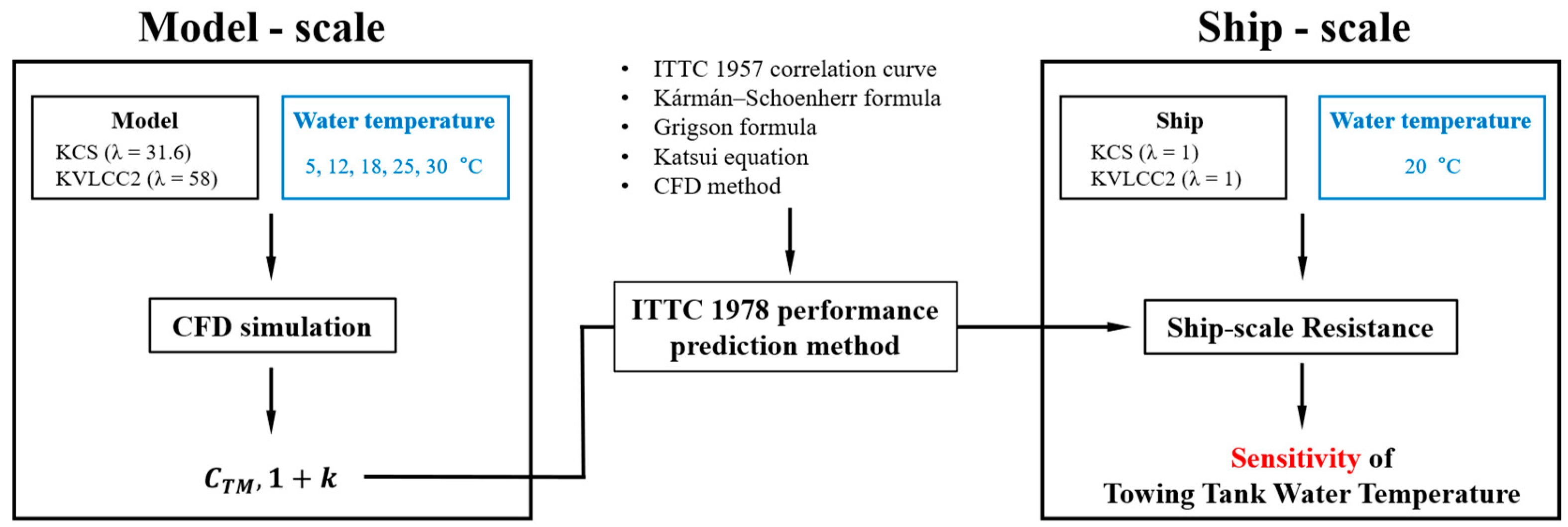
Figure 1 schematically illustrates the methodology utilised in this research. The approach involved conducting computational fluid dynamics (CFD) simulations using two model ships, KCS and KVLCC2, under varied towing tank water temperature conditions (5 °C, 12 °C, 18 °C, 25 °C, and 30 °C). This was accomplished utilising the commercial CFD software STAR-CCM+ (version 18.06).

Additionally, Prohaska’s method [22] was applied at each towing tank temperature condition to derive the form factor values necessary for the model-ship extrapolation. These form factors were then used to estimate ship resistance, following the ITTC 1978 performance prediction method. This was calculated using five distinct friction curves: the ITTC 1957 correlation curve, the ATTC friction curve (also known as Kármán–Schoenherr formula), the Grigson formula, the Katsui equation, and an imaginary $C_F$ curve that precisely matches the $C_F$ values derived from CFD simulations. It is important to note that the water temperature at the ship scale remained constant at 20 °C throughout all conditions. Lastly, this study examined the sensitivity of towing tank water temperatures by comparing the results obtained from the five different friction curves.

2.2. ITTC 1978 Model-Ship Extrapolation

The total resistance, $R_T$, of a ship can be separated into two primary components: the frictional resistance, $R_F$, and the residuary resistance, $R_R$, which can be expressed as follows:

$$R_T=R_F+R_R$$

(1)

Frictional resistance results from the friction between the fluid and the hull surface, while the residuary resistance is a pressure-related resistance that includes the viscous pressure resistance, $R_{VP}$, and wave-making resistance, $R_W$, as given by the following:

$$R_T=R_F+R_{VP}+R_W$$

(2)

Viscous pressure resistance is generally assumed to be proportional to frictional resistance [23], with the form factor, $k$, as shown below:

$$R_{VP}={kR}_F$$

(3)

The form factor, $k$, is crucial for accurate resistance prediction [24]. The ITTC 1978 model-ship extrapolation method recommends determining the form factor from low-speed tests using Prohaska’s method [22]. These low-speed tests are typically part of the standard resistance tests.

Thus, the total resistance equation becomes the following:

$$R_T={(1+k)R}_F+R_W$$

(4)

Each resistance component can be normalised by dividing it by the dynamic pressure, $\frac{1}{2}\rho S{V}^2$, and the wetted surface area of the ship hull, $S$. This allows the resistance coefficients to be defined as follows:

$$C_T={(1+k)C}_F+C_W$$

(5)

where $C_T, C_F, C_W$ are the coefficient of the total, frictional, and wave-making resistance, respectively. Expanding on these foundations, the ITTC 1978 model-ship extrapolation is intended to disaggregate and rectify the various components that contribute to resistance in ship design. This methodology aims to predict the total resistance of a ship by considering factors such as frictional resistance, form factor adjustments, and wave-making resistance.

The total resistance coefficient for a ship, $C_{TS}$, is expressed as follows:

$$C_{TS}={(1+k)C}_{FS}+C_W+\mathsf{\Delta }{C}_F+C_A+C_{AAS}$$

(6)

Here, $\mathsf{\Delta }{C}_F$ is the roughness allowance, $C_A$ is the correlation allowance, and $C_{AAS}$ is the air resistance coefficient at the ship scale. The wave-making resistance coefficient, $C_W$, is consistent for both the model and the ship, and is derived as follows:

$$C_W=C_{TM}-\left(1+k\right)C_{FM}$$

(7)

The roughness allowance, correlation allowance, and air resistance coefficient were not utilised in this study. Equation (5) presents the simplified ITTC 1978 model-ship extrapolation formula used in this study. Additionally, the form factor derived from Prohaska’s method was applied, and the same value was used for both the model and the ship scales.

2.3. Governing Equation

The CFD models were formulated utilising the unsteady Reynolds-averaged Navier–Stokes (URANS) method within the framework of a commercial CFD software, STAR-CCM+ (version 18.06). This method was selected for its capability to efficiently model turbulent flows and capture unsteady phenomena, which provides a practical approach for engineering simulations. Although the steady RANS is often sufficient for basic resistance prediction, the URANS was employed in this study to capture possible low-frequency unsteady flow features—such as vortex shedding and wake fluctuations—particularly around intermediate Froude numbers (e.g., Fr ≈ 0.26 for KCS), where such effects have been observed in experiments.

The governing equations for incompressible flows, namely the continuity and momentum equations, were expressed in tensor notation and Cartesian coordinates. These equations form the basis of the computational framework, which allows for the simulation of fluid behaviour based on the fundamental principles of conservation laws and fluid dynamics [25].

The continuity equation, Equation (8), ensures mass conservation within the flow domain. Here, $\rho$ represents fluid density and $u_i$ denotes the velocity components in Cartesian coordinates. The momentum equation, given by Equation (9), represents the balance of forces acting on fluid particles. In this equation, $P$ stands for pressure, $\mu$ is dynamic viscosity, $S_{ij}$ denotes the strain-rate tensor, and $\rho \underset{\_}{u_i^{\prime }{u}_j^{\prime }}$ represents the Reynolds-stress tensor, which accounts for turbulent fluctuations in velocity. The strain-rate tensor $S_{ij}$, as represented in Equation (10), quantifies the local deformation of fluid elements within the flow field. It captures the rate of change of velocity gradients in different directions, reflecting the stretching and shearing of fluid particles. Additionally, Equation (11) describes the specific Reynolds stress tensor $\rho {\tau }_{ij}$. This tensor contributes to turbulent momentum transfer within the flow field.

$${\displaystyle \frac{\partial \left(\rho u_i\right)}{\partial x_i}}=0$$

(8)

$$\rho {\displaystyle \frac{\partial \left(u_i\right)}{\partial t}}+\rho u_j{\displaystyle \frac{\partial u_i}{\partial x_j}}=-{\displaystyle \frac{\partial P}{\partial x_i}}+{\displaystyle \frac{\partial }{\partial x_j}}\left(2\mu S_{ij}-\rho \underset{\_}{u_i^{\prime }{u}_j^{\prime }}\right)$$

(9)

$$S_{ij}={\displaystyle \frac{1}{2}}\left({\displaystyle \frac{\partial u_i}{\partial x_j}}+{\displaystyle \frac{\partial u_j}{\partial x_i}}\right)$$

(10)

$$\rho {\tau }_{ij}=-\rho \underset{\_}{u_i^{\prime }{u}_j^{\prime }}$$

(11)

The computational domain was discretised using a finite volume method, which subdivided it into a finite number of control volumes. These control volumes facilitate the numerical approximation of the governing equations and enable their calculation over the entire computational domain.

For discretisation, a second-order upwind convection scheme and first-order temporal discretisation were employed for the momentum equations. This approach ensures accurate representation of flow physics, particularly in regions with high velocity gradients and turbulence.

The solution strategy adopted a semi-implicit method for pressure-linked equations (SIMPLE)-type algorithm, which iteratively solves the coupled continuity and momentum equations to obtain the velocity field and momentum equations, allowing us to obtain the velocity field and pressure distribution within the domain. This iterative process continues until a converged solution is achieved, ensuring numerical stability and accuracy.

To accurately capture the free surface behaviours, the volume of fluid (VOF) method, with high-resolution interface capturing (HRIC), was employed [26,27]. This approach accurately tracks the interfaces between fluid phases, allowing for precise representation of free surface phenomena such as wave propagation and surface tension effects.

2.4. Computational Domain and the Boundary Conditions of the KCS and KVLCC2 Hull Simulation

Figure 2 shows the hull geometries of the KCS and KVLCC2 models used in this study. It is of note that KCS includes a rudder, while KVLCC2 does not, which is consistent with the standard definitions provided in [28,29,30].

The computational domain and boundary conditions for simulating the KCS and KVLCC2 hulls were established to ensure accurate representation of their dynamic behaviour, as depicted in Figure 3. The ship hull region was configured with two degrees of freedom (heave and pitch motion) to account for all exerted forces and moments. This comprehensive setup ensured an accurate representation of the vessel’s dynamic behaviour, which is crucial for capturing realistic hydrodynamic responses.

Velocity inlet conditions were applied at the inlet, top, and bottom boundaries to ensure stable inflow. The top and bottom were specifically treated this way to enhance numerical stability and prevent pressure buildup near domain edges. To minimise their influence, vertical clearances of 1.5 L (top) and 3.0 L (bottom) were applied. The outlet was defined as a pressure outlet to allow smooth fluid outflow. A symmetry plane was imposed at the centre midplane to reduce computational cost while preserving accuracy.

Table 2. Principal particulars and conditions of the KCS simulations, adapted from [28,29].

Main Particulars	Ship Scale	Model Scale
Scale factor, $\lambda$	1	31.6
Length between the perpendiculars, $L_{pp}$ ($\mathrm{m}$)	230.0	7.279
Length of the waterline, $L_{wl}$ ($\mathrm{m}$)	232.5	7.357
Beam at the waterline, $B_{wl}$ ($\mathrm{m}$)	32.2	1.019
Design draught, $T$ ($\mathrm{m}$)	10.8	0.342
Wetted surface area with a rudder, $S$ (${\mathrm{m}}^2)$	9645	9.659
Displacement, $\nabla$ (${\mathrm{m}}^3$)	52,030	1.649
Block coefficient, $C_B$	0.651	0.651
Design speed, $V$ ($\mathrm{m}/\mathrm{s}$)	12.346	2.196
Froude number at the design speed, $F_r$	0.260	0.260

and

Table 3. Principal particulars and conditions of the KVLCC2 simulations, adapted from [28,30].

Main Particulars	Ship Scale	Model Scale
Scale factor, $\lambda$	1	31.6
Length between the perpendiculars, $L_{pp}$ ($\mathrm{m}$)	320.0	5.517
Length of the waterline, $L_{wl}$ ($\mathrm{m}$)	325.5	5.612
Beam at the waterline, $B_{wl}$ ($\mathrm{m}$)	58.0	1.0
Design draught, $T$ ($\mathrm{m}$)	20.8	0.359
Wetted surface area with a rudder, $S$ (${\mathrm{m}}^2)$	27,194	8.084
Displacement, $\nabla$ (${\mathrm{m}}^3$)	312,622	1.602
Block coefficient, $C_B$	0.8098	0.8098
Design speed, $V$ ($\mathrm{m}/\mathrm{s}$)	7.9732	1.047
Froude number at the design speed, $F_r$	0.142	0.142

outline the essential characteristics and operating conditions of the KCS and KVLCC2 simulations, which were sourced from [28,29,30]. They include geometric details like length, breadth, and draft. These tables served as a foundation for setting up accurate CFD simulations, ensuring realistic representation of the KCS and KVLCC2 models and their hydrodynamic behaviour.

2.5. Mesh Generation

The mesh for the simulations was generated using the automated mesher in STAR-CCM+, employing the Cartesian cut-cell method. This technique was chosen for its efficiency in handling complex geometries and its ability to produce high-quality meshes, which makes it particularly suitable for ship hull modelling.

The grid structures used in the CFD simulations are illustrated in Figure 4 and Figure 5. A key consideration in mesh generation was maintaining the wall y+ value above 30 to ensure accurate resolution of near-wall flow dynamics and to avoid numerical instability [31]. Grid refinement was applied in the free surface region, particularly in areas where complex wave interactions occur. This refinement enhanced the accuracy of wave-related predictions while preserving appropriate boundary layer resolution without over-refining near the wall.

To confirm that wall y+ values do not significantly affect the simulation results, additional CFD runs were performed for the KVLCC2 model with y+ values below 1, across different towing tank temperatures. All other simulation parameters, including time step, mesh resolution, and form factor application, were kept consistent. A comparison between the high- and low-y+ cases revealed no meaningful differences in the extrapolated resistance results. Further details are provided in Appendix A.

Despite varying temperature conditions, consistent mesh configurations were employed across all simulations to ensure computational consistency and facilitate direct comparisons between scenarios. Furthermore, the mesh was adjusted to ensure consistent wall y+ values across various model types and temperatures. This consistency is reflected in the simulations, where the mesh maintains consistent wall y+ levels across all temperatures used in the CFD simulations for both the KCS and KVLCC2 cases, not just for the low temperature (i.e., 5 °C) and high temperature (i.e., 30 °C).

To achieve these consistent wall y+ values, the first cell thickness was adjusted according to the water temperature. The first cell thickness is a critical parameter in CFD that determines the resolution of the boundary layer near the wall.

Table 4. Mean wall y+ and first cell thickness values for KCS and KVLCC2 at different water temperatures (°C).

Ship		Water Temperature
		5 °C	12 °C	18 °C	25 °C	30 °C
KCS	Mean wall y+	50.69	51.13	51.57	52.04	52.47
	First cell thickness	1.79 × 10−3	1.52 × 10−3	1.28 × 10−3	1.10 × 10−3	9.98 × 10−4
KVLCC2	Mean wall y+	49.34	49.44	49.64	49.73	49.75
	First cell thickness	3.43 × 10−3	2.84 × 10−3	2.47 × 10−3	2.12 × 10−3	1.92 × 10−3

indicates that the mean wall y+ values are nearly identical for both KCS and KVLCC2 models across various water temperatures, reflecting the adjustments made to the first cell thickness to maintain consistency.

Specifically, the mean wall y+ values are calculated as the average wall y+ values over the wetted surface area. For the KCS model, which includes a rudder, there was up to a two-fold difference in the wall y+ values of the rudder region depending on the towing tank water temperature. This variation resulted in a 3% difference in the mean wall y+ values overall with respect to water temperature. On the other hand, for the KVLCC2 model without a rudder, there was minimal difference in the mean wall y+ values across different water temperatures.

Figure 6 shows the wall y+ distribution of KCS and KVLCC2 at different towing tank temperatures (5 °C and 30 °C). Slight differences in the rudder region and bow were inevitable. However, the mesh setup was maintained, which resulted in an almost identical wall y+ distribution across these temperatures. Overall, the mesh configuration remained consistent.

2.6. Temperature Conditions

To investigate the distribution of resistance components with respect to water temperature, the ITTC Recommended Procedures [19] were examined. This document emphasises that, in freshwater, dynamic viscosity undergoes greater variations with temperature compared to density, and this consequently affects the Reynolds number ($R{e}_L$) as well. As water temperature increases, both the dynamic viscosity and density of water decrease.

The CFD experiments conducted in this study utilised the density and dynamic viscosity values specified in the ITTC Recommended Procedures [19] to investigate the distribution of resistance components across different temperatures. The model water temperatures were selected to simulate realistic conditions encountered in towing tank facilities, spanning from 5 °C to 30 °C (specifically 5 °C, 12 °C, 18 °C, 25 °C, and 30 °C).

In the context of this study, the term “model temperature” refers to the water temperature condition applied in the CFD simulations at model scale. It represents the temperature condition in the towing tank environment and directly determines the fluid properties (e.g., dynamic viscosity, density), and thereby affects the Reynolds number and resistance components.

To isolate the effect of model-scale temperature on resistance extrapolation, the ship-scale water properties were held constant (20 °C) throughout all simulations, following typical ITTC procedures.

Consequently, the Reynolds number ($R{e}_L$) can vary by up to twice its initial value depending on the temperature. For instance, at 5 °C, the Reynolds number ($R{e}_L$) was measured to be $1.053\times {10}^7$, and, similarly, at 30 °C, the Reynolds number ($R{e}_L$) remained at $1.997\times {10}^7$, as illustrated in Figure 7. These results underscore the potential for investigating the effects of changes in water temperature in a towing tank facility.

Furthermore, these calculations provide valuable insights into the influence of temperature on the Reynolds number ($R{e}_L$), highlighting the importance of considering temperature effects when analysing the ITTC friction line calculated using Reynolds values. Additionally, the Reynolds number ($R{e}_L$) was calculated based on a presumed length of 7.279 metres and a velocity of 2.196 m/s for the KCS simulations, as outlined in Table 2.

To assess the reliability of CFD-predicted resistance under varying towing tank temperatures, the $C_T$ was continuously monitored during the simulations. Each case was conducted using an URANS approach, with a physical simulation time exceeding 200 s and a time step of 0.005 s, which resulted in over 10,000 time steps per case. A time-averaged $C_T$ value was computed over the final 60 s of each simulation, during which the resistance values exhibited statistical stability. The observed peak-to-peak fluctuations in the total resistance coefficient were within 0.5% for the KCS model and within 1.0% for the KVLCC2 model. These results confirm sufficient convergence behaviour for resistance estimation, and representative $C_T$ time histories are provided in Appendix A (Figure A3).

2.7. Form Factor Determination

In the ITTC Performance Prediction Method [24], accurately determining the form factor is crucial for model-ship extrapolation. Typically, the form factor is derived using Prohaska’s method [22], where the ratio of the total resistance coefficient of the model ${(C}_{TM})$ to the frictional resistance coefficient of the model $\left(C_{FM}\right)$ gives $1+k$.

$$1+k={\displaystyle \frac{C_{TM}}{C_{FM}}}$$

(12)

Several studies, including those by [2,32,33,34], have applied Prohaska’s method to calculate form factors for various hull forms.

Min et al. showed that the form factor increases with the Reynolds number when the flow around the hull is not fully turbulent and is also influenced by the Froude number, especially at higher speeds [32]. Van et al. indicated that form factor values calculated using the ITTC 1957 correlation line are smaller than those calculated using the ATTC curve [33]. When using the ITTC line, the form factor decreases as the model size decreases, while the ATTC line remains constant. Korkmaz et al. proposed a combined approach that uses CFD and EFD to overcome the limitations of Prohaska’s method [2]. Their study compared form factor predictions from nine organisations and seven CFD codes against experimental results. They found that Prohaska’s method is less effective for bulbous hulls and is associated with increased experimental uncertainties. In contrast, CFD-based form factors provided meaningful results within experimental uncertainty for the KVLCC2 model, although they generally underpredicted values. Terziev et al. highlighted that, at low Reynolds and Froude numbers, the form factor becomes unstable across different turbulence models [34]. Their study confirmed through various turbulence models that, at very low speeds ($Fr=0.02-0.06$), using the Prohaska’s method leads to unstable and excessively high ${C_{TM}/C}_{FM}$ values, which makes accurate form factor predictions difficult.

In this study, we applied Prohaska’s method using CFD-based simulations at different towing tank temperatures (5, 12, 18, 25, and 30 °C) to determine the form factors for both the KCS and KVLCC2.

For the KCS model, CFD simulations were conducted for four different Froude numbers ($Fr=0.1, 0.125, 0.15$, and 0.175). When deriving the form factor at higher speeds with five plots, the results deviated significantly from experimental values and were less stable compared to those obtained using four plots. This also led to lower $R^2$ values, which quantify the proportion of variance in the dependent variable $(1+k)$ that is explained by the independent variable in the linear regression. A lower $R^2$ indicates a weaker fit between the data points and the regression line, thereby indicating a reduced reliability of the form factor estimation. Given that Prohaska’s method is designed to determine the form factor based on low-speed experimental data, we concluded that it is more appropriate to exclude values obtained at higher speeds from the analysis.

For the KVLCC2 model, which operates at a lower design speed ($Fr=0.142$), we included an additional case at a lower speed ($Fr=0.075$). Thus, we selected the following Froude numbers for Prohaska’s method ($Fr$ = 0.075, 0.1, 0.125, 0.15, and 0.175).

The $1+k$ values were approximated by fitting the data to a first-degree polynomial. Figure 8 and Figure 9 illustrate the distinct form factor values at various towing tank temperatures for the KCS and KVLCC2 models. These figures also display the corresponding $R^2$ values to illustrate the goodness-of-fit in the Prohaska plots.

For additional details on the Prohaska plots for KCS and KVLCC2, please refer to the Appendix A (Figure A4 and Figure A5).

While it is a common practice in CFD studies to apply symmetry boundary conditions at the free surface (i.e., double-body simulations) to eliminate wave resistance and directly isolate viscous effects, such a setup deviates from real experimental conditions. In this study, we deliberately retained the free surface and wave-making effects in all simulations to replicate the towing tank environment as closely as possible and to ensure consistency with the ITTC procedure.

With Prohaska’s method, we referenced various studies to compare the form factor values of KCS and KVLCC2.

Table 5. $1+k$ values of KCS and KVLCC2 reported in previous studies. Note: “–“ indicates data not reported by the respective study.

Author	KCS		KVLCC2
	Reynolds Number	$1+\mathit{k}$	Reynolds Number	$1+\mathit{k}$
Yang et al. [35]	$1.40\times {10}^7$	1.108	$0.46\times {10}^7$	1.209
Carrica et al. [36]	$1.40\times {10}^7$	1.1	–	–
Van et al. [33]	$1.54\times {10}^7$	1.141	$0.48\times {10}^7$	1.205
Castro at al. [37]	$1.40\times {10}^7$	1.1	–	–
Korkmaz et al. [18]	$1.26\times {10}^7$	1.106	$0.49\times {10}^7$	1.230
Dogrul et al. [38]	$1.40\times {10}^7$	1.102	$0.46\times {10}^7$	1.201

presents a comparison of the form factor values obtained by different studies, offering a comprehensive overview. This table includes the Reynolds numbers and the corresponding $1+k$ values from each study.

In addition,

Table 6. Form factor values ($k$) of KCS and KVLCC2 at different towing tank temperatures (°C) using Prohaska’s method.

Ship	Form Factor Values ($\mathit{k}$)
	5 °C	12 °C	18 °C	25 °C	30 °C
KCS	0.1276	0.1277	0.1316	0.1348	0.1373
KVLCC2	0.2014	0.2026	0.2041	0.2045	0.2057

presents the form factor values derived from Prohaska’s method at various towing tank temperatures for both the KCS and KVLCC2 vessels. It should be noted that Prohaska’s method has recognised limitations when applied to ships with bulbous bows and at low Froude numbers, both of which are the case for the KVLCC2 model. Although resolving this issue is beyond the scope of this study, the amplified temperature sensitivity observed for KVLCC2 may partially reflect the interaction between this methodological limitation and viscosity-related effects.

Figure 10 illustrates the $1+k$ values across these temperature conditions, showing how these values vary with temperature changes. As the temperature increases, the form factor for both KCS and KVLCC2 shows a tendency to rise. In this study, we employed the following form factor values, which correspond to different towing tank temperature conditions, and applied them in the ITTC 1978 model-ship extrapolation method to calculate ship resistance.

3. Results

3.1. Verification Study

Verification studies to assess the robustness and accuracy of the CFD mode were essential [39]. Spatial and temporal verification studies were meticulously conducted to estimate the numerical uncertainties inherent in the simulations of the KCS and KVLCC2. The aim was to ensure reliable and accurate predictions.

During the verification process, three grid and time-step resolutions—fine, medium, and coarse—were used under specific flow conditions to evaluate the model’s performance when following approaches used in similar numerical studies [4,40,41,42,43]. The Grid Convergence Index (GCI) method, a recognised approach in the field, was utilised to quantify spatial ($U_{Grid}$) and temporal uncertainties ($U_{\mathsf{\Delta }t}$) affecting the predictions of the total resistance coefficient, ${\mathrm{C}}_T$.

Table 7. Uncertainty assessment in spatial and temporal convergence studies of KCS simulations. Key variable: ${\mathrm{C}}_T$.

	Spatial Convergence	No. Cells	${\mathit{C}}_{\mathit{T}}$	Temporal Convergence	$\mathbf{∆}\mathit{t}\mathbf{\left(}\mathbf{s}\mathbf{\right)}$	${\mathit{C}}_{\mathit{T}}$
Fine		1,596,346	$3.741\times {10}^{-3}$		0.005	$3.741\times {10}^{-3}$
Medium		975,772	$3.747\times {10}^{-3}$		0.01	$3.744\times {10}^{-3}$
Coarse		588,291	$3.751\times {10}^{-3}$		0.02	$3.779\times {10}^{-3}$
	$GC{I}_{Fine}^{21} (\%)$		0.376	$GC{I}_{∆t_1}^{21} (\%)$		0.007

and

Table 8. Uncertainty assessment in spatial and temporal convergence studies of KVLCC2 simulations. Key variable: ${\mathrm{C}}_T$.

	Spatial Convergence	No. Cells	${\mathit{C}}_{\mathit{T}}$	Temporal Convergence	$\mathbf{∆}\mathit{t}\mathbf{\left(}\mathbf{s}\mathbf{\right)}$	${\mathit{C}}_{\mathit{T}}$
Fine		1,886,772	$4.218\times {10}^{-3}$		0.005	$4.218\times {10}^{-3}$
Medium		1,061,000	$4.227\times {10}^{-3}$		0.01	$4.227\times {10}^{-3}$
Coarse		597,623	$4.271\times {10}^{-3}$		0.02	$4.266\times {10}^{-3}$
	$GC{I}_{Fine}^{21} (\%)$		0.331	$GC{I}_{∆t_1}^{21} (\%)$		0.067

represent the $U_{Grid}$ and $U_{\mathsf{\Delta }t}$ values derived from these convergence studies of the KCS and KVLCC2 simulations. It is of note that the spatial convergence study was conducted using a fine time step (0.005 s) as the basis, while the temporal convergence study was conducted using fine grid cells as the basis. Comparing these values enabled the determination of overall uncertainties ($U_{Total}$) associated with the model predictions.

The choice of using a fine mesh and fine time step in this study was critical to achieving accurate results, minimising numerical errors, and enhancing the reliability of the predictions. All simulations using Prohaska’s method were conducted with a consistent CFD setup—including free surface modelling, hull refinement, and mesh topology—except for the boundary layer thickness, which was adjusted to accommodate variations in the Froude number. Due to the large number of cases, a full GCI-based mesh sensitivity analysis was not performed for each case. Nevertheless, the consistent simulation framework ensured that the observed variations in the form factor are attributable to physical effects rather than numerical artifacts. As discussed by Coleman and Stern, other sources of uncertainty—such as iteration error, turbulence modelling limitations, and boundary condition simplifications—can influence CFD results, although they were not explicitly quantified in the present study [44].

3.2. Validation Study

To validate the CFD models utilised in this study, comparisons were made between the total resistance coefficients ($C_T$) obtained from the CFD simulations and the model test results [29,30] of KCS ($\lambda =31.6$) and KVLCC2 ($\lambda =58.0$), respectively. The simulations were conducted at $Re=1.26\times {10}^7$ for the KCS model ($\lambda =31.6$) and $Re=0.46\times {10}^6$ for the KVLCC2 model ($\lambda =58.0$) to match the conditions of the experimental data.

Table 9. Comparison of $C_T$ values for KCS ($\lambda =31.6$) and KVLCC2 ($\lambda =58.0$) obtained from present CFD and experimental data.

	CFD (Present)	EFD	Relative Difference
KCS	3.741 × 10−3	3.711 × 10−3 [29]	0.82%
KVLCC2	4.218 × 10−3	4.180 × 10−3 [30]	0.91%

presents the $C_T$ values for KCS ($\lambda =31.6$) and KVLCC2 ($\lambda =58.0$), which were sourced from specific references and methods. Relative differences were computed using the current CFD results as reference values. The validation of the model-scale results for KCS ($\lambda =31.6$) was confirmed through comparison with experimental findings from [29], which revealed a remarkably low relative difference of 0.82%. Likewise, the validation of the results for KVLCC2 ($\lambda =58.0$) was conducted using experimental results obtained from Gothenburg 2010 workshops [30] and showed a similarly impressive relative difference of 0.91%. These findings underscore the accuracy and reliability of the CFD models in capturing real-world hydrodynamic behaviour, as evidenced by the close agreement with independent experimental measurements referenced from [29,30].

3.3. Model-Ship Extrapolation

This study utilised computational fluid dynamics (CFD) to investigate the influence of water temperature on the total resistance coefficient ($C_T$). Figure 11 illustrates a decreasing trend in $C_T$ as the water temperature decreases, as observed through CFD simulations for the model. Notably, the KVLCC2 showed a maximum deviation of approximately 10%, while the KCS showed a difference of 7.7%, and both deviations were the largest at the lowest temperature (5 °C). This variation highlights the complex interplay between the dynamic viscosity and resistance at different water temperatures, as well as the need for a deeper investigation into the resistance mechanisms that drive these observed variations.

To improve the reliability of the comparison, error bars were added to the numerical results based on GCI analysis. In this study, the GCI analysis was conducted at 12 °C and, accordingly, error bars are shown at this temperature to represent the evaluated level of numerical uncertainty. The uncertainty values were propagated from the model-scale $C_T$ to the full-scale ship $C_T$, assuming consistency across the extrapolation process. Accordingly, error bars were applied to both the model $C_T$ and the five extrapolated ship $C_T$ values presented throughout this section, including those derived using alternative friction curves.

The coefficient of wave-making resistance ($C_W$) was calculated by applying different form factors at various towing tank temperatures, as described in Section 2.2 (Table 6). It is important to note that the form factors vary with changes in the model temperature, as determined by Prohaska’s method in each case. Furthermore, the form factors used remained the same for both model and ship conditions.

Figure 12 shows the $C_W$ values at different towing tank temperatures for both the KCS and KVLCC2 models. The KCS model exhibited a tendency to increase with the temperature, although the extent of this increase was not significant. However, the sensitivity of the $C_W$ to temperature was greater in the KVLCC2, which has a larger form factor. In the case of KVLCC2, variations in the water temperature resulted in up to a 62% difference.

It should be noted that the variations in $C_W$ do not necessarily correspond to actual changes in wave-making resistance caused by changes in water temperature. Other factors, such as uncertainties in the ITTC correlation line (i.e., temperature-sensitivity) and differences in derived form factors under different towing tank water temperatures, also contribute to this observation. Nonetheless, the water temperature could potentially influence the ITTC procedure. This aspect serves as the primary motivation for the current study.

Model-ship extrapolation was performed following the ITTC Performance Prediction Method, 1978. It should be borne in mind that the same ship-scale water properties were used for all cases ($\mu =1.077\times {10}^{-3} \mathrm{p}\mathrm{a}·\mathrm{s}$, $\rho$ = 1024.8 $\mathrm{k}\mathrm{g}/{\mathrm{m}}^3$), regardless of the model-ship water temperature case. Figure 13 shows the $C_T$ curve derived from ITTC friction curve-based extrapolation. When extrapolated using the ITTC 1978 method, KCS exhibited a resistance difference of up to 1.8%, while KVLCC2 showed a difference of up to 2.8% under the given conditions. In both hull cases, the smallest $C_T$ value was obtained at a lower towing tank water temperature. This implies that the ITTC procedure inadequately corrects for the influence of temperature. In other words, the ITTC correlation line does not accurately represent the changes in $C_F$ with temperature. This observation aligns with the tendency seen in the $C_W$ graphs (Figure 12).

3.4. Frictional Resistance Coefficient, $C_F$

To determine whether the temperature-sensitivity of the ITTC correlation line was an inherent issue, we compared it with three other friction curves: the ATTC friction curve (also known as Kármán–Schoenherr formula), Grigson formula, and Katsui equation. This comparison aimed to evaluate if alternative friction curves can mitigate the observed temperature sensitivity during towing tank testing. Figure 14 illustrates the comparison between the friction curves.

As the Reynolds number ($R{e}_L$) decreases, the difference between ITTC correlation line and the ATTC friction curve tends to increase. In the low-Reynolds number region (i.e., $R{e}_L<1.0\times {10}^7$), the ITTC friction line exhibits significantly larger $C_F$ values compared to those of the ATTC friction line. However, the difference between the ATTC curve and the Katsui equation is more notable than the difference between the ITTC and ATTC curves. On the other hand, the Grigson formula has two Reynolds number regions (i.e., low region: $1.5\times {10}^6<R{e}_L<2\times {10}^7$ and high region: ${10}^8<R{e}_L<4\times {10}^9$), which shows the closest alignment with the ATTC friction line. As a result, as the Reynolds number ($R{e}_L$) increases, the curves converge and show closer agreement.

To further investigate the temperature sensitivity of the ITTC correlation curve, this study compared the $C_F$ values obtained at different towing tank water temperatures (5 °C, 12 °C, 18 °C, 25 °C, and 30 °C). Figure 15 presents the $C_F$ values derived from CFD simulations across these temperature (or Reynolds number) ranges. For comparative analysis, the friction curves based on the ITTC and ATTC standards, Grigson formula, and Katsui equation are plotted alongside the CFD simulation curve. It is of note that the $C_F$ values from the CFD simulations were determined using two different methods. Additionally, square markers represent the KVLCC2 cases, while triangular markers denote the KCS cases.

-

Method A: Calculation based on the total shear force over the entire hull area, which includes both the wetted and dry areas;

-

Method B: Calculation focusing exclusively on the frictional forces acting on the wetted surface area, excluding the dry areas.

In the KCS case, when considering the air resistance of the entire surface (Method A), the $C_{F,CFD}$ followed the ITTC friction curve the closest compared with the other curves. Furthermore, $C_{F,CFD}$, excluding the air resistance (Method B), exhibited values that were closely aligned with the Katsui equation’s line. On the other hand, in the KVLCC2 case, the $C_{F,CFD}$ calculated with the inclusion of air resistance (Method A) showed values that closely resembled those of the ITTC friction curve. Conversely, when the air resistance was excluded (Method B), the $C_{F,CFD}$ exhibited the closest alignment with the Kármán–Schoenherr formula (also known as the ATTC friction curve). Furthermore, compared to KVLCC2, KCS exhibited a larger disparity between the $C_F$ calculated by the ITTC friction line and that derived from the CFD simulations. This can be attributed to the larger dry area (free board, forecastle, etc.) of KCS compared to that of KVLCC2.

Figure 16 illustrates a comparison of the $C_F$ values obtained through CFD measurements with those derived from the ITTC correlation curve at various temperatures. It is of note that the $C_F$ values derived from the ITTC friction curve diverge more from the CFD-obtained values at lower temperatures. The difference between the $C_{F,ITTC}$ and $C_{F,CFD}$ for both KCS and KVLCC2 decreased with an increasing water temperature. Therefore, the ITTC friction line tends to underestimate the $C_F$ values at higher temperatures compared to the actual values obtained from CFD.

Assuming that the differences in wave-making resistance with changes in temperature are negligible, the consistent trend observed in the discrepancy between the $C_{F,ITTC}$ and $C_{F,CFD}$ at various temperatures suggests that this difference directly influences the previously extrapolated results. Specifically, due to the larger difference between the $C_{F,ITTC}$ and $C_{F,CFD}$ values at 5 °C compared to those at 30 °C, the $C_W$ values calculated using the ITTC correlation line are observed to be higher at 30 °C than at 5 °C (Figure 12). This temperature-sensitivity deviation notably affects the observed variations in the ITTC extrapolation. This discrepancy results in previously extrapolated resistance ($C_T$) differences of 1.8% for KCS and 2.8% for KVLCC2, which can be attributed to the variation between the $C_F$ values calculated from CFD friction curve and those calculated from the ITTC friction curve. This highlights the critical impact of temperature on the accuracy of frictional resistance estimations when using the ITTC friction line.

3.5. Extrapolation with Different Friction Curve

In this section, we aim to conduct ITTC model-ship extrapolation using the $C_F$ values obtained through the ATTC friction curve, Grigson formula, Katsui equation, and CFD methods. The purpose of this analysis is to investigate whether the temperature sensitivity of the ITTC correlation line can be mitigated using alternative methods.

In particular, we introduce a numerical friction curve which exactly matches the $C_F$ values derived from the CFD simulations. Through a comparative analysis of the extrapolated results derived from these diverse friction curves (i.e., ITTC correlation curve, ATTC friction curve, Grigson formula, Katsui equation, and numerical friction curve), we seek to discern the extent to which alternative methods can address the limitations inherent in the traditional ITTC approach.

3.5.1. ATTC Curve-Based Extrapolation

By comparing the results obtained from the ITTC friction curve (conventional approach) with those derived from the ATTC friction curve (also known as the Kármán–Schoenherr formula), we can assess the effectiveness of different friction curve methodologies in providing stable estimates of resistance values across a range of towing tank water temperatures. When extrapolated using the ATTC curve-based method, the $C_T$ values did not exhibit a consistent trend with an increasing model water temperature. Unlike the ITTC correlation curve, where the $C_T$ values show a systematic variation with temperature, the estimations using the ATTC curve were irregular and did not follow a predictable pattern. In other words, the ATTC curve-based extrapolation has a weaker temperature sensitivity compared to the ITTC curve-based method.

This finding suggests that the selection of the friction curve can influence the temperature sensitivity of model-ship extrapolation. The comparatively smaller differences in $C_T$ values when using the ATTC friction curve (also known as Kármán–Schoenherr formula) for extrapolation may indicate a more stable estimate of resistance values across different temperature ranges, as depicted in Figure 17. This analysis highlights the importance of selecting an appropriate friction curve for reliable model-ship extrapolation to ensure more accurate and temperature-independent estimates of resistance.

3.5.2. Grigson Formula-Based Extrapolation

The most significant alternative to the Schoenherr and ITTC 1957 correlation line is a proposal by [10], who suggests minor adjustments to the friction line for both low and high Reynolds numbers.

For low Reynolds numbers, specifically $1.5\times {10}^6<Re<2\times {10}^7$, Grigson proposed the following formula:

$$C_F=[0.93+0.1377{\left(\log Re-6.3\right)}^2-0.06334{\left(\log Re-6.3\right)}^4]\times {\displaystyle \frac{0.075}{{(Re-2)}^2}}$$

(13)

For high Reynolds number, specifically ${10}^8<Re<4\times {10}^9$, Grigson introduced the following formula:

$$C_F=[1.032+0.02816(\log Re-8)-0.006273{\left(\log Re-8\right)}^2]\times {\displaystyle \frac{0.075}{{(Re-2)}^2}}$$

(14)

Subsequently, model-ship extrapolation was conducted based on the $C_F$ obtained from the Grigson formula, as depicted in Figure 18. Unlike the results from the ITTC friction curve (Figure 13), the KVLCC2 exhibited a maximum reduction in resistance of approximately 4% as the towing tank water temperature increased. On the other hand, regarding the KCS, there was a slight increase in the $C_T$ at 30 °C compared to the 25 °C towing tank water temperature, which can be attributed to the limitations of the Grigson formula. The Reynolds number for the KCS model in water at 30 °C, $1.997\times {10}^7$, falls within the low Reynolds number range of the Grigson formula (i.e., $1.5\times {10}^6<Re<2\times {10}^7$). Given its placement at the lower end of the low-Reynolds number range of the Grigson formula, there is a possibility of estimating uncertain $C_F$ values at 30 °C. Hence, it is inferred that the deviation observed in the KVLCC2 results is due to the possibility of inaccurate $C_F$ estimation resulting from the Grigson formula. These findings underscore the notable sensitivity of the Grigson formula to water temperature, along with the fact that the two different friction curves have significantly different impacts on the solid line resistance prediction results.

3.5.3. Katsui Equation-Based Extrapolation

Katsui et al. proposed an equation rooted in the principles of the Reynolds number [13].

The Katsui equation is as follows:

$$C_F={\displaystyle \frac{0.0066577}{{\left(\log Re-4.3762\right)}^a}}$$

(15)

with

$$a=0.042612\times \log Re+0.56725$$

Several studies have used Katsui’s line to compare various friction curves. Eça et al. presented numerical friction lines obtained with seven turbulence models and compared the differences among four lines, which included a line for the Katsui equation [45]. Korkmaz et al. [2], Wang et al. [16], and Zeng et al. [17] compared numerical friction curves with other friction curves, including the Katsui curve.

The model-ship extrapolation conducted in this chapter relies on the $C_F$ derived from the Katsui equation, as illustrated in Figure 19. This approach is particularly notable for its reduced sensitivity to temperature variations compared to the other extrapolation methods, such as those based on the ITTC and ATTC curves, as well as the Grigson formula itself.

In practical terms, the model-ship extrapolation utilising Katsui’s line demonstrates remarkable stability across different towing tank water temperatures. This is evident in both the KCS and KVLCC2 cases. Unlike other friction curve-based extrapolations, the Katsui curve shows no significant tendency to vary the extrapolated $C_T$ with changes in the towing tank water temperature.

3.5.4. CFD-Derived Friction Curve-Based Extrapolation

To examine the limitations of the ITTC 1957 correlation line and investigate the influence of the water temperature on the wave-making resistance of model ships, we introduced a CFD-derived $C_F$ curve that exactly matches the $C_F$ values calculated from the CFD simulations. This approach allowed us to assess whether the ITTC friction curve tends to overestimate or underestimate resistance as the model water temperature varies, as over- or underestimation could potentially lead to inconsistent extrapolation outcomes (Figure 13). Utilising this numerical friction curve, we calculated the $C_W$ values using different form factors under various towing tank water temperatures, similarly to the other cases (Section 3.5.1, Section 3.5.2 and Section 3.5.3).

Figure 20 shows that the $C_W$ exhibits a weaker trend compared to the results obtained using the ITTC correlation curve (Figure 12). It is of note that we calculated the $C_W$ by using a $C_F$ that was calculated without air resistance. Notably, the sensitivity of the $C_W$ to temperature variations was determined to be about under 4%, a remarkable contrast to the results obtained using the ITTC 1957 friction line (i.e., maximum over 60% difference in $C_W$ due to temperature).

Figure 21 and Figure 22 depict the wave pattern distributions at two extreme towing tank temperatures (5 °C and 30 °C) for the KCS and KVLCC2 models. As shown in the figures, the wave fields remain nearly identical across the temperature range, with no observable change in the wave amplitude or crest/trough distribution. While we acknowledge that visual interpretation alone may not offer definitive quantitative proof, this observation is consistent with the results in Figure 20, where the computed $C_W$ values show minimal variation between the two temperatures.

For example, the difference in the $C_W$ was less than 1.5% for KCS and within 4% for KVLCC2, both of which are within numerical uncertainty. Therefore, the noticeable differences in the extrapolated $C_W$ values under the ITTC method (up to 4.7% and 62.5% for KCS and KVLCC2, respectively) are not due to actual physical wave-making resistance but rather originate from systematic limitations in the ITTC 1957 friction line and form factor estimation via Prohaska’s method.

Following that, we conducted ITTC 1978 model-ship extrapolation using the numerical friction curve. Compared to extrapolations based on the ITTC and ATTC friction curves and the Grigson formula, we observed minimal variation in the $C_T$ values with temperature, as shown in Figure 23. In the case of KCS, it exhibited a maximum resistance difference of 0.4%, while for KVLCC2, the difference amounted to 0.6% across a range of towing tank water temperatures. Notably, KCS and KVLCC2 showed different $C_T$ variation trends with variation in the towing tank water temperature, primarily due to the lower contribution of wave-making resistance in KVLCC2 compared to KCS [38].

Therefore, the resistance differences observed with temperature in the results extrapolated using the ITTC friction curve (Figure 13) were attributed to the temperature sensitivity of the ITTC correlation line. This case study implies that, if ITTC finds a new curve that accurately capture the changes in the frictional resistance with the Reynolds number ($R{e}_L$), the extrapolation process would yield more consistent and stable results.

Assuming the accuracy of the CFD-derived results, it is of note that, due to the inability of the ITTC and ATTC friction curves and Grigson formula to accurately predict $C_F$ values, the extrapolated outcomes showed relatively significant variations with changing model water temperatures. However, the model-ship extrapolation based on the Katsui equation (Figure 19) demonstrated minimal sensitivity to model-scale temperature changes, closely resembling the extrapolation results obtained by utilising CFD, as depicted in Figure 23. This underscores the necessity for a more precise friction curve to improve the consistency and reliability of model-ship extrapolations.

3.6. Comparison of the Extrapolation Methods

In further analysis of the presented results, it is important to highlight the distinct trends observed in the extrapolation of the $C_T$ for KCS and KVLCC across different model-scale temperatures using five different friction curves, which are shown in Figure 24 and Figure 25. Extrapolation based on the ITTC curve exhibits apparent temperature (or Reynolds number) sensitivity. Additionally, the ship $C_T$ extrapolated using the $C_F$ values calculated from Grigson formula tended to decrease as the towing tank water temperature increased. Conversely, the extrapolation using the numerical friction curve suggests a less pronounced temperature sensitivity for the ITTC and ATTC friction curves and Grigson formula.

Similarly, as the CFD results showed minimal temperature sensitivity, the Katsui equation also demonstrated a similar trend. According to [46], this is because Katsui’s line is specifically designed to minimise the scale effect between the model scale and full scale, resulting in consistent extrapolation outcomes even with varying tank water temperatures (Reynolds numbers). This suggests that the choice of friction curve significantly influences the perceived temperature sensitivity of the extrapolation methods, highlighting the imperfections in the ITTC correlation line.

4. Discussion

In this study, we conducted CFD simulations to investigate how the selection of friction curves for model-ship extrapolation impacts ship-scale resistance changes with the towing tank water temperature for the KCS and KVLCC2 models. To confirm the temperature-sensitivity of the resistance components, extrapolations were performed with five different friction curves: an ITTC-based curve, ATTC-based curve, Grigson formula-based curve, Katsui equation-based curve, and numerical friction curve based on CFD-derived $C_F$ values.

Furthermore, the ITTC 1978 model-ship extrapolation method recommends deriving the form factor from low-speed tests conducted using Prohaska’s method. In our study, we performed these tests using CFD and utilised the form factor values that corresponded to various towing tank temperatures as part of the ITTC procedure. Validation of the simulations was conducted using model-scale KCS and KVLCC2 experiments, which yielded results that were in good agreement with prior experimental data—deviations of 0.82% for KCS [29] and 0.91% for KVLCC2 [30] were obtained.

The ITTC correlation line exhibited significant sensitivity to towing tank water temperatures, which led to substantial variations in the predicted ship-scale $C_T$ values for both the KCS and KVLCC2 models. Specifically, the KCS case showed up to a 1.8% increase in the $C_T$, while the KVLCC2 case demonstrated up to a 2.8% increase, depending on the temperature variations. The Grigson formula also displayed temperature sensitivity but with a decreasing $C_T$ trend (KCS: up to 1.7%, KVLCC2: up to 3.9%). In contrast, Katsui’s line demonstrated minimal temperature dependence, with the $C_T$ variations being limited to a maximum of 0.5% across varying towing tank water temperatures.

To further validate the CFD approach and assess the temperature sensitivity of different friction curves, additional simulations were conducted to calculate extrapolated $C_T$ values. These results revealed minimal variation in the $C_W$ values with changing model temperatures. The observed variation in $C_W$ under the ITTC correlation line was attributed to the limitations of the ITTC, ATTC, and Grigson-based friction curves. Although the magnitude of the $C_T$ and $C_W$ variation due to temperature remains within the typical empirical error range of resistance prediction methods (often several percent), the key concern raised in this study is that these deviations are not random but exhibit a consistent directional bias as a function of temperature. In particular, the $C_W$ differences observed under the ITTC method arise even when physical wave patterns remain unchanged, which suggests that the variation is an artefact of the extrapolation framework rather than physical hydrodynamic behaviour.

This makes the issue practically relevant, especially in regulatory contexts (e.g., EEXI assessment) or comparative design studies, where even small but systematic biases can accumulate into meaningful performance differences.

This suggests that extrapolation using different friction curves can yield significantly different estimates of ship resistance, underscoring the impact of methodological choice on predictive accuracy. The temperature sensitivity in model-ship extrapolation based on the ITTC procedure arises primarily from: (1) imperfections in the ITTC 1957 correlation line and (2) disregard for form factor variations with the Reynolds number (i.e., temperature).

This study confirms that temperature effects involve a more complex mechanism than Reynolds number variation alone. Specifically, viscosity changes affect both the friction coefficient and form factor, and the ITTC 1978 performance prediction method does not fully account for these nonlinear interactions. This complexity indicates that refinements in extrapolation practices are necessary to properly account for temperature variation in towing tank tests.

While alternative friction lines may offer improved robustness, our findings focused on critically assessing the limitations of the currently used ITTC 1957 line within the ITTC 1978 extrapolation framework. Although the need for immediate practical application may not be pressing, the findings of this study highlight the presence of systematic, temperature-induced biases in resistance extrapolation. These biases, although subtle in magnitude, can become critical in regulatory evaluations—such as EEXI compliance—or when comparing energy-efficient ship designs, where small deviations can compound into notable differences in operational performance. Accordingly, we hope this work contributes to ongoing discussions in the ITTC community regarding potential revisions to extrapolation practices in light of growing CFD capabilities and real-world variability in towing tank conditions. It should also be noted that, although CFD provides valuable insight into flow behaviour, it has inherent limitations in accurately resolving viscous effects due to the use of turbulence models and simplified near-wall treatments. The objective of this study was not to predict absolute resistance values but to identify consistent behavioural trends in extrapolation outcomes under varying water temperature conditions. These findings reinforce the reliability of our trend-based conclusions, despite the known modelling uncertainties of CFD. The absence of transition modelling, although common in ITTC-based CFD practice, is acknowledged as a potential limitation in low-speed conditions.

In addition, while wave-making effects were retained to replicate realistic towing tank environments, future comparisons with symmetry-plane (double-body) simulations could help isolate the contribution of viscous resistance and further clarify the impact of free surface modelling on form factor estimation.

Finally, future research may also explore hybrid extrapolation approaches that combine empirical methods with CFD-based corrections. Such methods could enhance the robustness of modern resistance prediction practices against temperature-induced biases and better reflect complex viscous flow behaviours.

5. Conclusions

This case study demonstrated that the ITTC 1978 performance prediction method exhibits significant sensitivity to towing tank water temperatures, which can result in non-negligible variation in predicted ship-scale resistance coefficients. The findings reveal that the ITTC and Grigson lines are prone to noticeable temperature-dependent deviations, whereas the Katsui-based line appears more stable and thus may offer improved consistency. The use of CFD-derived friction curves also shows potential but remains limited due to their hypothetical and case-specific nature.

These results highlight the importance of considering towing tank temperature effects in practical applications, particularly in conducting regulatory assessments such as EEDI/EEXI evaluation and hull performance benchmarking.

Notably, the observed variation in the $C_T$ values is primarily driven by the discrepancy between $C_{F,ITTC}$ and $C_{F,CFD}$, which leads to changes in the extrapolated form factor and wave resistance estimates. This mechanism underscores the sensitivity of the ITTC 1978 method to temperature-induced viscosity changes and their nonlinear influence on resistance prediction. For example, the ship-scale $C_T$ varied by up to 2.8% and the $C_W$ changed by up to 60% under the ITTC method at low Froude numbers, which highlights the practical significance of these systematic deviations.

If the ITTC were to develop a revised curve that better captures the temperature-dependent behaviour of frictional resistance with changes in the Reynolds number, the extrapolation process could become more robust and reliable, especially under varying towing tank temperature conditions. However, this study has certain limitations. CFD simulations inherently involve numerical uncertainties, which may influence the reliability of the results. Moreover, the “new” curve employed in this study is hypothetical and lacks general applicability across Reynolds numbers. Additionally, wave-making resistance was not explicitly considered, which limits the completeness of our resistance component analysis. These limitations suggest that future research should incorporate experimental fluid dynamics (EFD) for validation purposes, explore alternative extrapolation frameworks that robustly account for temperature effects, and include wave resistance contributions to gain a more comprehensive understanding of ship-scale resistance behaviour. Additionally, recent findings [47] have highlighted the need to update the ITTC 1978 performance prediction method, particularly the roughness allowance values, to account for modern antifouling hull coatings and biofouling effects.