Antarctic Sea Ice Extraction for Remote Sensing Images via Modified U-Net Based on Feature Enhancement Driven by Graph Convolution Network

Abstract

Antarctic true-color imagery synthesized using multispectral remote sensing data is effective in reflecting sea ice conditions, which is crucial for monitoring. Deep learning has been explored for sea ice extraction, but traditional convolutional neural network models are constrained by a limited perceptual field, making it difficult to obtain global contextual information from remote sensing images. A novel model named GEFU-Net, a modification of U-Net, is presented. The self-established graph reconstruction module is employed to convert features into graph data and construct the adjacency matrix using a global adaptive average similarity threshold. Graph convolutional networks are utilized to aggregate the features at each pixel, enabling the rapid capture of global context, enhancing the semantic richness of the features, and improving the accuracy of sea ice extraction through graph reconstruction. Experimental results using the sea ice dataset of the Ross Sea in the Antarctic, produced by Sentinel-2, demonstrate that our GEFU-Net achieves the best performance compared to other commonly used segmentation models. Specifically, it achieves an accuracy of 97.52%, an Intersection over Union of 95.66%, and an F1-Score of 97.78%. Additionally, fewer model parameters and good inference speed are demonstrated, indicating strong potential for practical ice mapping applications.

1. Introduction

Antarctic sea ice, a crucial component of the Earth’s cryosphere, has received significant attention from researchers [1]. The study of Antarctic sea ice distribution is essential for understanding climate change [2], protecting marine ecosystems [3], and forecasting sea level rises [4]. Variations in Antarctic sea ice are regarded as a sensitive indicator of global climate change, and significantly influence the stability of marine ecosystems, as well as the broader climate system [5].

Remote sensing technology is characterized by its wide range, long time sequence, and fast data acquisition, and has gradually replaced manual methods to become the primary means of sea ice monitoring [6]. Optical remote sensing, despite being susceptible to weather conditions, provides remote sensing imagery characterized by superior spatial resolution, reduced costs, and shorter revisit intervals [7]. Therefore, it is recognized as the primary method for monitoring sea ice through remote sensing techniques.

In optical remote sensing, reflectance data [8,9,10] or synthetic true-color imagery (TCI) are commonly used for sea ice extraction. Reflectance data usually require cumbersome preprocessing, such as atmospheric correction and resampling. In contrast, TCI is easier to obtain, and provides a more intuitive representation of sea ice distribution. Methods for sea ice extraction based on remote sensing imagery are mainly categorized into model-driven and data-driven approaches. Model-driven methods often require complex preprocessing operations, and incorporate probabilistic models and classical classification algorithms alongside sea ice features such as texture to achieve extraction [11,12,13]. Although strong theoretical support is provided by these methods, monitoring efficiency is low, failing to meet real-time and accuracy requirements under environmental changes. At the same time, these classical algorithms also have their own limitations [14]. Currently, multispectral satellites such as Sentinel-2 provide large amounts of publicly available optical remote sensing data, contributing to the growing use of data-driven methods.

Deep learning, as a data-driven method, has been applied to sea ice extraction, and is recognized for its great potential. Convolutional neural network (CNN) has demonstrated excellence in semantic segmentation tasks, due to its robust feature extraction and representation capabilities. Initial attempts by scholars to apply CNN to sea ice extraction from remote sensing images have been made [15]. However, remote sensing images and ordinary images have significant differences in their data characteristics. The limited local receptive field hinders the effective capture of long-range spatial relationships, representation of geographic objects, and topological relationships, thereby constraining extraction precision.

To address the limitations of CNNs in sea ice extraction from remote sensing images, numerous improvements have been introduced, focusing on multiscale feature fusion and feature reconstruction. Multiscale fusion of features enhances a model’s capacity to comprehend diverse information by integrating features of different dimensions, including multiscale pooling [16], dilated convolution [16], introducing an edge supervision module (ESM) to learn the edge features of ice and water [17], and introducing a convolutional random field (Conv-CRF) to reduce uncertainty of prediction boundaries [18]. Although these improvements enhance extraction accuracy, additional feature extraction increases training parameters, affecting model deployment and practical applications. Feature reconstruction enhances feature expressiveness by dynamically selecting or weighting important information. For example, a double attention mechanism is introduced to achieve enhancement of target pixel features and suppression of non-target pixel features [19,20]. However, attention mechanisms often increase computational demands at higher feature dimensions, particularly with large-scale data, leading to slower training and inference. Meanwhile, the effectiveness of the attention mechanism is highly dependent on the quality and diversity of the training data. If the training data are not rich enough, the model may not be able to learn an effective attention distribution, which affects feature reconstruction.

Furthermore, CNN-Transformer architecture for sea ice extraction has been proposed [21]. Deep features are extracted through the Transformer. This allows the model to adequately capture the spatial dependencies in the image, thus improving the sea ice extraction accuracy. However, the computational complexity of its self-attention mechanism squarely increases with the resolution size when processing high-resolution images, which may lead to memory and computational efficiency problems and challenges in practical applications.

The emergence of graph neural networks (GNNs) [22] led to new solutions for the reconstruction of features, and has been applied in remote sensing image segmentation [23,24,25,26,27]. The primary advantages of GNNs include their ability to capture complex structural relationships and model global dependencies through message passing. Differently from the Transformer, although GNNs require the transformation of image features into graph data, the number of nodes can be limited by suitable construction. Meanwhile, message passing can be achieved by a convolutional neural network (GCN) [28,29] composed of simple fully connected layers, which has significant advantages in terms of model deployment and inference speed.

To provide a practical solution for sea ice extraction from remote sensing images, a deep learning model, GEFU-Net, has been proposed for accurate Antarctic sea ice extraction, which is constructed based on the U-Net architecture and GNN. Specifically, the self-established graph reconstruction (SEGR) module is employed to reconstruct the deep feature information, thereby extracting the implicit graph structure information and enhancing the diversity of the original features. In this way, the traditional convolution’s limitations in capturing long-distance dependencies and contextual information can be compensated for. In addition, the global adaptive average similarity threshold (GAAST) is applied to adjacency matrix, which provides a simpler and more effective scheme for the construction of the adjacency matrix. A series of experiments have been conducted using the Ross Sea dataset, built from Sentinel-2 data, to verify the effectiveness of the proposed GEFU-Net. The main contributions of this study are as follows:

(1)

A novel SEGR module is proposed to reconstruct the global dependencies of features, complementing the missing global context information of features. Experiments have demonstrated that SEGR effectively improves the accuracy of sea ice extraction.

(2)

The GAAST is applied to the construction of adjacency matrices in graph data transformation. Unlike other methods, we do not need to manually set more additional parameters to construct the appropriate adjacency matrix based on the node features. Experiments demonstrate that GAAST achieves the shortest inference time, while maintaining the performance of the module.

(3)

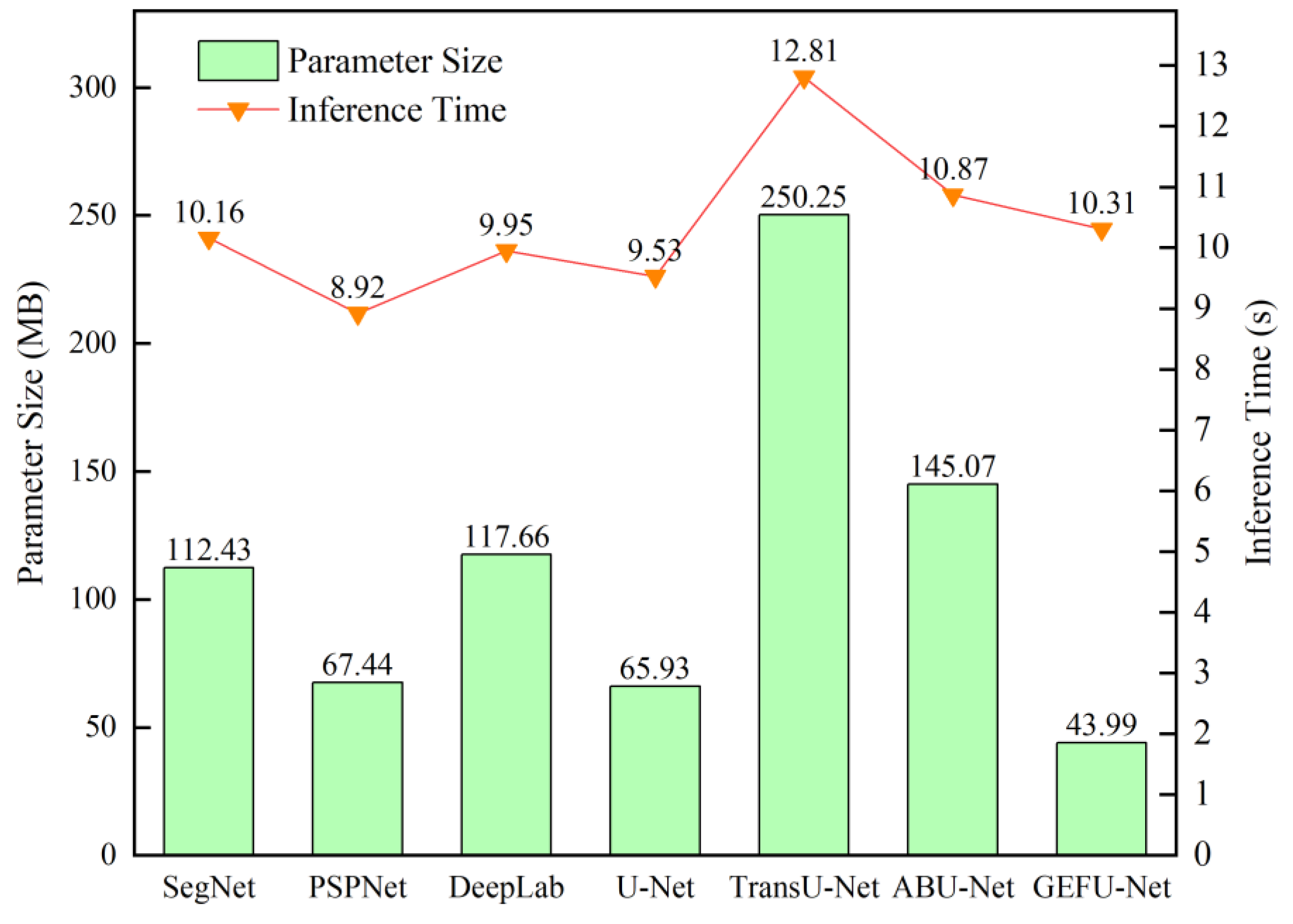
The proposed GEFU-Net is applied to a real Antarctic sea ice extraction scenes, and the analysis reveals that the proposed model achieves the best balance between the deployed parameter size and the inference speed.

The remainder of the paper is organized as follows. Section 2 outlines the pertinent aspects of the study data and details the specific methodologies employed in their processing. Section 3 offers an in-depth explanation of the proposed methodology, including the overall architecture of the model and the detailed configuration of each module. Section 4 describes the detailed experimental setup and a series of experimental results, which are briefly analyzed. Section 5 discusses the experimental results. Finally, Section 6 provides a comprehensive summary of the whole paper.

2. Materials

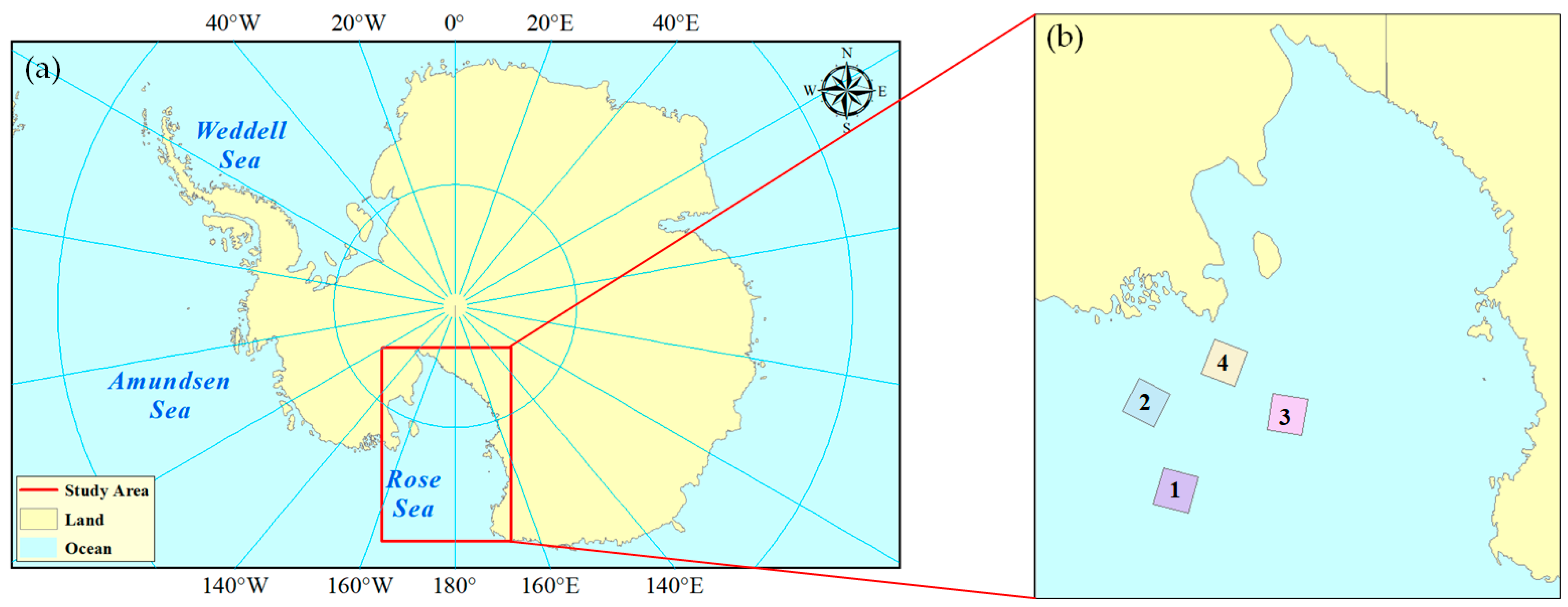
2.1. Study Area and Spectral Data Preparation

For this study, we choose the Ross Sea as our research area, due to its ecological importance and the wealth of available data; it has been the focus of numerous international scientific expeditions and research activities [30]. Specifically, the study area spans latitudes 70° to 78° S and longitudes 140° to 180° W. For clarity, the precise study area and the data parameters are presented in Figure 1a.

Figure 1. The area of interest for this study. (a) The red rectangles represent specific geographic areas. (b) The specific location of each scene.

The validity of the methodology was been assessed using the Sentinel-2 product. As an integral component of the European Union’s Copernicus Program, Sentinel-2 is primarily focused on the observation of the Earth’s surface and the monitoring of environmental conditions. These data are provided by the Copernicus data space ecosystem [6] in an open-access manner. As shown in Figure 1b, four scenes from October to December were selected, and detailed information on of the selected scenes is presented in Table 1. Sea ice with insufficient thickness may exhibit low contrast in remotely sensed images. Complex boundaries and fragmented distributions also make its extraction very challenging.

Table 1. Detailed information on the Sentinel-2 data for the Ross Sea.

ID	File Name	Date	Cloud (%)
1	S2B_MSIL1C_20181031T191509_N0500_R027_T03CXV	Oct 2018	0.05
2	S2B_MSIL1C_20191123T183459_N0500_R141_T05CMT	Nov 2019	0.00
3	S2B_MSIL1C_20201209T191509_N0500_R027_T02CNB	Dec 2020	0.00
4	S2B_MSIL1C_20231215T184459_N0510_R041_T04CDA	Dec 2023	1.06

TCI is a kind of imagery synthesized by three bands of red, green, and blue, which represent natural colors close those perceived by the human eye’s vision; this imagery is often used in multispectral remote sensing for environmental monitoring [31]. In Sentinel-2, the red, green, and blue bands correspond to 2, 3, and 4 bands, respectively; specific information on the bands is given in Table 2. As shown in Figure 2, after band synthesis, a linear stretching of 2% is applied to enhance the brightness and contrast of the image while removing outliers. Non-overlapping cropping is subsequently performed to generate a set of 512 × 512 samples. The mask image, obtained by annotating the cropped TCI samples, is used as the true value, while the corresponding TCI samples serve as the original input image.

Table 2. Detailed information on the spectral bands of the Sentinel-2B sensor.

Bands	Central Wavelength (nm)	Bandwidth (nm)	Spatial Resolution (nm)
Band 2—Blue	492.1	66	10
Band 3—Green	559.0	36	10
Band 4—Red	664.9	31	10

Figure 2. A schematic diagram of the Sentinel-2 data preprocessing.

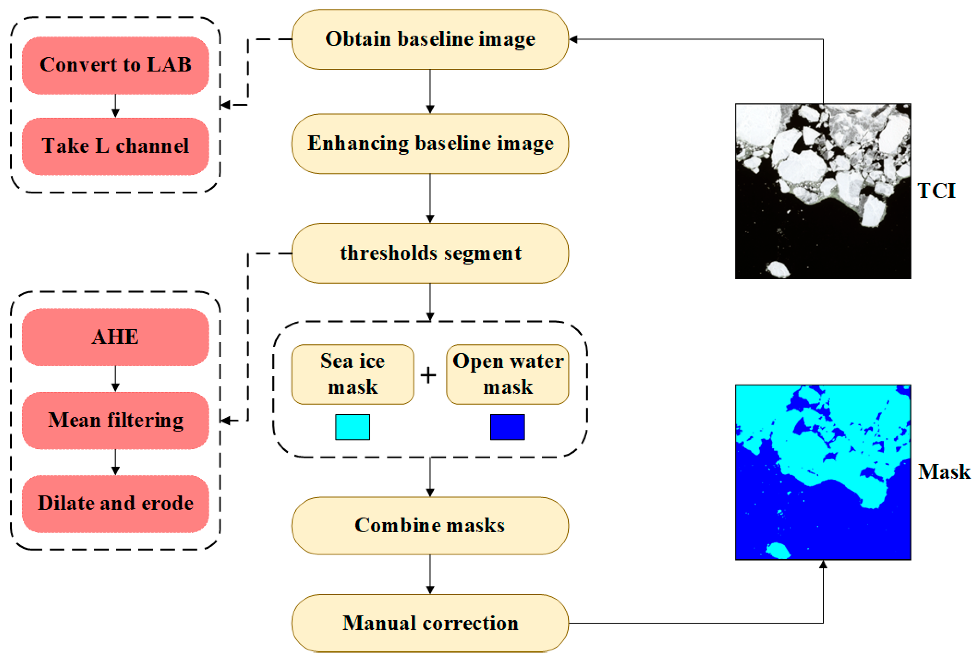
2.2. Production Process of Dataset

In this study, the images were annotated according to two categories: sea ice and open water. However, accurate annotating of high-resolution remotely sensed images is challenging, and it is noted that scientists often annotate sea ice images based on optical properties [32]. Thick sea ice appears white or grayish-white. Thin ice may exhibit some transparency and cyan cracks, and open water is generally dark black. Inspired by [32], a simple image processing method was employed to assist in the annotation of sea ice.

The specific process of sea ice annotation is shown in Figure 3. In the first step, TCI is converted to LAB color space, and the L channel is extracted as the baseline image for annotation. In the second step, the image enhancement technique is selected based on the scene in the remote sensing image, and the specific image enhancement process includes the following: enhancing the contrast between thin ice and open water using adaptive histogram equalization (AHE); eliminating the edge effect caused by AHE using mean filtering; and reinforcing the edge features of the sea ice through operations such as image expansion and erosion. It should be noted that these operations strengthen the continuity of the sea ice, but may weaken its individuality, e.g., eliminating small gaps between ice cubes. In the third step, most of the sea ice is annotated by manually setting a suitable threshold. Finally, the mask image is obtained through manual correction and supplementation.

Figure 3. A schematic diagram of the sea ice annotation.

Using the above methodology, a total of 1764 samples were generated. Furthermore, to evaluate the proposed model, 70% of the data was randomly selected for training, and 30% for testing, for each ID.

3. Methods

3.1. Overview

The specific flow chart of the proposed Antarctic sea ice extraction method is shown in Figure 4. After preprocessing the Sentinel-2 data, some Antarctic sea ice TCI samples are obtained. The TCI samples are annotated to obtain masks, and the samples and corresponding masks are divided into a training set and a test set. The data in the training set are fed into the GEFU-Net model for training, and the extraction effect is quantitatively evaluated using the test set data and various evaluation metrics to retain the optimal model parameters. Finally, the model, loaded with optimal parameters, achieves accurate extraction of sea ice. It is worth noting that in GEFU-Net, the down-sampling operation in the encoder’s residual blocks is improved to make full use of the available information in the feature extraction process. Meanwhile, the SEGR module performs graph reconstruction on the deep features extracted by the encoder and constructs the adjacency matrix quickly and efficiently using GAAST, which effectively improves the extraction accuracy of the sea ice model by supplementing and enhancing the semantic information in the features through aggregation of pixel nodes.

Figure 4. A flowchart of sea ice extraction using Sentinel-2 data in our scheme.

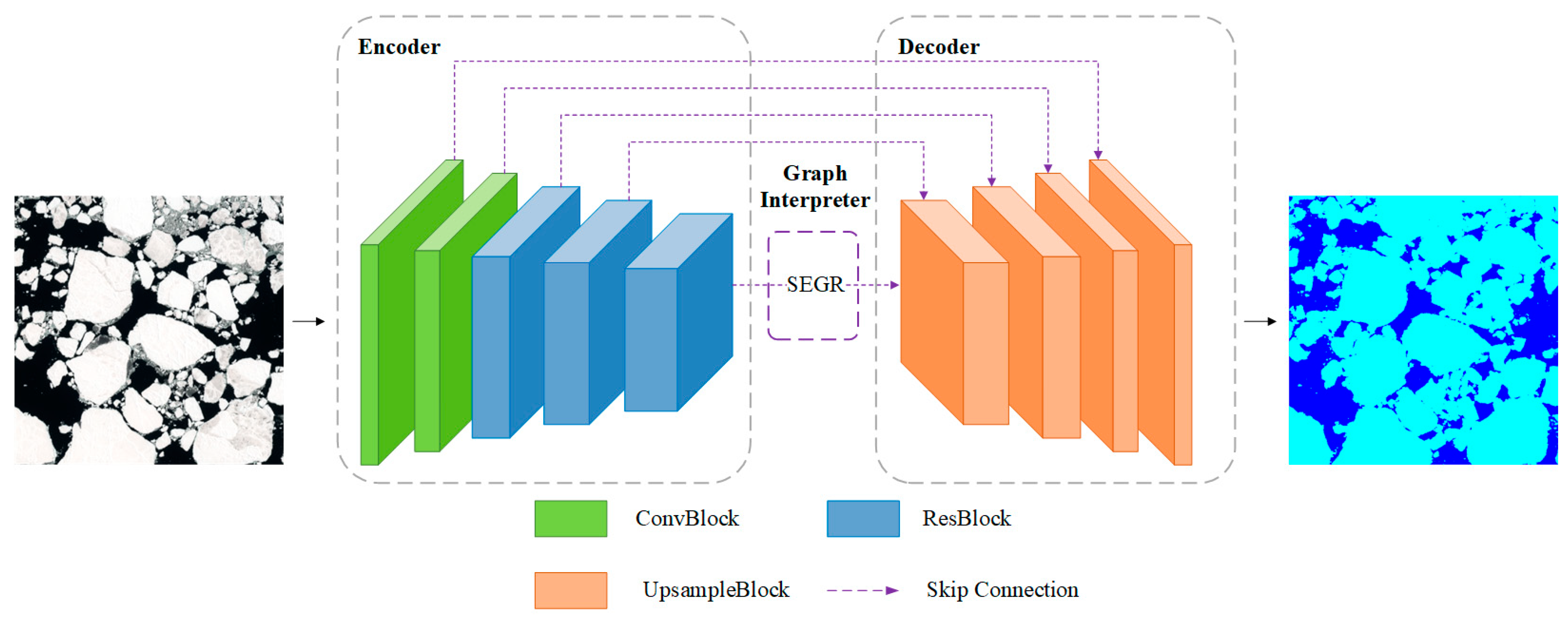
3.2. Overall Structure of GEFU-Net

The overall structure of GEFU-Net is shown in Figure 5. It consists of three parts: an encoder, a graph interpreter, and a decoder. The encoder is primarily composed of ConvBlocks and ResBlocks, which facilitate the extraction of deep feature maps from shallow to deep levels. The graph interpreter is the SEGR module, which improves the accuracy of sea ice extraction by enhancing and supplementing semantic information with graph reconstruction of features. The decoder is composed of UpsampleBlocks, which gradually revert the feature to its original size, and the final extraction result is output using a convolution operation with a kernel size of 1 × 1.

Figure 5. The overall structure of the proposed GEFU-Net.

3.2.1. Backbone Network of Encoder

The encoder backbone structure is shown in Figure 6. The ConvBlocks are responsible for extracting shallow features, and primarily consist of convolution operations. ResBlocks are responsible for extracting deep features, inspired by ResNet [33], and consist of a convolution branch and a residual branch. In the convolution branch, the down-sampling operation is performed by 3 × 3 convolution, and the channel alignment operation is performed by 1 × 1 convolution. In the residual branch, to make full use of the original feature information, the 1 × 1 convolution used for down-sampling is replaced by 2 × 2 average pooling, and the 1 × 1 convolution is used solely for channel alignment. Details of the different down-sampling operations are shown in Figure 7. After inputting TCI, the feature $X_i(i =1, 2, 3, 4, 5)$ can be obtained by the encoder, from shallow to deep layers and from large to small resolutions.

Figure 6. A schematic diagram of the encoder, consisting of ResBlocks and ConvBlocks.

Figure 7. Different down-sampling operations in the residual branch. (a) Convolution, (b) average pool.

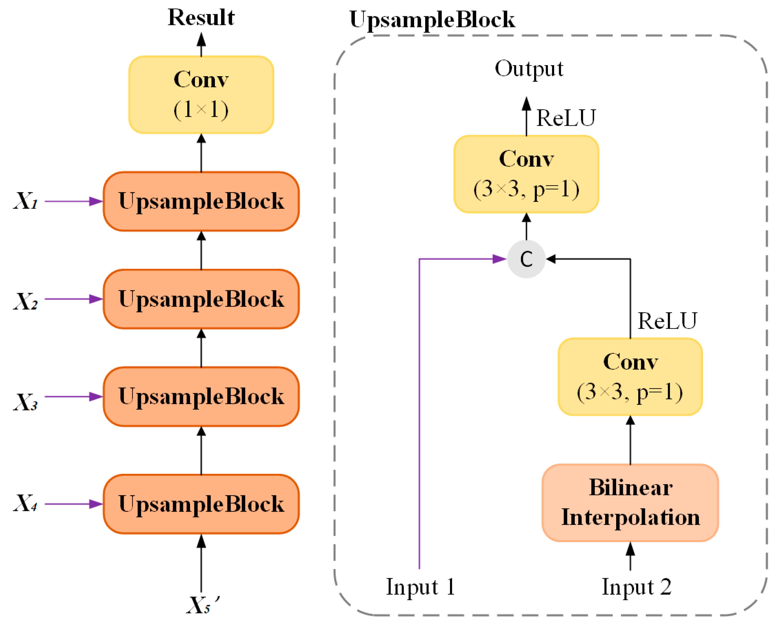
3.2.2. Backbone Network of Decoder

The decoder backbone structure is shown in Figure 8. Each UpsampleBlock performs a step-by-step recovery of the features to their original size, and ultimately completes the output of the result through a convolution operation. The bilinear interpolation operation doubles the feature size, while the convolution operation completes the channel alignment. In addition, skip connections and convolution operations are used to further complete the fusion of features. Finally, the result is output through a convolution operation with a kernel size of 1 × 1.

Figure 8. A schematic diagram of the decoder, consisting of UpsampleBlocks.

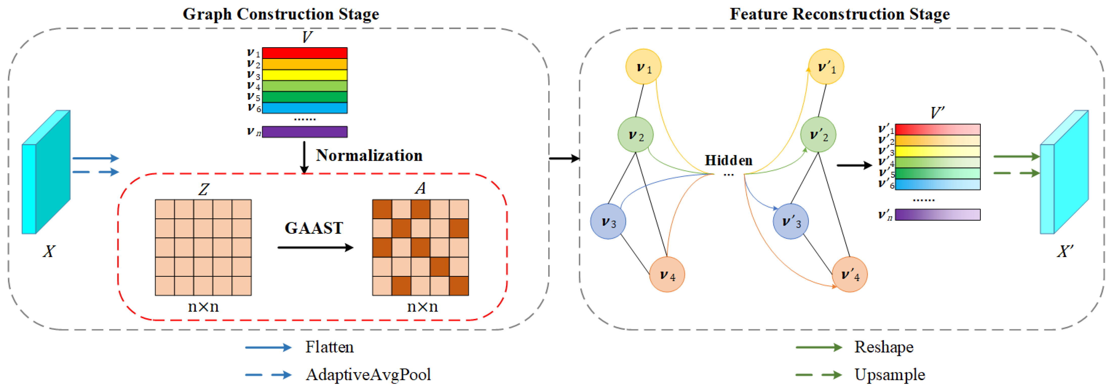
3.2.3. SEGR Module of Graph Interpreter

In the encoder, the shallow features extracted by the convolution blocks typically contain low-level information, such as edges and textures. The deep features extracted by the residual block usually contain abstract global features, but many of them are often invalid and redundant due to a lack of detailed semantic information, such as context. However, this information is necessary for the accurate identification of sea ice, including thin ice and broken ice. To address the lack of high-level semantic information, such as context, in traditional convolutional deep features, a novel module, SEGR, is introduced. This module supplements the input deep features with high-level semantic information through graph reconstruction.

The specific structure of SEGR is shown in Figure 9. A feature $X\in R^{C\times H\times W}$ is assumed to be extracted by the encode. The goal of SEGR is to transform the input feature into graph-structured data, and complete the fusion of each node through a GCN to capture the interdependencies between pixels and obtain the reconstructed features. SEGR consists of two main stages: the graph construction stage and the feature reconstruction stage.

Figure 9. A schematic diagram of the SEGR module.

In the graph construction stage, the number of nodes N = H × W depends on the size of the input feature graph. If N is too large, it will require more computational resources. Therefore, for larger feature graphs, a parameter-free adaptive average pooling operation is used to compress the feature graph and limit its size. Afterward, a flattening operation is applied to obtain the node features $V {\in R}^{N\times C}$. This is expressed by the following formula:

$$V=Flatten[AdaptiveAvgPool(X)]$$

(1)

When constructing the adjacency matrix, common methods include selecting k nearest neighbors based on distance metrics [34], including Euclidean distance and Manhattan distance. This requires an appropriate choice of distance metric and a specific value of k, which limits the general applicability of these methods. For instance, in a high-dimensional space, calculating the distances between nodes not only increases computational cost, but may also render the results invalid [35]. It is believed that the dot product of vectors is not only effective in reflecting the similarity between vectors, but also has a smaller computational cost and is more easily implemented [25]. Therefore, the GAAST is designed for constructing the adjacency matrix. To mitigate the influence of the size of the node’s features, each feature is normalized, and the similarity matrix $Z {\in R}^{N\times N}$ is obtained through the dot product of $V$ and $V^T$. A threshold is then constructed based on the global average similarity, to determine the adjacency relationship between the nodes. This is expressed by the following formulas:

$$Z=Norm(V)·Norm(V^T)$$

(2)

$$A_{ij}=\left\{\begin{array}{cc}1,& Z_{ij}\ge \alpha ·mean(Z),i\ne j\\ 0,& else\end{array}\right.$$

(3)

where $A_{ij}(i,j\in 1,2,3\dots N)$ denotes the adjacency between the ith node and the jth node, and $\alpha$ is a trainable weight parameter with an initial value of 1, which is used to determine the optimal adjacency matrix construction scheme automatically through training optimization of the data. The above operation provides the graph representation $G (V, A)$ of X. It is worth noting that A is a symmetric matrix.

In the feature reconstruction stage, the adjacency matrix A obtained from the above equation contains only information about the adjacency relationships between nodes, while disregarding information about the nodes themselves. Moreover, due to the lack of normalization in the adjacency matrix, the value of similarity between some nodes may become excessively large. Therefore, the following operation is applied to all the provided graphs $G (V, A)$ before graph convolution:

$$\widehat{D}=diag({\widehat{d}}_1,{\widehat{d}}_2,{\widehat{d}}_3,\dots ,{\widehat{d}}_N)$$

(4)

$${\widehat{d}}_i={\displaystyle \sum _j{(A+I)}_{ij}}$$

(5)

$$\widehat{A}={\widehat{D}}^{-\frac{1}{2}}(A+I){\widehat{D}}^{-\frac{1}{2}}$$

(6)

where $I$ is unit matrix and $\widehat{D}$ is the degree matrix of $A+I$. The formula for updating the node state in GCN is defined as follows:

$$V^{(l+1)}=\sigma (\widehat{A}{V}^{(l)}{w}^{(l)})$$

(7)

where $l$ represents the lth layer, w is learnable weight parameter, and $\sigma (·)$ is activation function.

The updated graph node feature $V^{\prime }$ is obtained through the above operation. The reconstructed feature $X^{\prime }$ is obtained by a reshaping operation. If the features are pooled, they are restored to the size of input feature graph X using a parameter-free bilinear interpolation up-sampling operation.

$$X\prime =Upsample\left[Reshape\right(V\prime \left)\right]$$

(8)

3.3. Loss Function

In this paper, focal loss [36] is chosen as the loss function for model training. It addresses the model performance issue caused by data imbalance. The approach adaptively adjusts the contribution of each sample to the loss based on the prediction accuracy, by introducing coefficient factors on top of cross-entropy loss. This helps to attenuate the learning of easy samples and enhance the learning of difficult samples, thereby improving the model’s classification ability. The specific definition of $L_{\mathit{Focal}}$ is as follows:

$$L_{Focal}=-{\displaystyle \frac{1}{N}}{\displaystyle \sum _{i=1}^N\left[\alpha {(1-p_i)}^{\gamma }{y}_i\log \right(p_i)+(1-\alpha \left){p_i}^{\gamma }\right(1-y_i\left)\log \right(1-p_i\left)\right]}$$

(9)

where α is used to address the problem of sample size imbalance, and γ is used to regulate the impact of the difference between the prediction results and the true values on the loss.

4. Results

4.1. Experimental Platform and Parameter Setting

The dataset produced in Section 2 was used to test the performance of the proposed model and compare it with several models from recent years in the field of sea ice segmentation in spectral remote sensing images, including DeepLabV3+ [37], PSPNet [16], and SegNet [16]. In particular, U-Net with an attention block (ABU-Net) [38] and TransU-Net [39], which share similar concepts with our approach, are also included for comparison. All experiments were conducted on a personal computer with an Intel Core i9-13900K CPU, an NVIDIA GeForce RTX 4090 GPU, and 128 GB of RAM. The semi-automatic annotation of sea ice was implemented using the OpenCV 4.10.0. All models were built using the PyTorch 2.0.1 deep learning framework.

To ensure the reliability of the experimental results, the hyperparameters for model training were configured uniformly, as shown in Table 3. Most of the training hyperparameters were adapted from existing research [37], including learning rate, optimizer, and loss function parameters [36]. The batch size was set to 8, and the number of epochs was set to 200. None of the models used pretrained weights; instead, a uniform initialization method was applied. Additionally, no enhancement techniques were used during training.

Table 3. Hyperparameter configuration of network training.

Parameters	Values	Parameters	Values
Optimizer	Adam	Size limitation of SEGR	32 × 32
Learning rate	$1 \times {10}^{-4}$	GCN layers	2
Epoch	200	γ	2
Batch size	8	α	0.3

4.2. Evaluation Metrics

The extraction of sea ice from TCI can be considered analogous to the semantic segmentation task in computer vision. Therefore, relevant evaluation metrics from semantic segmentation tasks were used to comprehensively evaluate the extraction results of the different models in the experiment.

Pixel accuracy (PA), Intersection over Union (IoU), and F1-Score will be used for the quantitative analysis of the results from different sea ice extraction methods. All evaluation metrics can be derived from the confusion matrix. TP represents the number of pixels that correctly predict sea ice, FP represents the number of pixels that incorrectly predict open water as sea ice, TN represents the number of pixels that correctly predict open water, and FN represents the number of pixels that incorrectly predict sea ice as open water. The defining equations for these metrics are as follows:

$$PA={\displaystyle \frac{TP+TN}{TP+TN+FP+FN}}$$

(10)

$$IoU={\displaystyle \frac{TP+TN}{TP+FP+FN}}$$

(11)

$$Precision={\displaystyle \frac{TP}{TP+FP}}$$

(12)

$$Recall={\displaystyle \frac{TP}{TP+FN}}$$

(13)

$$F1\text{-}Score=2\times {\displaystyle \frac{Precision\times Recall}{Precision+Recall}}$$

(14)

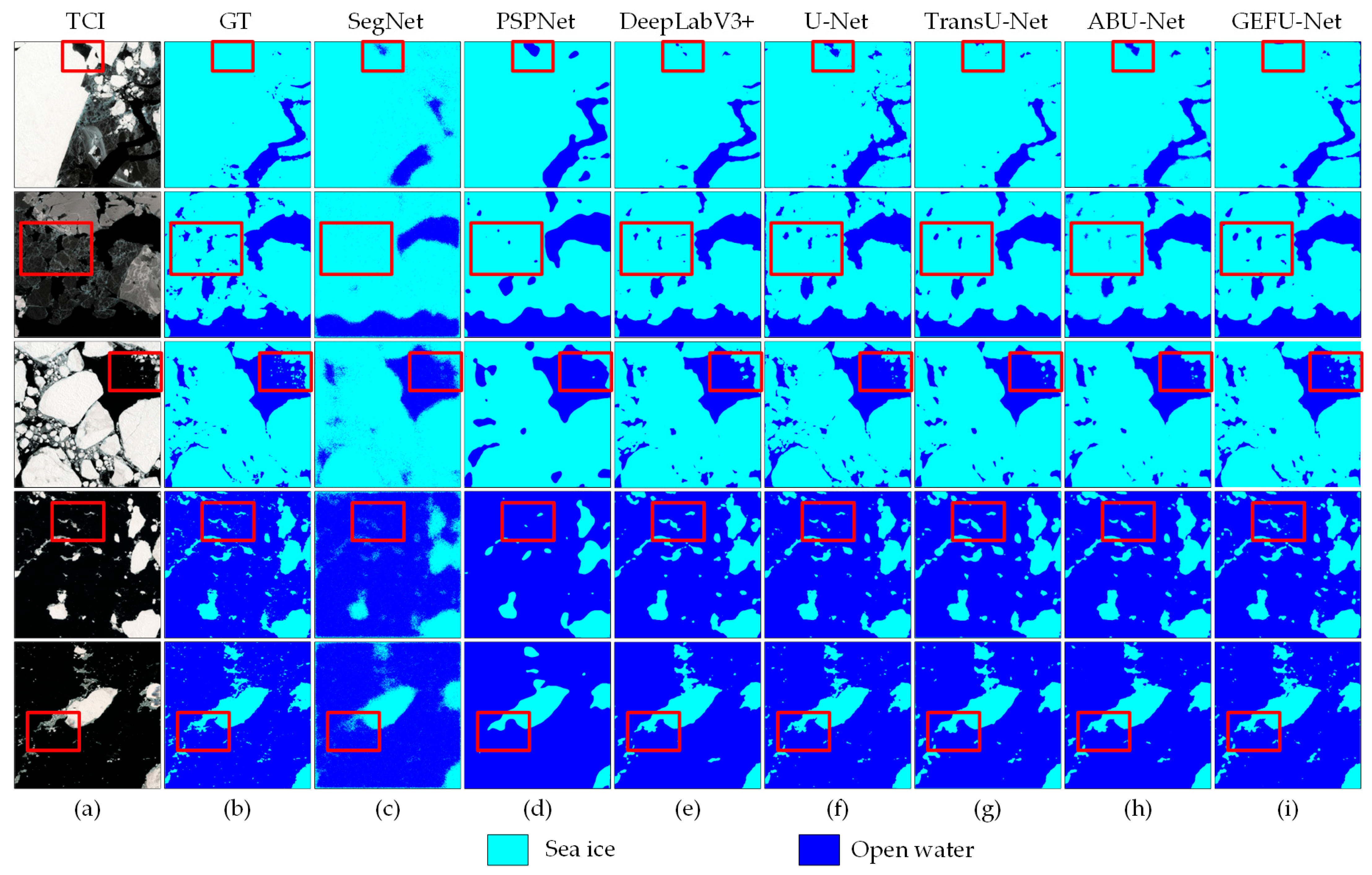
4.3. Ice Extraction Results

To verify the effectiveness of different models in sea ice extraction, some data from the test set were selected for display. The final extraction results of the selected TCI and different models are shown in Figure 10, where light blue represents sea ice and dark blue represents open water. The feature extraction backbone network used in other models is ResNet18, and the residual block selected in DeepLabV3+ is a bottleneck block, which is adapted to the ASPP module.

Figure 10. Sea ice extraction results from different models. (a) TCI, (b) ground truth, (c) SegNet, (d) PSPNet, (e) DeepLab, (f) U-Net, (g) TransU-Net, (h) ABU-Net, (i) GEFU-Net.

As shown in Figure 10c, SegNet uses the ensemble index saved at the encoding stage for up-sampling during the decoding process. Although this method preserves spatial information, the up-sampling process may lead to the loss of some fine feature details, resulting in blurred recognition of sea ice and open water edges. In Figure 10d, PSPNet effectively extracts multiscale features through the pyramid pooling module, which improves recognition accuracy to some extent. However, the fusion process of multiscale features may cause the features of small targets to become diluted. In Figure 10e,f, DeepLabV3+ uses inflationary convolution to expand the receptive field and obtain contextual information in the features. This method provides better segmentation results than SegNet and PSPNet, but still faces challenges in recognizing irregular boundaries and small targets. U-Net achieves good segmentation results for small targets with complex shapes through its layer-by-layer sampling structure. However, its underlying features lack sufficient global information, which may result in the misclassification of thin ice as open water, and limited segmentation effectiveness in complex scenes such as melting pools in thin ice. In Figure 10g,h, TransU-Net adopts a similar improvement approach and enhances the ability to extract smaller targets. However, it also has the potential to over-extract. ABU-Net, which introduces an attention mechanism, can effectively recognize complex environments such as fine ice and melt ponds through multilevel fusion reconstruction of extracted features. In contrast, the proposed GEFU-Net not only effectively identifies the details of thin ice and sea ice edges, but also demonstrates excellent segmentation performance for fine ice fragments and ice melt pools, as shown in Figure 10i.

As shown in Table 4, we quantify the extraction results of different methods based on three metrics: PA, IoU, and F1-Score. It is observed that deep learning methods significantly outperform the traditional image segmentation method, Otsu. Furthermore, among the deep learning models, GEFU-Net shows improvements of 0.52%, 0.98%, and 0.51% in PA, IoU, and F1-Score, respectively, compared to U-Net. All metrics of GEFU-Net surpass those of other models, providing compelling evidence of its efficacy.

Table 4. Comparison of evaluation metrics of sea ice extraction results from different models.

	Method	PA (%)	IoU (%)	F1-Score (%)
Traditional Technology	Otsu	81.43	66.59	79.94
Deep Learning Model	SegNet	91.79	86.52	92.78
	PSPNet	94.72	90.75	95.15
	DeepLabV3+	97.01	94.79	97.32
	U-Net	97.00	94.68	97.27
	TransU-Net	96.45	93.92	96.86
	ABU-Net	96.99	94.75	97.31
	GEFU-Net	97.52	95.66	97.78

4.4. SEGR Module Analysis

4.4.1. Effect of SEGR Module Location and Number on the Extraction Results

To verify the effectiveness of the SEGR module in the proposed model, ablation experiments were conducted based on the above example by placing SEGR at different block levels. The shallow features extracted by the convolution blocks are denoted as $X_1, X_2$, and the deep features extracted by the residual blocks are denoted as $X_3, X_4, X_5$. The specific experimental results are shown in Table 5. Case 1 represents the baseline network and Case 1 represents the baseline network, while Cases 2 to 6 illustrate the effect of the SEGR module on graph reconstruction with a single level of features. It is evident that graph reconstruction of deeper features improves the overall performance of the model, highlighting the significance of unstructured information in deep features for sea ice identification. Additionally, the global information in deep features can be further enhanced through graph reconstruction. Cases 7 to 10 demonstrate the effect of graph reconstruction on multiple levels of deep features using the SEGR module. It is evident that graph reconstruction of multilevel features degrades the model’s performance, with the degradation being more pronounced when the reconstructed features are from similar levels. A primary reason is that the GCN tends to homogenize individual pixel features, making the overall features smoother. When two feature levels are close, the overall feature distribution of the pixels in the deeper features after graph reconstruction and up-sampling is more similar than that of the shallower features after graph reconstruction.

Table 5. The effects of SEGR module location and number on the results of the model’s extraction.

	${\mathit{X}}_1$	${\mathit{X}}_2$	${\mathit{X}}_3$	${\mathit{X}}_4$	${\mathit{X}}_5$	PA (%)	IoU (%)	F1-Score (%)
Case 1						96.63	94.10	96.96
Case 2	$\surd$					97.39	95.42	97.66
Case 3		$\surd$				97.10	94.85	97.36
Case 4			$\surd$			96.68	94.13	96.97
Case 5				$\surd$		97.39	95.36	97.62
Case 6					$\surd$	97.52	95.66	97.78
Case 7			$\surd$		$\surd$	96.84	94.46	97.15
Case 8				$\surd$	$\surd$	96.60	93.94	96.87
Case 9			$\surd$	$\surd$		96.06	93.19	96.48
Case 10			$\surd$	$\surd$	$\surd$	85.40	73.79	84.91

4.4.2. Effect of GAAST on Adjacency Matrix Generation

In the SEGR module, the adjacency matrix was constructed using the GAAST. To illustrate the superiority of this method, comparisons were made with commonly used distance metrics, including Euclidean distance and Manhattan distance. As shown in Figure 11, the parameter k denotes the number of neighbors for each node, with k = 0 representing the GAAST.

Figure 11. Comparison of different adjacency matrix generation methods. (a) Euclidean distance. (b) Manhattan distance.

As shown in Figure 11a,b, the left side of the coordinates indicates the inference time for each sample, while the right side indicates the pixel accuracy of the extraction. It is observed that the inference time for both distance metrics increases with k, and an optimal k exists to achieve the best extraction results. Compared with distance metrics, the proposed GAAST does not require manual parameter setting. The dot product operation effectively improves conversion efficiency, allowing the SEGR module to achieve a shorter inference time while maintaining good reconstruction results. Considering that a scene consists of hundreds of samples, the GAAST will significantly enhance the sea ice extraction efficiency of GEFU-Net.

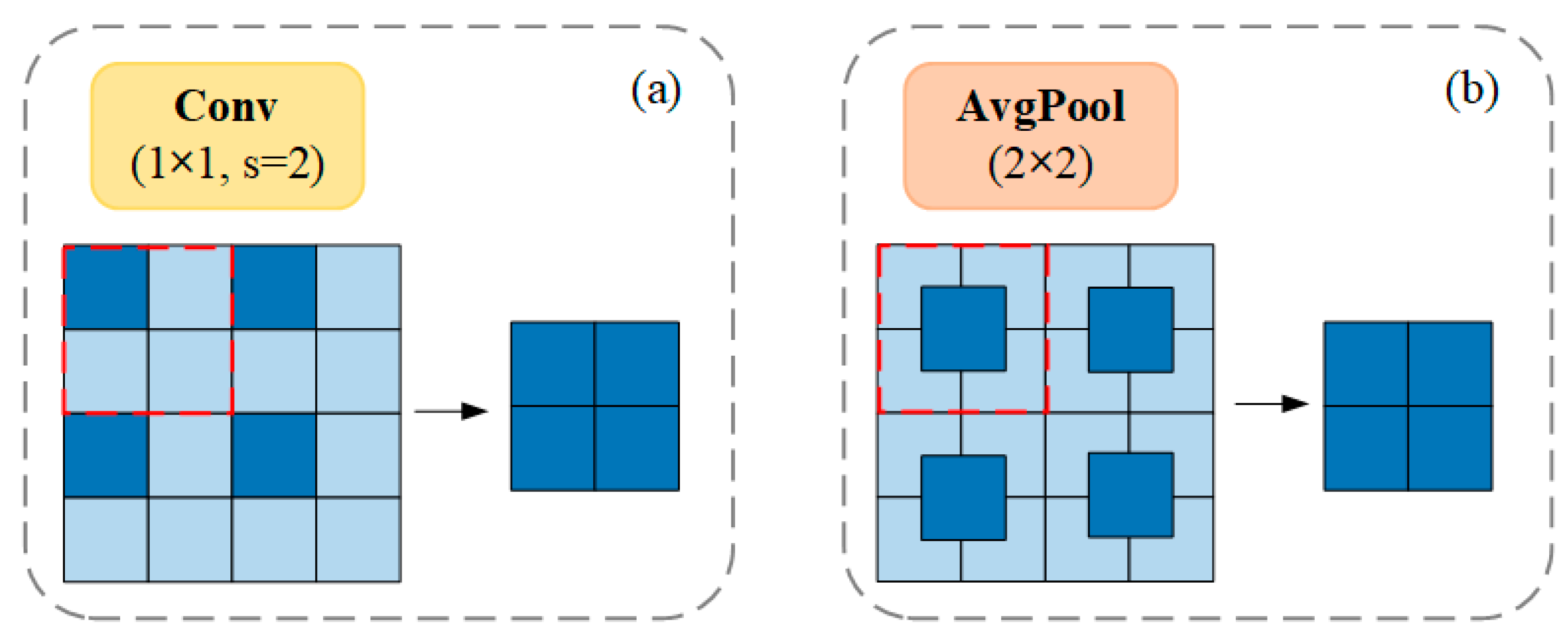
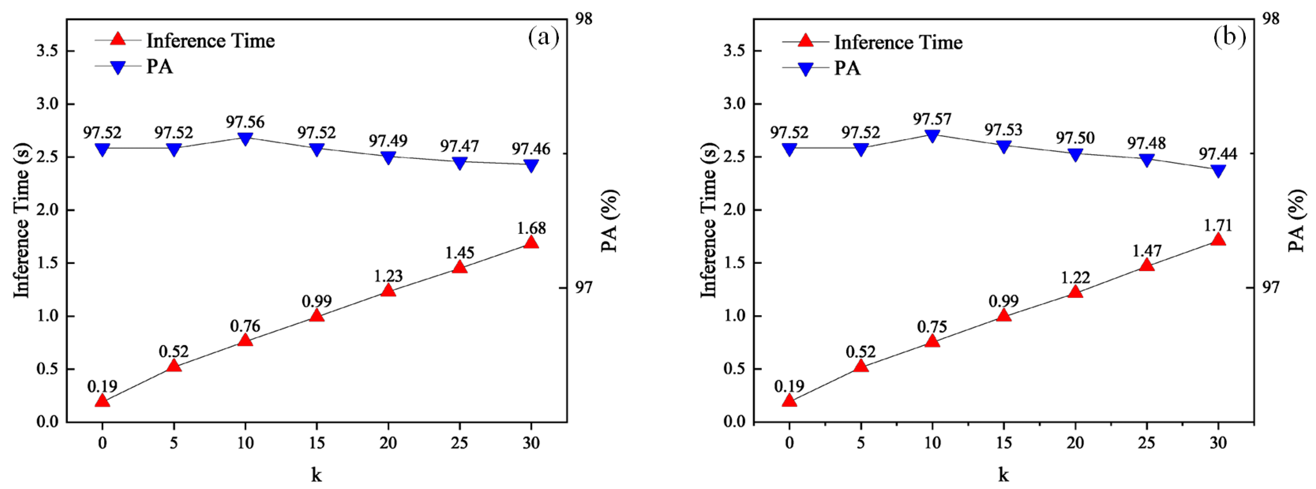
4.4.3. Effect of Adaptive Pooling Size on Extraction Results in SEGR

In the SEGR module, a global average pooling operation was applied to limit the number of feature nodes by reducing the size of the features. To investigate the effect of the pooling operation on the extraction results, extraction metrics under different pooling sizes were analyzed. As shown in Table 6, a decreasing trend in extraction performance is observed as the feature size is reduced. This is because the pooling operation compresses the features, reducing their dimensions and potentially leading to a loss of detailed information.

Table 6. The effects of different pooling sizes in the SEGR module on the extraction results.

Feature Size Limitation	PA (%)	IoU (%)	F1-Score (%)
32 × 32	97.52	95.66	97.78
16 × 16	96.68	94.10	96.96
8 × 8	96.70	94.12	96.97
4 × 4	96.68	94.10	96.96
2 × 2	96.66	94.07	96.94

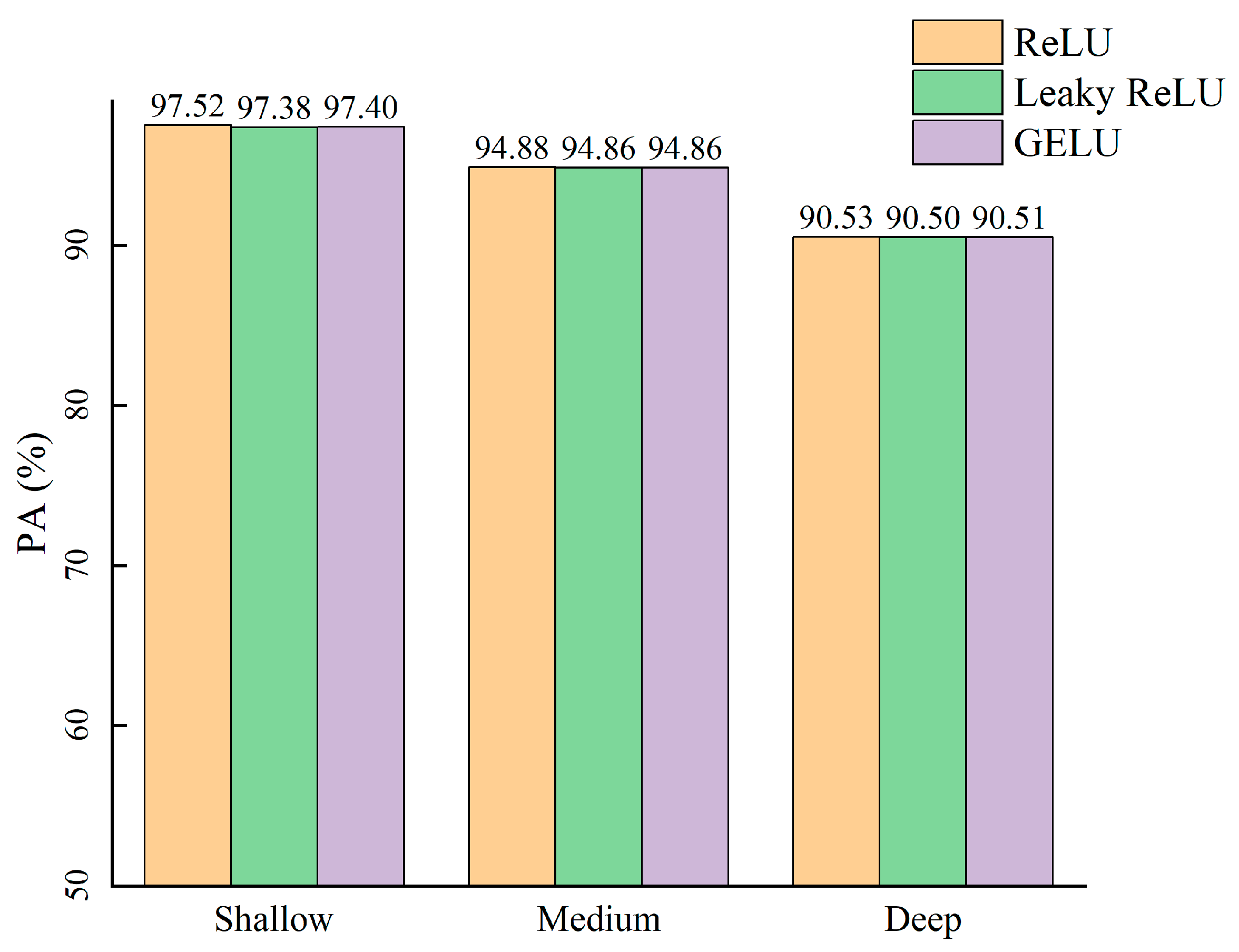
4.4.4. Effect of Number of GCN Layers on Extraction Results in SEGR

The GCN consists of a simple MLP, which captures dependencies between nodes at greater distances as the number of layers increases. However, an increase in layers may cause fused node features to become oversmoothed, leading to performance degradation. To investigate the effect of the number of GCN layers on the performance of the feature reconstruction phase in the SEGR module, comparative experiments were conducted on shallow, medium, and deep GCN layers, with specific parameter configurations shown in Table 7. C denotes the number of input node features. In addition, extraction metrics under common activation functions in the MLP were also analyzed, with the results presented in Figure 12.

Table 7. Specific configurations for different GCN layers.

Type	GCN Layers	Channels	Bias	Drop
Shallow	2	C-C/2-C	False	0.1
Medium	4	C-C/2-C/4-C/2-C	False	0.1
Deep	6	C-C/2-C/4-C/8-C/4-C/2-C	False	0.1

Figure 12. Effect of GCN layers in SEGR module on extraction results.

The experimental results show that the shallow GCN achieves better performance in sea ice extraction. Meanwhile, the comparison indicates that the activation function of the MLP has less influence in SEGR, with ReLU demonstrating a slight advantage overall, possibly due to the low complexity of the sea ice extraction task in this study.

5. Discussion

5.1. Limitations of SEGR Module

It should also be noted that the SEGR module proposed in this study has certain limitations. When constructing the adjacency matrix using GAAST, the importance of each node’s adjacent relationship is treated equally, with values of 0 or 1, which does not emphasize the varying importance of adjacent relationships between a node and different nodes. In addition, the converted graph structure is undirected, ignoring spatial information between nodes, which may be crucial for the fusion of pixel node features.

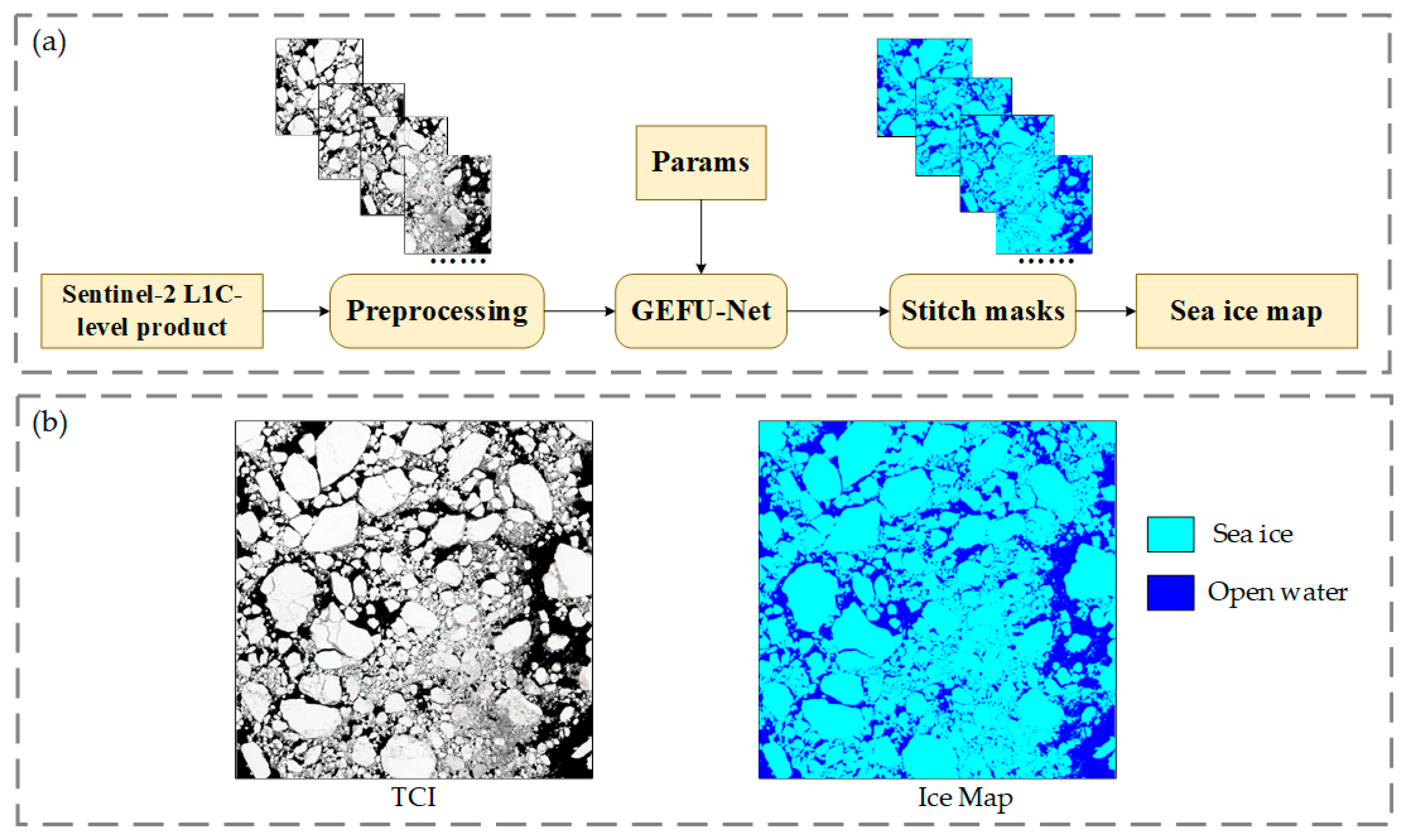
5.2. Application of Sea Ice Mapping in Remote Imaging

Compared to manual ice mapping by experts, automatic ice mapping using deep learning techniques offers significant advantages in terms of mapping efficiency, data compatibility, and cost-effectiveness, especially in large-scale, continuous monitoring scenarios [40]. To demonstrate the feasibility of the proposed model in automatic ice mapping applications, the trained GEFU-Net model was applied to the entire Sentinel-2 dataset.

The exact process of automated ice mapping is shown in Figure 13a. First, the obtained Sentinel-2 data are preprocessed to generate a certain number of TCI samples. Second, sea ice extraction is performed on each sample using GEFU-Net to obtain a sea ice mask. Finally, the masks are sequentially stitched to create a complete ice map. This process is demonstrated using a Sentinel-2 product acquired in the Ross Sea on 15 December 2023, which is not included in our dataset. The specific extraction results are shown in Figure 13b. Subjectively, GEFU-Net not only effectively captures a wide range of sea ice, but also accurately extracts thin and fine ice. The extraction results were manually objectively evaluated, and were found to achieve an accuracy of 96.91%, indicating the strong applicability of the proposed model.

Figure 13. GEFU-Net applied for automatic ice mapping using Sentinel-2 data. (a) Flowchart of ice mapping. (b) Ice mapping results—dark blue for open water, light blue for sea ice.

In addition, the size of the model’s parameters significantly impacts memory consumption, hardware requirements, and energy costs during actual deployment. The number of parameters deployed and the inference time for different models were calculated during the ice mapping process described above.

As shown in Figure 14, among several mainstream segmentation models, U-Net not only achieves better sea ice extraction results, but also has fewer model parameters, making it widely used in ice mapping applications [41]. Although TransU-Net and ABU-Net improve the accuracy of the models by improving U-Net, they introduce huge model parameters, which complicates actual deployment. In contrast, the proposed GEFU-Net achieves the best performance with a parameter size of only 43.99 MB, 33.28% smaller than that of U-Net, and an inference time of 10.31 s, only 8.18% longer than that of U-Net. This is due to the use of the GAAST for graph structure conversion in the SEGR module, which effectively enhances conversion efficiency. Additionally, the GCN uses a simple MLP for feature reconstruction, reducing the introduction of additional parameters. Combined with efficient data transfer techniques and model compression methods such as quantization, pruning, and distillation, GEFU-Net offers an effective solution for real-time automated ice mapping.

Figure 14. Parameter size and inference time of different models.

6. Conclusions

This paper briefly analyzes the current research on polar sea ice extraction using remote sensing images and deep learning techniques. A deep learning model, GEFU-Net, is proposed for the accurate extraction of Antarctic sea ice. GEFU-Net is constructed based on the U-Net architecture and GNNs. Through a series of experiments, the SEGR module is introduced, which significantly improves sea ice extraction accuracy by graphically reconstructing the deep features obtained from the encoder. In transforming the input features into graph-structured data, the GAAST is proposed for constructing the adjacency matrix, effectively enhancing conversion efficiency while maintaining high-quality extraction results. In the practical application of ice mapping, Sentinel-2 data were chosen for validation. The results demonstrate that GEFU-Net has the fewest model parameters and satisfactory inference speed compared to other models, providing an effective solution for automated sea ice extraction.

In future work, to fully exploit the versatility of the SEGR module for image features, it will be integrated into more established CNN frameworks in remote sensing to further improve the efficiency and accuracy of the model for sea ice extraction. Additionally, cloud cover inevitably affects multispectral remote sensing imaging, which can significantly impact sea ice extraction results. Therefore, combining data from other remote sensing sources for sea ice extraction presents a promising research direction.

References

- Eayrs, C.; Li, X.; Raphael, M.N.; Holland, D.M. Rapid decline in Antarctic sea ice in recent years hints at future change. Nat. Geosci. 2021, 14, 460–464. [Google Scholar] [CrossRef]
- Purich, A.; Doddridge, E.W. Record low Antarctic sea ice coverage indicates a new sea ice state. Commun. Earth Environ. 2023, 4, 314. [Google Scholar] [CrossRef]
- Swadling, K.M.; Constable, A.J.; Fraser, A.D.; Massom, R.A.; Borup, M.D.; Ghigliotti, L.; Granata, A.; Guglielmo, L.; Johnston, N.M.; Kawaguchi, S. Biological responses to change in Antarctic sea ice habitats. Front. Ecol. Evol. 2023, 10, 1073823. [Google Scholar] [CrossRef]
- DeConto, R.M.; Pollard, D.; Alley, R.B.; Velicogna, I.; Gasson, E.; Gomez, N.; Sadai, S.; Condron, A.; Gilford, D.M.; Ashe, E.L. The Paris Climate Agreement and future sea-level rise from Antarctic. Nature 2021, 593, 83–89. [Google Scholar] [CrossRef] [PubMed]
- Zhang, X.; Deser, C. Tropical and Antarctic sea ice impacts of observed Southern Ocean warming and cooling trends since 1949. npj Clim. Atmos. Sci. 2024, 7, 197. [Google Scholar] [CrossRef]
- Yan, Q.; Huang, W. Sea ice remote sensing using GNSS-R: A review. Remote Sens. 2019, 11, 2565. [Google Scholar] [CrossRef]
- Han, Y.; Liu, Y.; Hong, Z.; Zhang, Y.; Yang, S.; Wang, J. Sea ice image classification based on heterogeneous data fusion and deep learning. Remote Sens. 2021, 13, 592. [Google Scholar] [CrossRef]
- Qiu, H.; Gong, Z.; Mou, K.; Hu, J.; Ke, Y.; Zhou, D. Automatic and accurate extraction of sea ice in the turbid waters of the yellow river estuary based on image spectral and spatial information. Remote Sens. 2022, 14, 927. [Google Scholar] [CrossRef]
- Cáceres, A.; Schwarz, E.; Aldenhoff, W. Landsat-8 Sea Ice Classification Using Deep Neural Networks. Remote Sens. 2022, 14, 1975. [Google Scholar] [CrossRef]
- Waga, H.; Eicken, H.; Light, B.; Fukamachi, Y. A neural network-based method for satellite-based mapping of sediment-laden sea ice in the Arctic. Remote Sens. Environ. 2022, 270, 112861. [Google Scholar] [CrossRef]
- Guo, W.; Itkin, P.; Singha, S.; Doulgeris, A.P.; Johansson, M.; Spreen, G. Sea ice classification of TerraSAR-X ScanSAR images for the MOSAiC expedition incorporating per-class incidence angle dependency of image texture. Cryosphere 2023, 17, 1279–1297. [Google Scholar] [CrossRef]
- Chen, S.; Yan, Y.; Ren, J.; Hwang, B.; Marshall, S.; Durrani, T. Superpixel Based Sea Ice Segmentation with High-Resolution Optical Images: Analysis and Evaluation. In Proceedings of the International Conference in Communications, Signal Processing, and Systems, Changbaishan, China, 24–25 July 2021; pp. 474–482. [Google Scholar]
- Jiang, M.; Clausi, D.A.; Xu, L. Sea-ice mapping of RADARSAT-2 imagery by integrating spatial contexture with textural features. IEEE J. Sel. Top. Appl. Earth Obs. Remote Sens. 2022, 15, 7964–7977. [Google Scholar] [CrossRef]
- Huang, W.; Yu, A.; Xu, Q.; Sun, Q.; Guo, W.; Ji, S.; Wen, B.; Qiu, C. Sea Ice Extraction via Remote Sensing Imagery: Algorithms, Datasets, Applications and Challenges. Remote Sens. 2024, 16, 842. [Google Scholar] [CrossRef]
- Kang, J.; Tong, F.; Ding, X.; Li, S.; Zhu, R.; Huang, Y.; Xu, Y.; Fernandez-Beltran, R. Decoding the partial pretrained networks for sea-ice segmentation of 2021 gaofen challenge. IEEE J. Sel. Top. Appl. Earth Obs. Remote Sens. 2022, 15, 4521–4530. [Google Scholar] [CrossRef]
- Dowden, B.; De Silva, O.; Huang, W.; Oldford, D. Sea ice classification via deep neural network semantic segmentation. IEEE Sens. J. 2020, 21, 11879–11888. [Google Scholar] [CrossRef]
- Song, W.; Li, H.; He, Q.; Gao, G.; Liotta, A. E-mpspnet: Ice–water sar scene segmentation based on multi-scale semantic features and edge supervision. Remote Sens. 2022, 14, 5753. [Google Scholar] [CrossRef]
- Nagi, A.S.; Kumar, D.; Sola, D.; Scott, K.A. RUF: Effective sea ice floe segmentation using end-to-end RES-UNET-CRF with dual loss. Remote Sens. 2021, 13, 2460. [Google Scholar] [CrossRef]
- Ren, Y.; Xu, H.; Liu, B.; Li, X. Sea ice and open water classification of SAR images using a deep learning model. In Proceedings of the IGARSS 2020-2020 IEEE International Geoscience and Remote Sensing Symposium, Waikoloa, HI, USA, 26 September–2 October 2020; pp. 3051–3054. [Google Scholar]
- Ren, Y.; Li, X.; Yang, X.; Xu, H. Development of a dual-attention U-Net model for sea ice and open water classification on SAR images. IEEE Geosci. Remote Sens. Lett. 2021, 19, 4010205. [Google Scholar] [CrossRef]
- Sudakow, I.; Asari, V.K.; Liu, R.; Demchev, D. MeltPondNet: A Swin Transformer U-Net for Detection of Melt Ponds on Arctic Sea Ice. IEEE J. Sel. Top. Appl. Earth Obs. Remote Sens. 2022, 15, 8776–8784. [Google Scholar] [CrossRef]
- Corso, G.; Stark, H.; Jegelka, S.; Jaakkola, T.; Barzilay, R. Graph neural networks. Nat. Rev. Methods Primers 2024, 4, 17. [Google Scholar] [CrossRef]
- Wu, G.; Al-qaness, M.A.; Al-Alimi, D.; Dahou, A.; Abd Elaziz, M.; Ewees, A.A. Hyperspectral image classification using graph convolutional network: A comprehensive review. Expert Syst. Appl. 2024, 257, 125106. [Google Scholar] [CrossRef]
- Jiang, J.; Chen, C.; Zhou, Y.; Berretti, S.; Liu, L.; Pei, Q.; Zhou, J.; Wan, S. Heterogeneous dynamic graph convolutional networks for enhanced spatiotemporal flood forecasting by remote sensing. IEEE J. Sel. Top. Appl. Earth Obs. Remote Sens. 2024, 17, 3108–3122. [Google Scholar] [CrossRef]
- Li, X.; Yang, Y.; Zhao, Q.; Shen, T.; Lin, Z.; Liu, H. Spatial pyramid based graph reasoning for semantic segmentation. In Proceedings of the IEEE/CVF Conference On Computer Vision and Pattern Recognition, Seattle, WA, USA, 13–19 June 2020; pp. 8950–8959. [Google Scholar]
- Liu, Q.; Xiao, L.; Yang, J.; Wei, Z. CNN-enhanced graph convolutional network with pixel-and superpixel-level feature fusion for hyperspectral image classification. IEEE Trans. Geosci. Remote Sens. 2020, 59, 8657–8671. [Google Scholar] [CrossRef]
- Liu, Q.; Kampffmeyer, M.C.; Jenssen, R.; Salberg, A.-B. Multi-view self-constructing graph convolutional networks with adaptive class weighting loss for semantic segmentation. In Proceedings of the IEEE/CVF Conference on Computer Vision and Pattern Recognition Workshops, Seattle, WA, USA, 14–19 June 2020; pp. 44–45. [Google Scholar]
- Zhang, X.; Tan, X.; Chen, G.; Zhu, K.; Liao, P.; Wang, T. Object-based classification framework of remote sensing images with graph convolutional networks. IEEE Geosci. Remote Sens. Lett. 2021, 19, 8010905. [Google Scholar] [CrossRef]
- Cui, W.; He, X.; Yao, M.; Wang, Z.; Hao, Y.; Li, J.; Wu, W.; Zhao, H.; Xia, C.; Li, J. Knowledge and spatial pyramid distance-based gated graph attention network for remote sensing semantic segmentation. Remote Sens. 2021, 13, 1312. [Google Scholar] [CrossRef]
- Crosta, X.; Kohfeld, K.E.; Bostock, H.C.; Chadwick, M.; Du Vivier, A.; Esper, O.; Etourneau, J.; Jones, J.; Leventer, A.; Müller, J. Antarctic sea ice over the past 130 000 years–part 1: A review of what proxy records tell us. Clim. Past 2022, 18, 1729–1756. [Google Scholar] [CrossRef]
- Stuart, M.B.; Davies, M.; Hobbs, M.J.; Pering, T.D.; McGonigle, A.J.; Willmott, J.R. High-resolution hyperspectral imaging using low-cost components: Application within environmental monitoring scenarios. Sensors 2022, 22, 4652. [Google Scholar] [CrossRef]
- Iqrah, J.M.; Koo, Y.; Wang, W.; Xie, H.; Prasad, S. Toward Polar Sea-Ice Classification using Color-based Segmentation and Auto-labeling of Sentinel-2 Imagery to Train an Efficient Deep Learning Model. arXiv 2023, arXiv:2303.12719. [Google Scholar]
- He, K.; Zhang, X.; Ren, S.; Sun, J. Deep residual learning for image recognition. In Proceedings of the IEEE Conference on Computer Vision and Pattern Recognition, Las Vegas, NV, USA, 27–30 June 2016; pp. 770–778. [Google Scholar]
- Xu, K.; Huang, H.; Deng, P.; Li, Y. Deep feature aggregation framework driven by graph convolutional network for scene classification in remote sensing. IEEE Trans. Neural Netw. Learn. Syst. 2021, 33, 5751–5765. [Google Scholar] [CrossRef]
- Liang, Y.; Wu, J.; Lai, Y.-K.; Qin, Y. Exploring and exploiting hubness priors for high-quality GAN latent sampling. In Proceedings of the International Conference on Machine Learning, Baltimore, MD, USA, 17–23 July 2022; pp. 13271–13284. [Google Scholar]
- Ross, T.-Y.; Dollár, G. Focal loss for dense object detection. In Proceedings of the IEEE Conference on Computer Vision and Pattern Recognition, Venice, Italy, 22–29 October 2017; pp. 2980–2988. [Google Scholar]
- Zhang, C.; Chen, X.; Ji, S. Semantic image segmentation for sea ice parameters recognition using deep convolutional neural networks. Int. J. Appl. Earth Obs. Geoinf. 2022, 112, 102885. [Google Scholar] [CrossRef]
- Niu, L.; Tang, X.; Yang, S.; Zhang, Y.; Zheng, L.; Wang, L. Detection of Antarctic surface meltwater using sentinel-2 remote sensing images via U-net with attention blocks: A case study over the amery ice shelf. IEEE Trans. Geosci. Remote Sens. 2023, 61, 4301013. [Google Scholar] [CrossRef]
- Jamali, A.; Roy, S.K.; Pradhan, B. e-TransUNet: TransUNet provides a strong spatial transformation for precise deforestation mapping. Remote Sens. Appl. Soc. Environ. 2024, 35, 101221. [Google Scholar] [CrossRef]
- McDowell, I.E.; Keegan, K.M.; Skiles, S.M.; Donahue, C.P.; Osterberg, E.C.; Hawley, R.L.; Marshall, H.-P. A cold laboratory hyperspectral imaging system to map grain size and ice layer distributions in firn cores. Cryosphere 2024, 18, 1925–1946. [Google Scholar] [CrossRef]
- De Gelis, I.; Colin, A.; Longépé, N. Prediction of categorized sea ice concentration from Sentinel-1 SAR images based on a fully convolutional network. IEEE J. Sel. Top. Appl. Earth Obs. Remote Sens. 2021, 14, 5831–5841. [Google Scholar] [CrossRef]
Disclaimer/Publisher’s Note: The statements, opinions and data contained in all publications are solely those of the individual author(s) and contributor(s) and not of MDPI and/or the editor(s). MDPI and/or the editor(s) disclaim responsibility for any injury to people or property resulting from any ideas, methods, instructions or products referred to in the content. |
© 2025 by the authors. Licensee MDPI, Basel, Switzerland. This article is an open access article distributed under the terms and conditions of the Creative Commons Attribution (CC BY) license (https://creativecommons.org/licenses/by/4.0/).