Evaluation of Air–Sea Flux Products Based on Observations in the Northern South China Sea

Abstract

Quantifying the time and space scale variability in air–sea fluxes is challenging. This study adopts tower-based in situ observations in the northern South China Sea (SCS) to evaluate widely used reanalysis and CO₂ flux products. For heat and momentum fluxes, three reanalysis products were considered: the fifth-generation European Centre for Medium-Range Weather Forecast reanalysis (ERA5), the NCEP Climate Forecast System Version 2 reanalysis (CFSv2), and third-generation Japanese Meteorological Agency reanalysis (JRA55). Comparisons of surface state variables show that these three reanalysis products generally agree well with observations on both the daily and monthly scales. On the daily scale, the correlation coefficients between observations and ERA5 exceed 0.93 for wind, air temperature, relative humidity, and longwave radiation. On the monthly scale, seasonal variations in wind, air temperature, and relative humidity are well captured. Nevertheless, the three reanalysis products all overestimate (underestimate) the latent (sensible) heat flux, with a root mean square error above 90.50 (33.35) ${\mathrm{W}/\mathrm{m}}^2$. For momentum fluxes, the three reanalysis datasets tend to underestimate 0.07∼0.08 ${\mathrm{N}/\mathrm{m}}^2$ with a high correlation coefficient above 0.71. In terms of CO₂ fluxes, the Multi-observation Carbon Assimilation System (MCAS), Surface Ocean CO₂ Atlas (SOCAT), and Global ObservatioN-based system for monitoring Greenhouse GAs (GONGGA) inversion CO₂ flux datasets were evaluated. SOCAT performs best with a correlation coefficient of 0.75, and GONGGA follows with 0.64, while MCAS demonstrates the lowest performance with a value of 0.36. In addition, the spatial patterns of the monthly mean surface CO₂ flux in the northern SCS illustrate significant discrepancies between MCAS, SOCAT, and GONGGA. These results can provide valuable insights for reducing uncertainties in air–sea flux products over coastal areas in the future.

1. Introduction

The exchanges of momentum, heat, and mass across the ocean–atmosphere interface are fundamental components of the global climate system. Oceans absorb approximately 20–35% of anthropogenic CO₂ emissions annually [1]. The transfer of momentum, heat, and mass in a coupled ocean–atmosphere system not only drives the formation and evolution of ocean circulation but also significantly impacts the global carbon cycle and the productivity of marine ecosystems [2]. For carbon sequestration, marginal seas play a more complex role and hold greater potential than the open ocean [3,4]. Therefore, in situ observations and the development of high-accuracy products for air–sea fluxes are essential to understanding air–sea interactions, predicting climate change, and studying the global carbon cycle and marine ecosystems.

With the advancement of satellite remote sensing and numerical modeling, reanalysis products with spatial uniformity and long temporal coverage have emerged as indispensable resources for air–sea interaction studies and have been widely used in climate and oceanographic research. Lot assessments of the heat and momentum flux products have been conducted. From regional seas [5,6,7] to global oceans [2,8,9], using these kinds of observations and reanalysis data sources [10,11,12,13], places the focus on the differences between observation techniques, algorithms and methods [14,15,16,17]. For instance, Zhou et al. (2018) [10] evaluated the OAFlux dataset using in situ flux tower observations from Yongxing Island, revealing a substantial overestimation of the latent heat flux during spring. Tang et al. (2024) [9] conducted a comprehensive evaluation of 15 heat flux products against 139 buoy data points, revealing that satellite, machine learning, and hybrid methods of the two exhibited superior consistency with observations. Sivam et al. (2024) [18] validated systematic negative biases in heat fluxes over the Pacific sub-Arctic from CFSv2 against observations from saildrones and found that significant discrepancies arise from errors in temperature, humidity, and wind speed. Tong et al. (2025) [19] reported enhanced wintertime surface heat flux feedback in the North Pacific over the last six decades. In general, biases and random uncertainty are prevalent in air–sea heat and momentum flux data products, particularly in marginal seas. Despite the availability of multiple flux products, the accurate estimation of air–sea fluxes remains challenging, particularly in marginal seas such as the South China Sea.

In terms of air–sea CO₂ flux, based on remote sensing techniques and machine learning methods, monthly and daily sea surface CO₂ data are reconstructed [16,17,20,21]. Dai and Meng (2020) [22] summarized the development of ocean carbon sink research, including the observation technologies and assessment methods. Improved temperature corrections have also been proposed to reduce bias in carbon flux estimation [13,23,24] using reconstructed global ocean surface air–sea CO₂ flux data based on a multigrain cascade forest model. Rustogi et al. (2023) [25] compared carbon fluxes from a large ensemble Earth System Model and an observation-based ensemble to assess the representation of annual and seasonal carbon fluxes in two distinct ocean regions. Bunsen et al. (2024) [1] reported that climate change affects CO₂ fluxes and weakens the capacity of the ocean carbon sink. Nevertheless, global CO₂ flux products need further evaluation. Regional uncertainties remain due to air–sea temperature differences, solubility, wind speed, chlorophyll-a levels [4,13,23], and gas transfer coefficients [26].

Reducing inaccuracies (both biases and random uncertainty) in air–sea fluxes is important for improving long-term weather and climate predictions [8]. For a regional study, the performance of the widely used datasets needs to be validated through local observations to assess their applicability. As the largest marginal sea around China, the SCS is a crucial pathway that connects the western Pacific and Indian Oceans and exerts a profound influence on regional and global climate through complex ocean–atmosphere interactions [8,27]. Since air–sea flux observations in the SCS are relatively scarce, assessment of the flux products in this area is limited, especially for air–sea CO₂ flux.

In this study, we assess the data quality of three reanalysis products (ERA5, CFSv2, and JRA55) and three global CO₂ flux products (MCAS, SOCAT, and GONGGA) in the northwest SCS, using gradient meteorological and eddy covariance data from the flux tower at Xisha Research Station, which is located on Yongxing Island in the northern SCS. As the direct measurement technique used to measure the flux of momentum, heat, and gases at the air–sea interface, it contributes a great deal in terms of understanding and measuring the turbulent motions near the air–sea boundary [2]. The unique geographical and ecological setting of Yongxing Island makes it an ideal site from which to investigate air–sea interactions in the SCS [10,22,28]. The observations used in this study are independent of those used to construct the reanalysis and CO₂ flux products. Therefore, these observation data provide third-party information.

The remainder of this paper is structured as follows. Section 2 introduces the in situ observations, reanalysis air–sea flux products, and error indices employed. Section 3 compares and quantifies the performance of selected datasets by comparing meteorological variables, heat/momentum fluxes, and CO₂ flux with observations from Xisha Research Station. Finally, the conclusion and discussion are given in Section 4.

2. Materials and Methods

2.1. In Situ Observations

The observational data used in this study were obtained from a comprehensive meteorological observation tower, which is installed on a coral reef flat at the southwest edge of Yongxing Island (16.83° N, 112.33° E) in Xisha, SCS, as shown in the red triangle in Figure 1. Located at approximately 100 m off the northeastern coastline, the tower is named the Hainan Xisha Marine Environmental National Observation and Research Station, which is simplified to Xisha Research Station hereafter or to Xisha in figures. The tower is equipped with advanced observation equipment and sensors, allowing for long-term stable measurement, real-time transmission, and archiving of air–sea flux data. More information about the observation data source and tower location can be found both in Zhang et al. (2024) [29] and Zhou et al. (2018) [10].

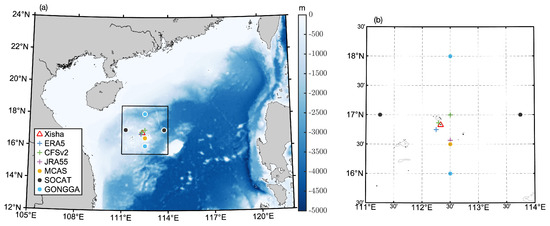
Figure 1. (a) Location of Xisha Research Station (red triangle), along with the matched grid points (colored crosses and dots) from the six data products under evaluation. The bathymetry of the northern South China Sea (SCS) is filled in on the map, and the bathymetry data is sourced from ETOPO2. (b) Enlarged panel of the black box in (a).

The dataset mainly includes air–sea flux components based on the eddy covariance method (ECM) such as latent heat flux, sensible heat flux, momentum flux, and carbon dioxide flux for 2016 at a 6 h resolution. It also provides corresponding meteorological variables such as wind speed, wind direction, air temperature, relative humidity, surface temperature, shortwave radiation, and longwave radiation covering the period from 2016 to 2020 at a 30 min resolution. All variables observed above were subjected to rigorous quality control and assurance procedures to ensure data integrity and reliability [10,30]. This dataset covers the period from 2016 to 2020 [29] and provides the community with a unique and informative data source for air–sea flux research near the northern SCS. In this study, we mainly used the observational outputs for 2016. The in situ observations used here have not yet been assimilated or included in any data products we selected for comparison.

2.2. Reanalysis Products

Three reanalysis datasets, simplified as ERA5, CFSv2 and JRA55, were chosen for evaluation. ERA5 is the fifth-generation global atmospheric reanalysis dataset developed by the European Centre for Medium-Range Weather Forecasts (ECMWF). It combines vast amounts of historical observations into global estimates using advanced modeling and data assimilation systems; it provides continuous atmospheric, land, and oceanic climate variables from 1940 to the present; and is now widely used in weather event analysis, model evaluation, renewable energy resource assessment, and numerous related climate studies [7,9]. We downloaded the datasets with a spatial resolution of 0.25° × 0.25° and a temporal resolution in hours.

CFSv2 (Climate Forecast System Version 2) was developed by the National Centers for Environmental Prediction (NCEP). It is a fully coupled ocean–atmosphere system built on the MOM4 ocean model, and it plays an important role in predicting short-term weather and investigating long-term climate change or extreme weather events. Data can be downloaded according to specific study demands [31]. Most of its variables use a spatial resolution of 0.205° × 0.204°, except for relative humidity, which has a resolution of 0.5° × 0.5°, and an hourly temporal resolution.

JRA55 (Japanese 55-year Reanalysis) is a set of global atmospheric reanalysis data products developed by the Japan Meteorological Agency, with a spatial resolution of 0.563° × 0.562° and temporal resolution of 3 or 6 h [32]. JRA55 is also widely used to verify numerical models and reconstruct atmospheric circulation.

In order to carry out comparisons with observations from Xisha Research Station, the corresponding variables for 2016 were acquired, including wind speed, wind direction, surface temperature, sea surface temperature (SST), air temperature, relative humidity, longwave/shortwave/net radiation, latent/sensible heat flux, and momentum flux. Since only ERA5 provides surface temperatures, the bulk SST from CFSv2 and JRA55 were corrected for surface temperature through the COARE 3.6 algorithm.

2.3. Carbon Flux Products

Three global carbon flux products, namely the Multi-observation Carbon Assimilation System (MCAS), Surface Ocean CO₂ Atlas (SOCAT), and Global ObservatioN-based system for monitoring Greenhouse GAses (GONGGA) inversion carbon flux dataset, were selected for comparisons with the air–sea surface CO₂ flux observed at Xisha Research Station and to assess their performance for the northern SCS. All of these products have undergone quality control and assimilation processing, providing important data support for the study of global carbon cycling and climate change, as well as supporting carbon-related flux assessment and environmental policy formulation [1,16,21].

MCAS is a global carbon flux assimilation product jointly developed by Tsinghua University and Peking University. It is based on the assimilation of the GEOS-Chem model and multisource observation data, comprising ground station observations and Orbiting Carbon Observatory-2 (OCO-2) satellite CO₂ data, and it integrates observed and remote sensing data. The carbon fluxes estimated with the MCAS have demonstrated significant advantages over control experiments that assimilate only in situ or satellite observations and other similar products [16]. In this study, daily CO₂ fluxes with a 1° × 1° resolution assimilating both in situ and satellite observations made during 2016 were used in comparisons with observations from Xisha Research Station.

SOCAT contains quality-controlled in situ ocean surface CO₂ measurements from ships, moorings, sailing yachts, and autonomous and drifting surface platforms for the global oceans and coastal seas from 1957 [20,33]. This dataset has a spatial resolution of 2° latitude × 2.5° longitude and a temporal resolution of 1 day. This dataset is continuously updated and enables detailed quantification of ocean carbon sinks, ocean acidification, and the evaluation of ocean biogeochemical models [1,34].

GONGGA is a set of observation-constrained global terrestrial ecosystem and ocean carbon flux products for 2015–2022, released by the Qinghai–Tibet Plateau Research Institute of the Chinese Academy of Sciences [21,35]. The dataset is based on the independently developed global atmospheric CO₂ inversion system “Gongga”, which assimilates the latest OCO-2 satellite CO₂ column concentration data. These data can effectively characterize the spatiotemporal patterns of carbon fluxes on global and regional scales. The time coverage is from 2015 to 2022, with a spatial resolution of 2° latitude × 2.5° longitude and a temporal resolution of 3 h. The “Gongga” system was continuously used in the Global Carbon Project in 2022 and 2023, excelling in the inversion of key assessment indicators and providing crucial support for the atmospheric inversion results of the Global Carbon Project.

2.4. Data Processing and Evaluation Metrics

Gridded hourly/daily variables from three reanalysis and carbon flux products need to be paired with the in situ observations. Two approaches are generally used to build the time series of certain variables in a fixed position from grid products. One selects the nearest grid point to the station as a proxy which was used in previous studies [18,28,30]. The other method involves calculating the spatial average of four or a few nearest points within the grid cell containing the target observation station. Empirical analysis shows that both methods produce consistent results in flux estimation [28,36]. This study employed a multipoint interpolation scheme for CO₂ flux, specifically in SOCAT and GOGGA. For other variables, we adopted the values of the closest grid or the mean values of the two closest grids from the selected datasets as proxies to compare against the observations, as shown in Figure 1 with plus signs and colored dots.

At the same time, an average of high-frequency observations at Xisha Research Station over time is still needed. Time averaging helps filter out high-frequency fluctuations that are not resolved in the reanalysis products. The observed meteorological variables are resampled every six hours, the momentum and heat flux data are compared at a temporal resolution of an hour, and the air–sea CO₂ fluxes are compared every day.

Specifically, we selected data within the time range from January 2016 to December 2016 (to match the observed carbon flux data at Xisha Research Station) and calculated the differences between the selected reanalysis products and observations. Commonly used error metrics were applied for evaluation, including the mean bias (Bias), root mean square error (RMSE), Pearson’s correlation coefficient (R), standard deviation (STD), and centered root mean square deviation (RMSD). Note that the last three were used in a Taylor diagram. The corresponding mathematical formulas are as follows:

$$Bias={\displaystyle \frac{1}{N}}\sum _{i=1}^N\left(E_i-O_i\right),$$

(1)

$$RMSE=\sqrt{{\displaystyle \frac{1}{N}}\sum _{i=1}^N{(E_i-O_i)}^2},$$

(2)

$$R={\displaystyle \frac{{\sum }_{i=1}^N(E_i-\overline{E})(O_i-\overline{O})}{\sqrt{{\sum }_{i=1}^N{(E_i-\overline{E})}^2}\sqrt{{\sum }_{i=1}^N{(O_i-\overline{O})}^2}}},$$

(3)

$$STD=\sqrt{{\displaystyle \frac{1}{N}}\sum _{i=1}^N{\left(E_i-\overline{E}\right)}^2},$$

(4)

$$RMSD=\sqrt{{\displaystyle \frac{1}{N}}\sum _{i=1}^N{[(E_i-\overline{E})-(O_i-\overline{O})]}^2},$$

(5)

where E represents the values of the aforementioned datasets under evaluation, O represents the observation values from Xisha Research Station, N is the total effective matching number, and the bar over the parameters stands for the mean value.

Kernel density estimation is also used here, as an application of kernel smoothing for probability density estimation, which can be expressed as

$$\hat{f}(z_x,z_y)={\displaystyle \frac{1}{N,h_x{h}_y}}\sum _{i=1}^{N}K\left({\displaystyle \frac{z_x-E_i}{h_x}}\right)K\left({\displaystyle \frac{z_y-O_i}{h_y}}\right),$$

(6)

where $z_x$ and $z_y$ represent the coordinates in the magnitude of E and O, respectively, and a continuous density distribution $\hat{f}$ is generated via grid-based computation. $h_x$ and $h_y$ are the bandwidth parameters for E and O, controlling the smoothing scale in each dimension. K(·) is the kernel function that assigns weights based on the distance between the data points and the target point, expressed as $K\left(u\right)={\displaystyle \frac{1}{\sqrt{2\pi }}}exp\left(-{\displaystyle \frac{1}{2}}{u}^2\right)$ for the Gaussian kernel.

3. Results

3.1. Comparison of Meteorological Variables

Comparisons of related meteorological variables can validate the quality of the air–sea fluxes. Figure 2 illustrates the daily time series of (a) wind speed (WS), (b) wind direction (WD), (c) surface temperature (T_s), (d) air temperature (T_a), and (e) relative humidity (RH) observed at Xisha Research Station during 2016, highlighted in red. The daily time series of these variables from ERA5 (blue), CFSv2 (green), and JRA55 (purple) are plotted for comparison.

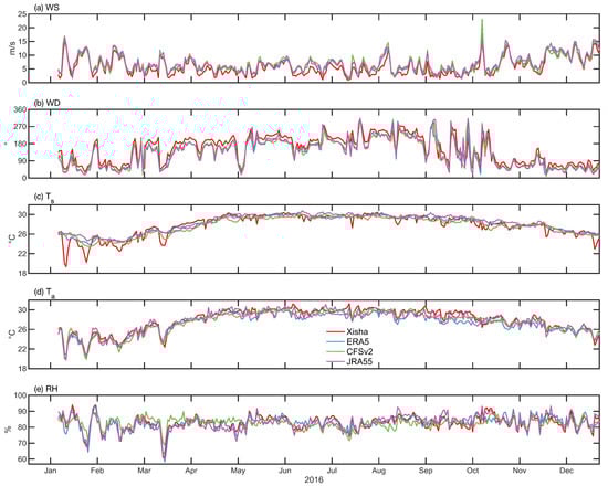
Figure 2. Daily time series of (a) wind speed (WS, m/s), (b) wind direction (WD, °), (c) surface temperature (${\mathrm{T}}_{\mathrm{s}}$, °C), (d) air temperature (${\mathrm{T}}_{\mathrm{a}}$, °C), and (e) relative humidity (RH, %) from Xisha Research Station (red) and reanalysis datasets (blue for ERA5, green for CFSv2, and purple for JRA55). Note that there are no effective observed values in early January.

As shown in Figure 2a,b, the wind is stronger and prevailing from the north in winter, but weaker and prevailing from the south in summer. Three reanalysis datasets highly correlated with the observed wind speed and wind direction, except in mid-October, during the period of Typhoon Sarika (2016), which passed through the south of Yongxing Island. This resulted in the largest wind speed bias in CFSv2, which is much larger than the observed values. The observed ${\mathrm{T}}_{\mathrm{s}}$ and ${\mathrm{T}}_{\mathrm{a}}$ show consistent variation, especially in winter. However, reanalyses ${\mathrm{T}}_{\mathrm{s}}$ and ${\mathrm{T}}_{\mathrm{a}}$ show a different pattern in January and February, with general overestimation. A relatively larger deviation in ${\mathrm{T}}_{\mathrm{s}}$ is illustrated between the observed and reanalysis patterns (Figure 2c). Also, a previous study by Zhou et al. (2018) [10] pointed out the larger bias of ${\mathrm{T}}_{\mathrm{s}}$; the observed ${\mathrm{T}}_{\mathrm{s}}$ were obviously not captured with OAFlux. The OAFlux-estimated ${\mathrm{T}}_{\mathrm{s}}$ was retrieved using an advanced very-high-resolution radiometer (AVHRR) and is easily affected by the presence of clouds; thus, it only captures seasonal trends. Estimates from reanalysis always exclude some special synoptic signals, such as abrupt drops during cold air temperatures and typhoons or gradual temperature increases induced by the passage of a warm eddy. RH, which is similar to ${\mathrm{T}}_{\mathrm{a}}$, exhibits a larger fluctuation in winter and early spring.

The observed daily time series of (a) downward shortwave radiation (DSR), (b) upward shortwave radiation (USR), (c) downward longwave radiation (DLR), (d) upward longwave radiation (ULR), and (e) net radiation (Rn) obtained at Xisha Research Station are illustrated in Figure 3 with solid red lines. The corresponding daily time series from ERA5 (blue), CFSv2 (green), and JRA55 (purple) are shown for comparison.

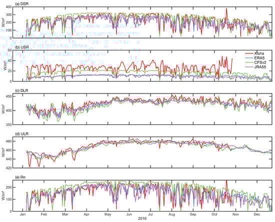
Figure 3. Same as Figure 2, but for (a) downward shortwave radiation (DSR, ${\mathrm{W}/\mathrm{m}}^2$), (b) upward shortwave radiation (USR, ${\mathrm{W}/\mathrm{m}}^2$), (c) downward longwave radiation (DLR, ${\mathrm{W}/\mathrm{m}}^2$), (d) upward longwave radiation (ULR, ${\mathrm{W}/\mathrm{m}}^2$), and (e) net radiation (Rn, ${\mathrm{W}/\mathrm{m}}^2$).

The observed longwave radiation demonstrates evident seasonal variation (Figure 3c,d), both upward and downward. Although shortwave radiation has a lower magnitude than longwave radiation, it displays greater variability (Figure 3a,b). Longwave radiation, on the contrary, presents a relatively larger variability during cold seasons and remains relatively stable in warmer seasons.

The three reanalysis products reproduce the variation in DSR and DLR well, but with larger deviation for ULR and especially USR. CFSv2 significantly overestimates DSR, while ERA5 and JRA55 slightly underestimate it. All three reanalysis products underestimate USR and its intramonth variability, with minimal bias from CFSv2 and large bias from ERA5 and JRA55. For ULR, the observations show significant fluctuations from January to March, which are not reflected in the three products.

To systemically evaluate the performance of the reanalysis products, a very useful evaluation tool called the Taylor diagram was applied to quantify the deviation between the observations and the three reanalysis datasets. The Taylor diagram simultaneously provides key statistics, including R, STD, and RMSD, as shown in Figure 4. The angle of radial lines in the Taylor diagram corresponds to the correlation coefficient, while the length between any point and the origin indicates the amplitude of fluctuation, which is represented by one STD of the data. The results show that ERA5 performs best for multiple variables: The wind speed (R = 0.95, RMSD = 0.98 m/s) and wind direction (R = 0.95, RMSD = 22.01°) are the most accurate. ${\mathrm{T}}_{\mathrm{s}}$ (R = 0.93, RMSD = 0.88° C) and radiation variables (DSR: R = 0.82, RMSD = 42.42 ${\mathrm{W}/\mathrm{m}}^2$; DLR: R = 0.93, RMSD = 5.94 ${\mathrm{W}/\mathrm{m}}^2$; ULR: R = 0.93, RMSD = 5.43 ${\mathrm{W}/\mathrm{m}}^2$) are also similar to the observation, but with a relatively low correlation with USR (R = 0.58 RMSD = 6.44 ${\mathrm{W}/\mathrm{m}}^2$), finally resulting a middle-level correlation in net radiation (R = 0.77, RMSD = 36.49 ${\mathrm{W}/\mathrm{m}}^2$). However, CFSv2 does not perform well in shortwave radiation, both upward and downward, with the lowest correlation and highest standard deviation. JRA55 has an advantage in RH (R = 0.86, RMSD = 2.33%), but also does not perform well in USR. Overall, the three reanalysis products show similar performances in WS, WD, ${\mathrm{T}}_{\mathrm{s}}$, ${\mathrm{T}}_{\mathrm{a}}$, and ULR, with three error indicators always clustered together in the Taylor diagram. For the other variables, ERA5 and JRA55 behaved more consistently with the observed values, while CFSv2 presents a relatively larger inconsistency.

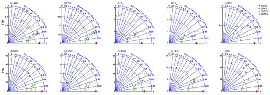
Figure 4. Taylor diagram of (a) wind speed (WS, m/s), (b) wind direction (WD, °), (c) surface temperature (${\mathrm{T}}_{\mathrm{s}}$, °C), (d) air temperature (${\mathrm{T}}_{\mathrm{a}}$, °C), (e) relative humidity (RH, %), (f) downward shortwave radiation (DSR, ${\mathrm{W}/\mathrm{m}}^2$), (g) upward shortwave radiation (USR, ${\mathrm{W}/\mathrm{m}}^2$), (h) downward longwave radiation (DLR, ${\mathrm{W}/\mathrm{m}}^2$), (i) upward longwave radiation (ULR, ${\mathrm{W}/\mathrm{m}}^2$), and (j) net radiation (Rn, ${\mathrm{W}/\mathrm{m}}^2$) observed at Xisha Research Station compared with ERA5, CFSv2, and JRA55. As above, red indicates observation results; blue, ERA5; green, CFSv2; and purple, JRA55.

To minimize the potential influences associated with temporal scale effects, the monthly statistical metrics of the above ten state variables between the observations and three reanalysis datasets were quantified. As indicated in Table 1, all correlation coefficients (R) are statistically significant. Here, a common significance level ($\alpha$ = 0.05) was used, and all p-values were less than $\alpha$. All reanalysis datasets maintained a high correlation coefficient (R) with the observations, larger than 0.9 across most meteorological variables, except in RH and USR. The performance at the monthly time scale is generally consistent with the daily one but with a slight difference in values. It is noted that CFSv2 estimations present better performance in ${\mathrm{T}}_{\mathrm{s}}$ and USR, with the lowest Bias and RMSE, largely due to its fully coupled ocean–atmosphere dynamics. Wind speed (WS) and air temperature (${\mathrm{T}}_{\mathrm{a}}$) are generally overestimated in the reanalysis datasets, while the remaining variables tend to be underestimated. Wind speed (WS) and air temperature (${\mathrm{T}}_{\mathrm{a}}$) are generally overestimated in reanalysis datasets, while other variables tend to be underestimated.

Table 1. Monthly mean evaluation metrics between observed and reanalysis patterns.

Metrics	Products	WS	WD	${\mathrm{T}}_{\mathrm{s}}$	${\mathrm{T}}_{\mathrm{a}}$	RH	DSR	USR	DLR	ULR	Rn
	ERA5	1.07	−18.49	0.32	−0.65	−0.02	−8.86	−15.15	−6.44	−0.48	−1.29
Bias	CFSv2	1.12	−18.27	0.05	−0.34	−0.24	26.11	−8.92	−8.64	−0.62	29.53
	JRA55	1.19	−17.79	0.50	−0.21	−0.05	−22.89	−16.20	−6.10	2.48	−16.10
	ERA5	1.10	19.34	0.61	0.73	0.94	13.51	15.28	6.94	3.04	8.12
RMSE	CFSv2	1.21	19.84	0.67	0.41	1.71	33.12	9.28	9.65	4.15	34.21
	JRA55	1.22	19.67	0.81	0.32	1.24	27.77	16.34	6.51	4.37	22.09
	ERA5	0.994	0.995	0.987	0.994	0.879	0.973	0.698	0.983	0.993	0.982
R	CFSv2	0.976	0.991	0.960	0.995	0.421	0.965	0.629	0.958	0.965	0.946
	JRA55	0.990	0.989	0.963	0.994	0.881	0.937	0.618	0.986	0.977	0.913

3.2. Comparison of Heat and Momentum Fluxes

As displayed in Figure 5, time series of air–sea (a) sensible heat flux (SHF), (b) latent heat flux (LHF), and (c) momentum flux (TAU) from the observations at Xisha Research Station and their paired fluxes from ERA5, CFSv2, and JRA55 are positively correlated in general. Like above, the red dots in Figure 5 represent the observations, and the corresponding hourly series of ERA5, CFSv2, and JRA55 are marked with blue, green, and purple dots, respectively. From this, we can see that the LHF, SHF, and TAU range from −50 to 800 ${\mathrm{W}/\mathrm{m}}^2$, from −50 to 250 ${\mathrm{W}/\mathrm{m}}^2$, and from 0 to 0.8 N/m², respectively, throughout 2016. The gray dotted and dashed line in Figure 5 indicates the period of missing values, from 1 April to 21 June. Note that positive values for LHF or SHF represent the heat released by the ocean into the atmosphere, and TAU is always positive, meaning that the atmosphere transfers kinetic energy to the ocean.

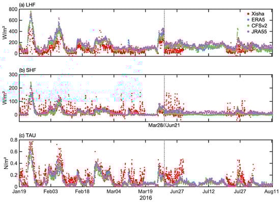
Figure 5. Time series of hourly (a) latent heat flux (LHF, ${\mathrm{W}/\mathrm{m}}^2$), (b) sensible heat flux (SHF, ${\mathrm{W}/\mathrm{m}}^2$), and (c) momentum flux (TAU, ${\mathrm{N}/\mathrm{m}}^2$) from Xisha Research Station and reanalysis datasets (ERA5, CFSv2, and JRA55). The gray dotted and dashed line stands for the period of missing values, from 1 April to 21 June.

As shown in Figure 5, the three reanalysis datasets generally agree well with the observations, but systematically overestimate the LHF while underestimating the SHF and TAU, while the largest deviation occurs in the SHF. The annual evolution of air–sea heat and momentum fluxes at Xisha Research Station, regardless of whether obtained from the observed or reanalysis datasets, exhibits obvious seasonal variation, with maximum values primarily observed in January, which is largely attributed to a higher sea–air thermal contrast and enhanced winds associated with cold air outbreaks in winter.

ERA5, CFSv2, and JRA55 exhibit a relatively high consistency in capturing the seasonal variability in LHF, SHF, and TAU. However, the observed values of SHF exhibit greater variability than the three reanalysis datasets, which is potentially due to the high sample frequency of the observed measurements.

For the spikes in SHF shown in Figure 5b, the higher temporal variability and more pronounced diurnal cycle in observations reflect inherent turbulent processes that are inherently difficult to capture in reanalysis datasets, which is possibly a consequence of the turbulent exchange coefficient being influenced by water depth, which is currently not reflected in the parameterization. These spikes appear in both winter and summer. This discrepancy is also related to the bias in ${\mathrm{T}}_{\mathrm{s}}$.

Scatterplots of the heat and momentum flux between the observations and the three reanalysis datasets are presented in Figure 6, and the quantitative errors between them are indicated in each panel. There are clear positive relationships between the three reanalysis datasets and observed fluxes. For LHF, all three reanalysis datasets exhibit systematic positive biases relative to observations. Among them, CFSv2 holds the minimum RMSE as 90.50 ${\mathrm{W}/\mathrm{m}}^2$ but the lowest correlation coefficient as 0.714. For SHF, a lower correlation coefficient between the observation and three reanalysis, in which ERA5 holds the minimum RMSE at 33.35 ${\mathrm{W}/\mathrm{m}}^2$ with R=0.418. For TAU, a general underestimate also appears in the scatterplots, in which JRA55 has a minimum RMSE at 0.110 ${\mathrm{N}/\mathrm{m}}^2$ with the highest correlation (R = 0.760). Meanwhile, the specific numerical values of error metrics across the three reanalysis datasets, particularly the SHF and TAU indicators, exhibit a high degree of consistency. Filled colors stand for the kernel density calculated by Formula (6), which not only illustrates the agreement between the observation and the three reanalysis datasets but also reveals the differences in the performance of ERA5, CFSv2, and JRA55.

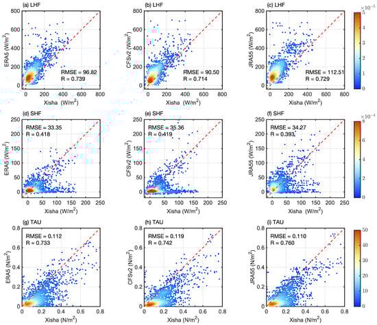
Figure 6. Scatter density and error statistics for (a–c) LHF (${\mathrm{W}/\mathrm{m}}^2$), (d–f) SHF (${\mathrm{W}/\mathrm{m}}^2$), and (g–i) TAU (${\mathrm{N}/\mathrm{m}}^2$) between the observations and the three reanalysis datasets. The filled colors represent kernel density estimates of the scatter point distributions, indicating the relative concentration of data in two-dimensional space. RMSE and R are indicated in the corner of each panel. All p-values of R are less than 0.05.

Note that similar bulk algorithms were adopted by all three reanalysis datasets. However, for the observed air–sea heat/momentum fluxes, the eddy covariance method was used, the difference in methods potentially led to the systematic negative/positive biases between the observations and reanalysis datasets. Zhou et al. (2018) [10] discussed possible effects of bulk variables on the biases in the SHF and LHF. They concluded that bias in the air-specific humidity near the sea surface is the most dominant factor for determining the biases in LHF during the spring and winter. Both biases in air-specific humidity and wind are responsible for controlling the biases in LHF during the summer–autumn period. Biases in ${\mathrm{T}}_{\mathrm{s}}$ are responsible for controlling those in SHF, and the effects of biases in ${\mathrm{T}}_{\mathrm{s}}$ on those in SHF during the spring and winter are much greater than those in the summer–autumn period. Differences in the air relative humidity and wind speed contribute to latent heat flux discrepancies, while differences in sensible heat flux are likely due to contrasts in air temperature and sea surface temperature. Specific quantitative statistics must be investigated further to clarify their impacts.

Table 2 presents a quantitative analysis of the hourly deviation between the observed ECM fluxes and the bulk fluxes from three reanalysis, by subtracting ECM fluxes from bulk fluxes. For LHF, the mean values of hourly deviation range from 53.61 ${\mathrm{W}/\mathrm{m}}^2$ for CFSv2 to 82.50 ${\mathrm{W}/\mathrm{m}}^2$ for JRA55, with the STD of hourly deviation ranging from 71.81 ${\mathrm{W}/\mathrm{m}}^2$ for ERA5 to 76.52 ${\mathrm{W}/\mathrm{m}}^2$ for JRA55. The CFSv2 error metric falls within the middle range. For SHF, the mean values of hourly deviation range from −13.78 ${\mathrm{W}/\mathrm{m}}^2$ for CFSv2 to −1.99 ${\mathrm{W}/\mathrm{m}}^2$ for JRA55; the STDs of hourly deviation range from 31.35 ${\mathrm{W}/\mathrm{m}}^2$ for ERA5 to 34.23 ${\mathrm{W}/\mathrm{m}}^2$ for JRA55, with CFSv2 exhibiting the lowest error metrics. For TAU, the mean values of hourly deviation range from −0.080 ${\mathrm{N}/\mathrm{m}}^2$ for CFSv2 to −0.066 ${\mathrm{N}/\mathrm{m}}^2$ for ERA5; the STDs of hourly deviation range from 0.086 ${\mathrm{N}/\mathrm{m}}^2$ for JRA55 to 0.090 ${\mathrm{N}/\mathrm{m}}^2$ for ERA5. In general, considerable uncertainties exist between the eddy covariance method and bulk flux algorithms. Therefore, research investigating these biases [8,9,18] is on the rise.

Table 2. Statistical metrics of the hourly deviation between the observed ECM fluxes and bulk fluxes from reanalysis.

Metrics	Products	LHF	SHF	TAU
	ERA5	65.96	−11.41	−0.066
Bias	CFSv2	53.61	−13.78	−0.080
	JRA55	82.50	−1.99	−0.069
	ERA5	71.81	31.35	0.090
STD	CFSv2	72.93	32.58	0.088
	JRA55	76.52	34.23	0.086

Further quantitative analysis of the discrepancy between the observed eddy covariance fluxes and the bulk fluxes from reanalysis remains limited, to elucidate the underlying physical mechanisms, incorporating additional variables is necessary.

3.3. Comparison of CO₂ Fluxes

The air–sea CO₂ fluxes from the selected products were all converted to the same unit, $\mathsf{\mu }{\mathrm{mol}/\mathrm{m}}^2/\mathrm{s}$, for comparison with the observations. Figure 7 illustrates the observed daily mean air–sea CO₂ flux at Xisha Research Station, from January to September 2016, along with the time series of CO₂ flux from MCAS (orange), SOCAT (black), and GONGGA (cyan) for comparison. Note that GONGGA is displayed in three-hour intervals, while MCAS and SOCAT are displayed in one-day intervals; these resolutions correspond to their original temporal resolutions, respectively.

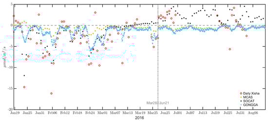
Figure 7. Daily means of the air–sea CO₂ flux observed at Xisha Research Station (red circles), along with corresponding time series from MCAS (orange dots), SOCAT (black dots), and GONGGA (cyan dots).

As shown in Figure 7, large spikes of CO₂ flux discrepancies generally occurred. The time values from MCAS and GONGAA are very small, whereas the observed CO₂ fluxes are relatively larger. The discrepancies tend to be larger when the observed fluxes are large but positive (June to August) than when large and negative (January to March). The observed air–sea CO₂ flux at Xisha Research Station exhibits a clear seasonal variation, with a daily mean value of 0.88 $\mathsf{\mu }{\mathrm{mol}/\mathrm{m}}^2/\mathrm{s}$ in summer (June–August) and −3.01 $\mu {\mathrm{mol}/\mathrm{m}}^2/\mathrm{s}$ in winter and spring (January–April), indicating that this region of the SCS mainly acts as a carbon source in warm seasons and a carbon sink in cold seasons. Compared with the gridded products from MCAS, SOCAT, and GONGGA, a large discrepancy can be found on the daily time scale.

The statistical parameters, Bias, RMSE, and R, are listed in Table 3. Referring to Figure 7 and Table 3, it can be easily observed that SOCAT performed best with a correlation coefficient of 0.75 (Bias = 1.36 $\mu {\mathrm{mol}/\mathrm{m}}^2/\mathrm{s}$, RMSE = 3.02 $\mu {\mathrm{mol}/\mathrm{m}}^2/\mathrm{s}$), and GONGGA shows a correlation of 0.64 (Bias = 0.57 $\mu {\mathrm{mol}/\mathrm{m}}^2/\mathrm{s}$, RMSE = 3.28 $\mu {\mathrm{mol}/\mathrm{m}}^2/\mathrm{s}$), while MCAS had the lowest correlation coefficient of only 0.36 (Bias = 0.87$\mu {\mathrm{mol}/\mathrm{m}}^2/\mathrm{s}$, RMSE = 3.7 $\mu {\mathrm{mol}/\mathrm{m}}^2/\mathrm{s}$). The daily CO₂ fluxes from MCAS and GONGGA are always in the opposite phase to the observations and SOCAT after June.

Table 3. Statistical metrics for CO₂ flux evaluation.

Metrics	MCAS	SOCAT	GONGGA
Bias	0.87	1.36	0.57
RMSE	3.70	3.02	3.28
R	0.36	0.75	0.64

Direct measurements of turbulent fluxes are very challenging and precious. Continuous in situ observations usually capture small-scale processes near the sea surface, through are very limited in spatial coverage. The variation in CO₂ flux in marginal seas is significantly related to the progress of the coastal dynamics from small to large time and space scales. The ocean is always treated as a strong source in summer, with a gradual decrease in strength over fall and into winter [3]. The three carbon flux datasets can be compared to assess the seasonal mean state of the reconstructed air–sea CO₂ flux in spatial distribution patterns. The monthly (February and August) and annual mean distributions of air–sea CO₂ flux during 2016 from the three carbon flux datasets are illustrated in Figure 8.

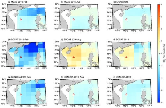
Figure 8. Monthly and annual mean states of air–sea CO₂ flux from MCAS, SOCAT, and GONGGA in the northern SCS. Like in Figure 1, the red triangle represents Xisha Research Station.

Assimilation with OCO-2, MCAS and GONGGA yields similar spatiotemporal patterns in both February and August, even in the annual mean state.However, when also assimilating in situ surface ocean CO₂ measurements, the distribution of CO₂ flux in SOCAT is significantly different from those of MCAS and GONGGA (Figure 8d–f). This partly explains the better performance of SOCAT in Figure 7. The deviations in spatial distribution between the three carbon products also indicate potential large differences between in situ and remote sensing measurements and other techniques for surface ocean CO₂ flux estimation.

In general, SOCAT is broadly consistent with the in situ observations from Xisha Research Station. However, MCAS and GONGGA still suffer large biases, especially in the seasonal transition. The above analyses indicate that the mean state of air–sea CO₂ flux in the newly established dataset shows an obvious difference in monthly spatial distributions.

4. Discussion

Bulk flux algorithms are theoretically founded in Monin–Obukhov similarity theory. Various bulk algorithms have been developed and used in models and reanalysis datasets. However, many aspects of the algorithms are empirical. The algorithm used in ERA5 is the ECMWF scheme (Beljaars, 1995) [37], in CFSv2 it is the UA (The University of Arizona algorithm; Brunke et al., 2002; Zeng et al., 1998) [38,39], in JRA55 it is a similar algorithm known as Beljaars, 1995 [37], with modifications (Smith et al., 2011) [40].

The eddy covariance method is the most accurate method for measuring air–sea fluxes, but it is also the most expensive and complex. It relies on measurements of wind velocity, temperature, and scalar quantities like humidity or CO₂ concentration at scales much faster than the evolution of eddies, typically at 10 or 20 Hz. Its implementation requires very precise, fast-response instruments to capture high-frequency turbulent fluctuations [41].

Installed the eddy covariance instruments in a fixed station can effectively minimize the errors caused by flow distortion and motion correction. All of the sensors at Xisha Research Station have been checked via pre- and post-installment calibrations by the National Center of Ocean Standards and Metrology [10].

Previous studies have provided insightful scientific guidance for selecting flux products for different applications and characterized advances in the global datasets of air–sea turbulent heat flux. Cronin et al. (2019) [8] reviewed the capabilities of the measurements and their accuracy of heat and momentum flux, which pointed out that cross-platform and cross-product intercomparisons must be conducted, and differences must be reconciled. Yu and Weller (2007) [42] also noted that direct flux measurements are available only at limited locations. Air–sea fluxes are commonly estimated from bulk flux parameterization using flux-related near-surface meteorological variables (winds, sea and air temperatures, and humidity) that are available from buoys, ships, satellite remote sensing, numerical weather prediction models, and/or a combination of any of these sources. Tang et al. (2024) [9] comprehensively reviewed the accuracy and spatiotemporal patterns of 15 global products of air–sea turbulent heat flux from 1988 to 2020. All of these studies concluded that most products show consistent annual to seasonal trends of heat and momentum fluxes, with larger discrepancies at lower latitudes for heat fluxes and larger discrepancies at high latitudes for momentum fluxes. The interseasonal variations in LHF and SHF are more pronounced in the Northern Hemisphere than in the Southern Hemisphere. Uncertainties in parameterization-based flux estimates are large, and when they are integrated over the ocean basins, they cause a large imbalance in the global ocean budgets.

The following three tables summarize the basic statistics of all the variables we used, including observations (simplified as Xisha) and six selected data products. Their mean values, STDs, and 95% confidence intervals are listed in Table 4, Table 5 and Table 6, where the differences between the observations and data products are quantified. Here, we used $\pm 1.96\delta$ as the range limit of the 95% confidence interval, where $\delta$ equals the STD. These statistics corroborate our earlier research findings and indirectly attest the high quality of the observational data.

Table 4. Statistical metrics of meteorological variables from observation and reanalysis.

Metrics	Products	WS	WD	${\mathrm{T}}_{\mathrm{s}}$	${\mathrm{T}}_{\mathrm{a}}$	RH	DSR	USR	DLR	ULR	Rn
Mean	Xisha	5.74	150.16	27.80	27.88	82.75	220.16	25.84	426.62	468.70	164.90
	ERA5	6.80	132.06	28.05	27.21	82.83	211.80	10.22	419.90	466.34	155.14
	CFSv2	6.84	132.33	27.75	27.51	82.59	247.44	16.05	417.77	465.96	183.21
	JRA55	6.92	133.00	28.22	27.68	82.67	196.79	9.07	420.33	468.99	139.07
STD	Xisha	3.09	70.44	2.20	2.28	4.43	74.31	7.50	16.06	14.16	56.60
	ERA5	2.99	70.33	1.74	2.03	4.31	58.28	2.34	16.17	10.72	52.24
	CFSv2	3.11	69.20	1.82	2.22	3.09	79.90	5.31	18.68	11.23	66.22
	JRA55	3.12	73.94	1.80	2.24	4.48	60.50	2.37	15.18	11.23	55.39

Table 5. Statistical metrics of heat and momentum fluxes from observation and reanalysis.

Metrics	Products	LHF	SHF	TAU
Mean	Xisha	83.10	27.97	0.17
	ERA5	139.24	13.30	0.10
	CFSv2	128.97	10.87	0.08
	JRA55	161.55	23.05	0.09
STD	Xisha	82.38	33.56	0.13
	ERA5	100.56	21.67	0.10
	CFSv2	100.41	26.51	0.10
	JRA55	104.17	27.94	0.10
Confidence Interval (95%)	Xisha	[−78.37, 244.57]	[−37.82, 93.75]	[−0.09, 0.43]
	ERA5	[−57.86, 336.33]	[−29.17, 55.77]	[−0.10, 0.29]
	CFSv2	[−67.84, 325.78]	[−41.09, 62.83]	[−0.11, 0.27]
	JRA55	[−42.63, 365.74]	[−31.72, 77.82]	[−0.11, 0.29]

Table 6. Statistical metrics of CO₂ flux from observation and reanalysis.

Metrics	Products	CO2 Flux
Mean	Xisha	−2.02
	MCAS	−1.21
	GONGGA	−1.43
	SOCAT	0.07
STD	Xisha	5.09
	MCAS	1.16
	GONGGA	1.14
	SOCAT	3.08
Confidence Interval (95%)	Xisha	[−11.99, 7.96]
	MCAS	[−3.49, 1.07]
	GONGGA	[−3.67, 0.81]
	SOCAT	[−5.97, 6.10]

The strong cooling of wintertime surface temperature observed at the Yongxing Island site arises from localized processes that are not fully resolved in coarse resolution reanalysis products. The monitoring tower, situated on a shallow southwestern reef flat (∼5–10 m), is always affected by stronger coast parallel northeasterly winds in wintertime, which possibly promote full-depth turbulent mixing and potentially trigger coastal upwelling. If these mechanisms substantially amplify surface cooling, the surface temperature is likely to gradually approach the air temperature. However, further evidence from coastal currents and hydrological states are needed to validate above assumption. Furthermore, open ocean conditions may well be represented by reanalysis datasets, but for complex coastal progresses, such as upwelling, are always poorly captured due to relative coarse spatial resolution. This also reasonably explains the occasional significant discrepancy between reanalysis data and in situ point observations in shallow coastal environments.

Systematic overestimation or underestimation of heat and momentum flux persists in the widely used ERA5, CFSv2, and JRA55 products, though there is relatively high agreement in the flux-related variables compared to in situ observations. Numerical weather prediction models have known biases in the ocean surface fluxes, which can be attributed to the biases in the SSTs used to force the models, biases in the atmospheric model physics, and biases in the ocean model physics [8,14,43]. This has placed great importance on the observation in situ air–sea fluxes.

The potential influences of island on turbulent fluxes were validated by Zhou et al. (2017) [30] and Zhang et al. (2021) [11]. The eddy covariance method employed through enhanced data processing is well suited to the fixed stations located near similar islands and reefs. Comparing in situ observations with grid products at a 1/4 to 1/2 km resolution remains an issue, and although the differences can be minimized, they cannot be avoided.

Due to the limitation of observation stations, only one site location in the northeastern South China Sea was compared in this study, restricted the applicability of our results. More observation stations near coastal seas are essential, in order to better monitoring and understanding the exchange of air–sea fluxes near shores, and improving the accuracy and reliability of data products. With the advancement of artificial intelligence and deep learning technologies, high-spatiotemporal-resolution ocean datasets have proliferated rapidly. The validation and evaluation of these datasets urgently require observational verification.

5. Conclusions

Using air–sea heat flux, momentum flux, CO₂ flux, and associated meteorological variables obtained from a fixed tower at Xisha Research Station in the northern SCS, three reanalysis products (ERA5, CFSv2, and JRA55) and three global carbon products (MCAS, SOCAT, and GONGGA) were evaluated. The main conclusions are as follows.

The comparison of the meteorological variables indicates that the three reanalysis data products generally agree well with the observations. On the daily scale, ERA5 performed better for the wind, surface temperature, and radiation variables. Meanwhile, CFSv2 performed particularly well for air temperature (R = 0.96), while JRA55 performed better for relative humidity (R = 0.86) (Figure 4). On the monthly scale, the biases further reduced, and seasonal variations were well captured, with the exception of relatively larger deviations occurring when strong cold air outbreaks (Table 1).

The evaluation of air–sea heat and momentum fluxes indicates that the three reanalysis data products exhibit similar systematic biases. In general, latent heat flux is more reliable than sensible heat flux; the former is generally overestimated with a high correlation coefficient above 0.71, while the latter is generally underestimated with a low correlation coefficient less than 0.42. For the momentum flux, overall underestimation with a high correlation coefficient larger than 0.73 were exhibit for the three reanalysis products. No clear superiority or inferiority was evident among the three reanalysis datasets. ERA5 displays the highest correlation for latent heat flux (R = 0.74) and the best performance for sensible heat flux (R = 0.42, RMSE = 33.35 ${\mathrm{W}/\mathrm{m}}^2$); JRA55 has a slight advantage for momentum flux (R = 0.76) and maintains the minimal mean bias for sensible heat flux at −1.99 ${\mathrm{W}/\mathrm{m}}^2$; while CFSv2 holds the minimal RMSE for sensible heat flux.

Regarding air–sea CO₂ flux, SOCAT aligns more closely with the observations and captures seasonal variations well, with a correlation coefficient of 0.75. GONGGA follows with 0.64, while MCAS had the lowest correlation coefficient of only 0.36. For the spatial pattern in the northern SCS, MCAS and GONGGA display a significant difference with SOCAT, particularly during the seasonal transition.

It is noteworthy that producing high-quality carbon flux products is challenging due to the complexity of the carbon cycle and the limitations of data sources. Through the assessment of global coastal ocean, air–sea CO₂ flux has advanced significantly over the past four decades, but critical knowledge gaps remain in understanding and quantifying coastal carbon fluxes and the underlying controls [3]. The increase in carbon absorbed by the ocean was linked with enhancement in carbon uptake capacity instead of the expansion of carbon sink areas [24]. Under realistic scenarios of increasing atmospheric CO₂ concentrations, both the magnitude and spatial patterns of air–sea CO₂ fluxes are likely to change [44]. Further extensive developments in ocean carbon observations are required, targeting global ocean CO₂ fluxes.

References

- Bunsen, F.; Nissen, C.; Hauck, J. The Impact of Recent Climate Change on the Global Ocean Carbon Sink. Geophys. Res. Lett. 2024, 51, e2023GL107030. [Google Scholar] [CrossRef]
- Yu, L. Global Air–Sea Fluxes of Heat, Fresh Water, and Momentum: Energy Budget Closure and Unanswered Questions. Annu. Rev. Mar. Sci. 2019, 11, 227–248. [Google Scholar] [CrossRef]
- Dai, M.; Su, J.; Zhao, Y.; Hofmann, E.E.; Cao, Z.; Cai, W.J.; Gan, J.; Lacroix, F.; Laruelle, G.G.; Meng, F.; et al. Carbon Fluxes in the Coastal Ocean: Synthesis, Boundary Processes, and Future Trends. Annu. Rev. Earth Planet. Sci. 2022, 50, 593–626. [Google Scholar] [CrossRef]
- Chen, Y.; Zhao, H.; Gao, H. Spatiotemporal Evolution of Air–Sea CO2 Flux in the South China Sea and Its Response to Environmental Factors. Remote Sens. 2024, 16, 4724. [Google Scholar] [CrossRef]
- Wang, X.; Zhang, R.; Huang, J.; Zeng, L.; Huang, F. Biases of five latent heat flux products and their impacts on mixed-layer temperature estimates in the South China Sea. J. Geophys. Res. Oceans 2017, 122, 5088–5104. [Google Scholar] [CrossRef]
- Luo, J.; Gao, Z.; Liu, K.; Song, X.; Wu, S.; Fang, Z. Evaluation of ERA-Interim and MERRA Sensible Heat Flux and Latent Heat Flux along Coast of China. Adv. MeT S&T 2018, 8, 6–14. (In Chinese) [Google Scholar] [CrossRef]
- Luo, S.; Liu, S.; Zhang, T.; Cai, D.; Zhao, T.; Han, J. Applicability Analysis of Three Reanalysis Data in Xisha Sea Area. Adv. Mar. Sci. 2022, 9, 96–107. (In Chinese) [Google Scholar] [CrossRef]
- Cronin, M.F.; Gentemann, C.L.; Edson, J.; Ueki, I.; Bourassa, M.; Brown, S.; Clayson, C.A.; Fairall, C.W.; Farrar, J.T.; Gille, S.T.; et al. Air-Sea Fluxes With a Focus on Heat and Momentum. Front. Mar. Sci. 2019, 6, 430. [Google Scholar] [CrossRef]
- Tang, R.; Wang, Y.; Jiang, Y.; Liu, M.; Peng, Z.; Hu, Y.; Huang, L.; Li, Z. A review of global products of air-sea turbulent heat flux: Accuracy, mean, variability, and trend. Earth-Sci. Rev. 2024, 249, 104662. [Google Scholar] [CrossRef]
- Zhou, F.; Zhang, R.; Shi, R.; Chen, J.; He, Y.; Wang, D.; Xie, Q. Evaluation of OAFlux datasets based on in situ air-sea flux tower observations over Yongxing Island in 2016. Atmos. Meas. Tech. 2018, 11, 6091–6106. [Google Scholar] [CrossRef]
- Zhang, R.; Zhou, F.; Wang, X.; Wang, D.; Gulev, S.K. Cool Skin Effect and its Impact on the Computation of the Latent Heat Flux in the South China Sea. J. Geophys. Res. Oceans 2021, 126, 2020JC016498. [Google Scholar] [CrossRef]
- Moura, R.; Casagrande, F.; de Souza, R.B. An Overview of Air-Sea Heat Flux Products and CMIP6 HighResMIP Models in the Southern Ocean. Atmosphere 2025, 16, 402. [Google Scholar] [CrossRef]
- Zhang, W.; Luo, G.; Hamdi, R.; Ma, X.; Termonia, P.; De Maeyer, P.; Chen, A. Bridging the Gap in Carbon Cycle Studies: Meteorological Station-Based Carbon Flux Dataset as a Complement to EC Towers. Agric. For. Meteorol. 2025, 362, 110397. [Google Scholar] [CrossRef]
- Small, R.J.; Bryan, F.O.; Bishop, S.P.; Tomas, R.A. Air–Sea Turbulent Heat Fluxes in Climate Models and Observational Analyses: What Drives Their Variability? J. Clim. 2019, 32, 2397–2421. [Google Scholar] [CrossRef]
- Anna, S. Turbulent fluxes of momentum and heat over land in the High-Arctic summer: The influence of observation techniques. Polar Res. 2014, 33, 21567. [Google Scholar] [CrossRef]
- Su, W.; Wang, B.; Chen, H.; Lin, Z.; Zheng, X.; Chen, S. A new global carbon flux estimation methodology by assimilation of both in situ and satellite CO2 observations. npj Clim. Atmos. Sci. 2024, 7, 1–10. [Google Scholar] [CrossRef]
- Yuan, Q.; Wang, X.; Che, T.; Li, J. Global carbon flux dataset generated by fusing remote sensing and multiple flux networks observation. Sci. Data 2025, 12, 1359. [Google Scholar] [CrossRef]
- Sivam, S.; Zhang, C.; Zhang, D.; Yu, L.; Dressel, I. Surface Latent and Sensible Heat Fluxes over the Pacific Sub-Arctic Ocean from Saildrone Observations and Three Global Reanalysis Products. Front. Mar. Sci. 2024, 11, 1431718. [Google Scholar] [CrossRef]
- Tong, J.; Song, X.; Jiang, W.; Cai, W. Enhanced Wintertime Surface Heat Flux Feedback in the North Pacific Over Six Recent Decades. Geophys. Res. Lett. 2025, 52, e2025GL116861. [Google Scholar] [CrossRef]
- Bakker, D.C.E.; Alin, S.R.; Bates, N.; Becker, M.; Gkritzalis, T.; Jones, S.D.; Kozyr, A.; Lauvset, S.K.; Metzl, N.; Nakaoka, S.i.; et al. Surface Ocean CO2 Atlas Database Version 2024 (SOCATv2024) (NCEI Accession 0293257). NOAA National Centers for Environmental Information. Dataset. 2024. Available online: https://www.ncei.noaa.gov/access/metadata/landing-page/bin/iso?id=gov.noaa.nodc:0293257 (accessed on 12 January 2025).
- Jin, Z.; Tian, X.; Wang, Y.; Zhang, H.; Zhao, M.; Wang, T.; Ding, J.; Piao, S. A global surface CO2 flux dataset (2015–2022) inferred from OCO-2 retrievals using the GONGGA inversion system. Earth Syst. Sci. Data 2024, 16, 2857–2876. [Google Scholar] [CrossRef]
- Dai, M.; Meng, F. Carbon cycle in the South China Sea: Flux, controls and global implications. Sci. Technol. Rev. 2020, 38, 30–34. (In Chinese) [Google Scholar] [CrossRef]
- Dong, Y.; Bakker, D.C.E.; Bell, T.G.; Huang, B.; Landschützer, P.; Liss, P.S.; Yang, M. Update on the Temperature Corrections of Global Air-Sea CO2 Flux Estimates. Global Biogeochem. Cycles 2022, 36, e2022GB007360. [Google Scholar] [CrossRef]
- Zhong, W.; Ma, X.; Shi, T.; Ge, H.; Zhang, H.; Gong, W. Reconstruction of Global Ocean Surface pCO2 and Air-Sea CO2 Flux: Based on Multigrained Cascade Forest Model. J. Geophys. Res. Oceans 2025, 130, e2024JC021483. [Google Scholar] [CrossRef]
- Rustogi, P.; Landschützer, P.; Brune, S.; Baehr, J. The Impact of Seasonality on the Annual Air-Sea Carbon Flux and Its Interannual Variability. npj Clim. Atmos. Sci. 2023, 6, 66. [Google Scholar] [CrossRef]
- Jersild, A.; Landschützer, P. A Spatially Explicit Uncertainty Analysis of the Air-Sea CO2 Flux from Observations. Geophys. Res. Lett. 2024, 51, e2023GL106636. [Google Scholar] [CrossRef]
- Cai, D.; Liu, S.; Tong, J.; Zhao, T. Study on sea-air CO2 flux in the South China Sea based on satellite remote sensing. J. Trop. Meteor. 2023, 39, 462–473. (In Chinese) [Google Scholar] [CrossRef]
- Josey, S.A. A Comparison of ECMWF, NCEP–NCAR, and SOC Surface Heat Fluxes with Moored Buoy Measurements in the Subduction Region of the Northeast Atlantic. J. Clim. 2001, 14, 1780–1789. [Google Scholar] [CrossRef]
- Zhang, R.; Zhou, F.; Chen, C.; Shi, R.; Chen, J.; Li, D.; He, Y.; Long, Z. A Dataset of Air-sea Fluxes at Xisha Marine Environmental National Observation and Research Station in Hainan from 2016 to 2020. China Sci. Data 2024, 9, 1–9. [Google Scholar] [CrossRef]
- Zhou, F.; Zhang, R.; Shi, R.; He, Y.; Chen, J.; Wang, X.; Xie, Q. A study of data processing and quality assessment of the eddy convariance system off Yongxing Island. J. Trop. Oceanogr. 2017, 36, 48–59. [Google Scholar] [CrossRef]
- Saha, S.; Moorthi, S.; Wu, X.; Wang, J.; Nadiga, S.; Tripp, P.; Becker, E. The NCEP Climate Forecast System Version 2. J. Clim. 2014, 27, 2185–2208. [Google Scholar] [CrossRef]
- Kobayashi, S.; Ota, Y.; Harada, Y.; Ebita, A.; Moriya, M.; Onoda, H.; Onogi, K.; Kamahori, H.; Kobayashi, C.; Endo, H.; et al. The JRA-55 Reanalysis: General Specifications and Basic Characteristics. J. Met. Soc. Jap. 2015, 93, 5–48. [Google Scholar] [CrossRef]
- Bakker, D.C.E.; Pfeil, B.; Landa, C.S.; Metzl, N.; O’Brien, K.M.; Olsen, A.; Smith, K.; Cosca, C.; Harasawa, S.; Jones, S.D.; et al. A multi-decade record of high-quality fCO2 data in version 3 of the Surface Ocean CO2 Atlas (SOCAT). Earth Syst. Sci. Data 2016, 8, 383–413. [Google Scholar] [CrossRef]
- Fay, A.R.; Munro, D.R.; McKinley, G.A.; Pierrot, D.; Sutherland, S.C.; Sweeney, C.; Wanninkhof, R. Updated climatological mean ΔfCO2 and net sea–air CO2 flux over the global open ocean regions. Earth Syst. Sci. Data 2024, 16, 2123–2139. [Google Scholar] [CrossRef]
- Jin, Z.; Wang, T.; Zhang, H.; Wang, Y.; Tian, X. Constraint of satellite CO2 retrieval on the global carbon cycle from a Chinese atmospheric inversion system. Sci. China Earth Sci. 2023, 66, 609–618. [Google Scholar] [CrossRef]
- Xu, X.; Gao, Z. Testing OAFlux Field by Using the Shipborne Heat Flux Measurements. Clim. Environ. Res. 2012, 17, 281–291. (In Chinese) [Google Scholar] [CrossRef]
- Beljaars, A.C.M. The parametrization of surface fluxes in large-scale models under free convection. Q. J. R. Meteorol. Soc. 1995, 121, 255–270. [Google Scholar] [CrossRef]
- Brunke, M.A.; Zeng, X.; Anderson, S. Uncertainties in sea surface turbulent flux algorithms and data sets. J. Geophys. Res. Oceans 2002, 107, 5-1–5-21. [Google Scholar] [CrossRef]
- Zeng, X.; Zhao, M.; Dickinson, R.E. Intercomparison of Bulk Aerodynamic Algorithms for the Computation of Sea Surface Fluxes Using TOGA COARE and TAO Data. J. Clim. 1998, 11, 2628–2644. [Google Scholar] [CrossRef]
- Smith, S.R.; Hughes, P.J.; Bourassa, M.A. A comparison of nine monthly air–sea flux products. Int. J. Climatol. 2011, 31, 1002–1027. [Google Scholar] [CrossRef]
- Stavroula, B.; Richard C., C.; David I., B.; Elizabeth C., K.; Margaret J., Y. AirSeaFluxCode: Open-source software for calculating turbulent air-sea fluxes from meteorological parameters. Front. Mar. Sci. 2023, 9, 1049168. [Google Scholar] [CrossRef]
- Yu, L.; Weller, R.A. Objectively Analyzed Air–Sea Heat Fluxes for the Global Ice-Free Oceans (1981–2005). Bull. Amer. Meteor. Soc. 2007, 88, 527–540. [Google Scholar] [CrossRef]
- Davis, R.E.; Talley, L.D.; Roemmich, D.; Owens, W.B.; Rudnick, D.L.; Toole, J.; Weller, R.; McPhaden, M.J.; Barth, J.A. 100 Years of Progress in Ocean Observing Systems. Meteorol. Monogr. 2019, 59, 3.1–3.46. [Google Scholar] [CrossRef]
- Wu, L.; Cai, Y.; Rutgersson, A. Ocean surface waves impact on global air-sea CO2 flux. Biogeochemistry 2025, 168, 68. [Google Scholar] [CrossRef] [PubMed]
Disclaimer/Publisher’s Note: The statements, opinions and data contained in all publications are solely those of the individual author(s) and contributor(s) and not of MDPI and/or the editor(s). MDPI and/or the editor(s) disclaim responsibility for any injury to people or property resulting from any ideas, methods, instructions or products referred to in the content. |
© 2025 by the authors. Licensee MDPI, Basel, Switzerland. This article is an open access article distributed under the terms and conditions of the Creative Commons Attribution (CC BY) license (https://creativecommons.org/licenses/by/4.0/).