Examinations of Surface Waves and Ocean Circulation During Severe Weather Conditions over the Northwest Atlantic Using a Coupled Wave–Current Modelling System: An Overview

Abstract

Upper oceans are highly energetic during a severe weather event, with large surface waves and intense ocean currents over areas affected by the storm. An advanced and coupled wave–current modelling system for the northwestern Atlantic (WCMS-NWA) was developed by the Regional Modelling Group at Dalhousie University for simulating surface waves and three-dimensional ocean currents over the eastern Canadian shelf and adjacent waters. Applications of this modelling system during different weather events have been discussed separately in the past. In this overview, the model performances of WCMS-NWA and major hydrodynamics over the study region during 11 severe storms are summarized. Comparisons of model results with in situ oceanographic observations and satellite data demonstrate the suitability and accuracy of WCMS-NWA in simulating ocean circulation and surface waves during normal weather conditions and intense ocean currents and extreme surface waves during severe storm events. It is shown that satisfactory model performance of WCMS-NWA requires reliable temporal–spatial representations of atmospheric forcing and inclusions of interactions between waves and currents (WCIs). Important contributions from WCIs during these severe weather conditions are discussed based on the model results.

1. Introduction

Ocean currents (including tides) and surface gravity waves are two of most important physical oceanographic phenomena in the ocean, particularly over coastal and shelf waters. Ocean surface gravity waves (hereafter called surface waves) refer to perturbations on the ocean surface with gravity being the only restoring force [1]. Ocean currents refer to the continuous and slowly varying movement of seawater in three-dimensional (3D) space [2]. Reliable predictions of surface waves and ocean currents, particularly during severe weather conditions, are very important for many applications, including shipping and navigation, marine search and rescue, coastal resource management, and adaptation and mitigation of marine natural disasters due to climate changes.

Both surface waves and ocean currents are affected by winds at the sea surface, topography, and bottom friction. But they have significantly different temporal and spatial characteristics [3]. Surface waves have temporal scales ranging from O(0.1 s) to O(100 s) and horizontal scales ranging from O(1 m) to O(100 m). In comparison, ocean currents have temporal scales ranging from O(1 h) to O(1000 years) and horizontal scales ranging from O(100 m) to O(1000 km). As a result, surface wave and ocean currents were considered separately in most of previous studies and applications.

Numerical ocean models have increasingly been used for two general purposes: (i) predictions in the past and current conditions and (ii) projecting future marine conditions under different climate change scenarios. Two types of numerical models have been developed for these two purposes: process-based numerical models (PbNMs) and data-driven numerical models (DdNMs). PnNMs are computer programs for solving numerically mathematical equations derived from explicitly stated physical (or chemical, or biological) processes or principles. PbNMs with high spatial resolutions are computationally expensive and require significant expertise to develop and calibrate. The main advantage of PbNMs is that they are capable of reproducing observed marine conditions using proper external forcing and parameterizations for subrid-scale processes and can also be used in process-oriented studies to improve our understanding of major processes affecting environmental conditions in the ocean. Two examples of PbNMs are the Regional Ocean Modeling System (ROMS) [4] for simulating 3D currents and 3D hydrography and Simulating Waves near Shore (SWAN) [5] for simulating surface waves. By comparison, DdNMs are computer programs of using large historical datasets to establish relationships between input and output variables without prior knowledge of functional dependence of outputs on inputs [6]. However, the satisfactory performance of DdNMs is significantly determined by the quality and availability of data used for training. Since oceanographic observations are highly sparse in both time and space, particularly within the ocean interior, observation-only training poses a great challenge for DdNMs to simulate marine conditions at a wide range of temporal and spatial scales. Future ocean models should be developed by taking advantages of both PbNMs and DdNMs, such as the physics-guided deep learning model developed recently for predicting surface waves [7].

In recognizing the importance of interactions between surface waves and ocean currents and also with the advent of computer technology, various types of process-based coupled wave–current modelling systems have increasingly been used in simulating marine environmental conditions over coastal and shelf waters and also the global ocean. These modelling systems have different levels of complexity, such as a global model for simulating surface waves and storm surges [8], a regional model for simulating surface waves and the depth-mean circulation over the South China Sea [9]; a global model for simulating surface waves and 3D baroclinic circulation [10]; and a regional model for simulating surface waves, sea ice, and 3D baroclinic circulation over the North Sea [11].

As part of multi-agency research programs known as the Marine Environmental Observations, Predictions and Response (meopar.ca) and Ocean Frontier Institute (www.ofi.ca), significant efforts were made in development and application of an advanced and coupled wave–current modelling system for the northwestern Atlantic (WCMS-NWA) by the Regional Modelling Group at Dalhousie University in the last 10 years. Since this coupled modelling system was constructed from the ROMS and SWAN with parameterizations for many subgrid-scale processes, significant efforts were required to improve these model parameterizations and also to assess the model’s performance in simulating surface wave conditions and 3D currents, particularly during severe weather events. It should be noted that, by ignoring wave–current interactions (WCIs), the ocean circulation models such as the ROMS and surface wave models such as SWAN can be integrated separately for predicting 3D currents and surface wave conditions. As shown in our previous studies [12,13,14,15], WCIs significantly affect surface waves, 3D ocean currents, and 3D hydrography (i.e., temperature and salinity) over coastal and shelf waters of the eastern Canadian shelf, particularly over areas affected directly by a storm (AADS). As shown in Figure 1, the ECS and other tropical and sub-tropical regions of the global ocean are affected by tropical cyclones and hurricanes (typhoons). Due to large effects of WCIs, coupled wave–current models must be used for accurate simulations of surface waves and ocean currents, particularly during extreme weather conditions.

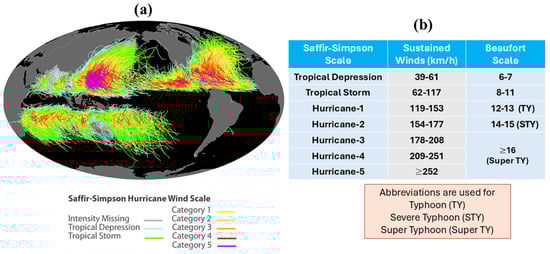
Figure 1. (a) Tracks of tropical cyclones recorded in years 1850–2018 using a colour scheme based on the Saffir–Simpson Hurricane Scale (www.ncei.noaa.gov/news/inventory-tropical-cyclone-tracks, accessed on 1 December 2025), and (b) sustained maximum wind speeds in terms of the Saffir–Simpson and Beaufort scales.

An overview is made in this paper on major research results made in the last 10 years using WCMS-NWA, with a special emphasis on (a) the performance of WCMS-NWA in simulating severe surface waves and ocean currents during extreme weather conditions and (b) quantifications of major contributions of WCIs. The structure of this paper is as follows. Section 2 and Section 3 describe the model setup and forcing of WCMS-NWA and assessment of model performances, respectively. Section 4 presents quantifications of WCIs based on results produced by WCMS-NWA. A summary and conclusions are given in Section 5.

2. Methodology

The advanced and coupled wave–current model known as WCMS-NWA has been used in simulating surface waves and 3D currents over the ECS and adjacent continental shelf and deep ocean waters under different weather conditions. WCMS-NWA has two versions. The first version was developed by Wang and Sheng [13] with the surface wave model known as SWAN [5] coupled to the 3D ocean circulation model known as the Princeton Ocean Model (POM) [16]. The current version of the coupled modelling system was developed by Lin et al. [14] with SWAN [5] coupled to ROMS [4]. Both POM and ROMS are free surface, terrain-following numerical models, which solve 3D Reynolds-averaged Navier–Stokes (RANS) equations using the hydrostatic and Boussinesq assumptions. Readers can refer to Wang and Sheng [13] and Lin et al. [14] for the setup and forcing specified in these two versions of the WCMS-NWA.

Since most of the model results to be discussed in this paper were generated by the current version of the WCMS-NWA, only a brief description of the current version is given here. The WCMS-NWA has two main sub-components: (a) the surface wave module based on SWAN (version 41.31) and (b) the 3D ocean circulation module based on ROMS (version 3.8), which are coupled using the Model Coupling Toolkit [17,18]. The domain of WCMS-NWA covers the eastern Canadian shelf and adjacent coastal and deep ocean waters between 80° W and 40° W and between 34° N and 55° N (Figure 2). The model bathymetry was extracted from the gridded bathymetric data known as the General Bathymetric Chart of the Oceans (www.gebco.net, accessed on 1 December 2025). The horizontal resolution of WCMS-NWA is 1/12° in longitude in both the eastward and northward directions. In the vertical direction, ROMS uses 40 vertical S-levels with higher vertical resolutions closer to the sea surface to resolve the 3D currents and hydrography in the upper ocean layers.

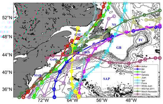
Figure 2. Domain and major topographic features of WCMS-NWA. Solid lines with different colours denote best tracks of 11 severe storms selected for this study. Abbreviations are used for the Labrador Shelf (LS), Newfoundland Shelf (NS), Gulf of St. Lawrence (GSL), Newfoundland (Nfld), Flemish Cap (FC), Grand Banks (GB), Scotian Shelf (ScS), Gulf of Maine (GoM), Middel Atlantic Bight (MAB), Slope Water (SW), and Sohm Abyssal Plain (SAP).

Wind stress and atmospheric pressures at the mean sea level (SLP) are important external model forcing particularly during severe weather conditions. Large-scale atmospheric forcing data were extracted from the fifth generation of the European Center for Medium-Range Weather Forecasts reanalysis (ERA5) [19]. During the passage of a storm within the model domain, high-resolution winds and SLP based on the Holland-type vortex model [20] or the Hurricane Wind Analysis System were blended into ERA5 for reliable representations of wind structures within the storm.

SWAN in the WCMS-NWA was driven by blended winds. Along the open boundaries of SWAN, the two-dimensional (2D) wave spectra were converted from the global WAVEWATCH III results provided by the National Oceanic and Atmospheric Administration (https://catalog.data.gov/dataset/wavewatch-iii-ww3-global-wave-model, accessed on 1 December 2025). The wave model (SWAN) was integrated in the spherical coordinates with a discrete spectrum consisting of 36 directions and 34 frequencies ranging from 0.04 to 1.0 Hz at a logarithmic increment of 0.1. The Discrete Interaction Approximation of Hasselmann et al. [21] was used for wave–wave interactions. The sea surface elevations and 3D currents produced by ROMS were used in SWAN. Effects of currents on waves (CEWs) specified in SWAN include (a) modification of wind speeds by currents (i.e., relative wind effect), (b) horizontal advection of surface waves and changes in the absolute frequencies of surface waves as a result of the Doppler shift, (c) current-induced wavenumber shift and wave refraction, and (d) modifications in the total water depth experienced by surface waves [22].

ROMS in the WCMS-NWA was also forced by the blended winds and SLP described above. The other atmospheric variables used in driving ROMS included shortwave radiation, long wave radiation, humidity, precipitation, air temperature, and cloud cover. Along the open boundaries of ROMS, both tidal forcing and non-tidal forcing were specified. The tidal forcing was extracted from the Oregon State University TOPEX/Poseidon Global Inverse Solution for barotropic tides (TPXO) [23] in terms of 11 tidal constituents (P₁, Q₁, O₁, K₁, M₂, S₂, N₂, K₂, M₄, MS₄, and MN₄). The non-tidal forcing at the open boundaries was specified in terms of daily mean currents and hydrography extracted from the Global Ocean Reanalysis and Simulation (GLORYS) [24]. Furthermore, freshwater discharges from 49 rivers within the model domain were specified using monthly mean climatology data from Environment and Climate Change Canada and U.S. Geological Survey, except for the St. Lawrence River. For this river, the monthly mean discharge values at Quebec City measured by the St. Lawrence Global Observatory were used. Readers can refer to Ohashi et al. [25] for additional information on specifications of river runoff and other details on model forcing.

Effects of surface waves on 3D currents (WECs) implemented in ROMS include four mechanisms: (i) wave-dependent wind stress [26], (ii) wave-enhanced mixing in the upper ocean [27], (iii) wave-enhanced bottom stress over coastal waters [28], and (iv) wave-induced forces on currents based on the vortex force formalism [22,29]. Detailed formulations of these four mechanisms can be found in Lin et al. [14].

For assessing model skills of WCMS-NWA and quantifying important contributions from WCIs, WCMS-NWA was applied to the study region during 11 selected storm events in the period 2003–2022 (Table 1). These 11 storms include 7 storms reaching hurricane strengths and 4 severe winter storms. They were highly severe storms significantly affecting the eastern Canadian shelf and adjacent waters during this 20-year period. The best tracks of these storms are shown in Figure 2. In the next section, we provide a review of our skill assessments of WCMs-NWA in simulating extreme ocean waves and currents during these severe weather events. For each storm, four numerical experiments were conducted using WCMS-NWA (Table 2), including (a) a fully coupled (FC) run, (b) wave-only (WO) run, (c) circulation-only (CO) run, and (d) smooth run (SR). In run FC, WCMS-NWA was integrated with two-way coupling between SWAN and ROMS. In run WO, only SWAN was integrated without using results from the circulation model. In run CO, only ROMS was integrated without using results from the surface wave model. In run SR, both SWAN and ROMS were driven by the smoothed atmospheric forcing in which storm effects were eliminated.

Table 1. List of 11 selected severe storms in the study region in years 2003–2022, with their maximum intensities, storm periods, and key references.

Index	Storm Name	Peak Intensity (Storm Period)	Key References
1	Hurricane Juan	Category-2 hurricane (Sep. 2003)	Wang et al. [12]
2	White Juan	Hurricane-strength winter storm (Feb. 2004)	Wang and Sheng [13]
3	Hurricane Bill	Category-1 hurricane (Sep. 2009)	Wang and Sheng [13]
4	Storm-A	Winter storm (Feb. 2011)	Lin et al. [30]
5	Hurricane Earl	Category-4 hurricane (Sep. 2010)	Lin et al. [14]
6	Hurricane Igor	Category-4 hurricane (Sep. 2010)	Lin et al. [14]
7	Hurricane Ophelia	Category-4 hurricane (Oct. 2011)	Lin et al. [30]
8	Storm-B	Winter storm (Mar. 2014)	Lin and Sheng [26]
9	Hurricane Arthur	Category-1 hurricane (June-July 2014)	Hughes et al. [15]
10	Storm Echo	Winter storm (Dec. 2015)	Wang and Sheng [31]
11	Hurricane Fiona	Category-4 hurricane (Sep. 2022)

Table 2. List of four model runs using the wave–current modelling system for the northwest Atlantic (WCMS-NWA).

Run	Case Description	Wave-Dependent Wind Stress	Wave-Induced Bottom Stress	Wave-Enhanced Vertical Mixing	Wave Forces
WO	Wave-Only Model Run	Off	Off	Off	Off
CO	Circulation-Only Model Run	Off	Off	Off	Off
FC	Fully Coupled Model Run	On	On	On	On
SR	Smoothed Atmospheric Forcing	On	On	On	On

3. Model Performance

Performances of WCMS-NWA were assessed using four statistical metrics [14], including (RB), root mean square error (RMSE), correlation coefficient (R), and γ² value. The last was suggested by Thompson and Sheng [32] for quantitative assessments of the model performance, given as

$${\gamma }^2={\displaystyle \frac{Var(X_o-X_m)}{Var\left(X_o\right)}}$$

(1)

where $X_m$ and $X_o$ represent, respectively, the simulated and observed value of variable X at the same observation time. The γ² values are in the range of 0 and infinity. Smaller γ² values imply better performances of the numerical model in simulating variable X. The critical value of γ² is set to 1.0 in this study.

Several studies were made in examining performances of WCMS-NWA in simulating surface waves and 3D currents during specific storm events [13,14,15]. In this overview, the feasibility and accuracy of WCMS-NWA in simulating extreme surface waves and intense ocean currents during the selected 11 storm events are considered. As shown in Figure 3 as an example, WCMS-NWA (early version) in run FC performed very well in reconstructing the observed large surface waves at four buoys generated by Hurricane Juan in late September 2003 [12]. In particular, WCMS-NWA reproduced very well the observed peak values of significant wave heights (SWHs, $H_s$) of about 8.8 m at buoy DWR (Figure 3a) and about 12.0 m at buoy 44142 (Figure 3b) on the left-hand side of the storm track. By comparison, WCMS-NWA slightly overestimated the observed peak values of SWHs to be about 9.0 m and 7.0 at buoys 44258 and 44137 (Figure 3d,e) on the right-hand side of the storm track. Without inclusion of CEWs, the model results in run WO also had overestimations on the right-hand side of the storm, and the overestimations in run WO were significantly larger than in run FC. The effects of near-inertial currents on the observed surface waves were also reproduced by WCMS-NWA in run FC (Figure 3a,b).

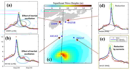
Figure 3. Time series of observed and simulated SWHs at buoys (a) WDR, (b) 44142, (d) 44258, and (e) 44137 during Hurricane Juan (September 2003). Positions of the four buoys are marked in (c). Blue (green) lines represent model results in run FC (WO). The black line with open circles in (c) represents the storm track of Hurricane Juan. Abbreviations are used for the right-hand side (RHS) and left-hand side (LHS) of the storm track. (Modified from Wang and Sheng [13] with permission of the American Geophysical Union).

Simulated SWHs ($H_s)$ and peak wave periods (PWPs, $T_p$) produced by WCMS-NWA in run FC were also found [14] to be in good agreement with observations during the passage of Hurricane Earl in September 2010 (Figure 4). During the passage of Hurricane Earl over the model domain in early September, WCMS-NWA performed very well in simulating the maximum values of observed SWHs of about 8.1 m at buoy 44008, 10.2 m at buoy 44137, and greater than 6.0 m at buoys 44141 and 44139 (Figure 4b). By comparison, the performance of WCMS-NWA was less satisfactory in reconstructing the observed PWPs at the six buoys during Hurricane Earl but still acceptable, particularly at buoys 44008, 44137, and 44255 (Figure 4c). The observed PWPs during Hurricane Earl occasionally shifted from longer values to shorter values. The observed shifts in PWPs were reproduced reasonably well by WCMS-NWA in run FC at buoy 44008 during 11–13 September, at buoy 44141 on 9 September, and at buoy 44255 on 21 September (Figure 4c). These PWP shifts were due to changes in wave spectra under the influence of currents.

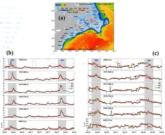
Figure 4. Time series of observed and simulated (b) SWHs ($H_s)$ and (c) PWPs ($T_p$) at buoys 44008, 44137, 44141, 44139, 44138, and 44020 in September 2010. The water depth at each buoy is shown in parentheses. Blue dashed (blue dotted) lines mark the peak SWHs during Hurricane Earl (Igor). Storm tracks of these two hurricanes and buoy locations are marked in (a), with the colour image representing water depth (m). (Modified from Lin et al. [14], with permission of the American Geophysical Union).

WCMS-NWA in run FC also performed reasonably well in reproducing the observed SWHs at the six buoy sites during the passage of Hurricane Igor in late September 2010 (Figure 4b). The maximum values of the observed and simulated SWHs generated by Hurricane Igor were about 12.0 m at buoy 44138; 9.0 m at buoys 44141 and 44139; and 7.5 m at buoy 44137, respectively (Figure 4b). WCMS-NWA in run FC performed reasonably well in simulating the observed PWPs during Hurricane Igor at buoys 44141, 44139, and 44138 but had large model deficiencies in simulating temporal shifts in observed PWPs at buoys 44008, 44137, and 44255 (Figure 4c). Although exact reasons are not known for these large model deficiencies at these sites, a possible explanation is large model errors in simulating upper ocean currents and associated variability over areas occupied by these three buoys.

Table 3 lists values of four error metrics for the simulated SWHs ($H_s)$ and PWP ($T_p$) at 16 buoy locations in September 2010 [14]. The positions of these buoys are marked in Figure 4a. Observations at buoy 44020 were not used since it was located in shallow waters off Nantucket Sound. The RB values are between –4.0% and 14.2% for SWHs and between –7.2% and 12.6% for PWPs at these 16 locations. The RMSE values are between 0.16 m and 0.40 m for SWHs and between 1.5 s and 2.9 s for PWPs. The R values are high and more than 84% for SWHs and moderately high and between 60% and 83%. The γ² values are very small and between 0.04 and 0.40 for SWHs and relatively large and between 0.31 and 0.72 for PWPs. There were similar values for these error metrics for the model results during Hurricane Juan in September 2003 (Figure 3). The statistical model error analyses reveal that WCMS-NWA has satisfactory skills in simulating SWHs and moderately satisfactory skills in simulating PWPs. It should be noted that relatively large model errors for PWPs are affected by many factors, including accuracy of wind forcing, parameterization for small-scale physical processes, initial and boundary conditions of the model, and difficulty in accurately resolving wave spectra [33].

Table 3. Summary of model error metrics for significant wave heights ($H_s$) and peak wave periods ($T_p$) at 17 buoys (marked in Figure 4a) in September 2010 [14]. The error metrics include the relative bias (RB), root mean square error (RMSE), correlation coefficients (R), and relative variance (${\gamma }^2$).

Buoy ID	Water Depth (m)	RB (%)		RMSE		R (%)		${\mathit{\gamma }}^2$
		${\mathit{H}}_{\mathit{s}}$	${\mathit{T}}_{\mathit{p}}$	${\mathit{H}}_{\mathit{s}}$ (cm)	${\mathit{T}}_{\mathit{p}}$ (s)	${\mathit{H}}_{\mathit{s}}$	${\mathit{T}}_{\mathit{p}}$	${\mathit{H}}_{\mathit{s}}$	${\mathit{T}}_{\mathit{p}}$
44007	27	16.9	6.6	24.0	2.2	87.1	71.5	0.40	0.40
44008	75	5.4	0.8	32.3	2.0	95.7	71.1	0.12	0.47
44009	43	−4.0	7.3	24.1	2.3	91.8	78.1	0.17	0.38
44013	64	0.0	12.6	13.8	2.9	85.8	61.1	0.29	0.49
44014	45	11.7	2.1	39.1	2.0	94.2	77.3	0.20	0.32
44017	48	0.0	1.4	26.1	1.8	93.1	82.6	0.12	0.23
44025	36	−3.9	3.8	26.0	2.2	90.6	78.8	0.20	0.31
44027	185	14.2	5.7	29.3	2.0	91.5	78.8	0.22	0.36
44137	4500	−0.3	−2.2	28.8	1.5	97.5	82.6	0.06	0.37
44138	1500	−4.2	−4.6	36.9	1.6	96.9	73.0	0.06	0.51
44139	1100	3.1	−5.4	24.9	2.0	98.3	70.6	0.04	0.58
44141	3000	1.7	−4.6	25.7	2.1	98.3	60.2	0.04	0.70
44150	1300	2.8	−1.6	28.7	2.0	97.4	71.4	0.05	0.57
44251	71	−2.0	−7.2	26.7	2.0	97.4	61.5	0.07	0.72
44255	179	0.1	−1.6	28.0	2.1	95.1	59.8	0.11	0.72
44258	60	−1.4	1.1	38.2	1.5	84.3	82.1	0.33	0.37

Model performances in simulating surface waves were also examined previously [14] using the directional 2D wave spectra observed at buoy 44008 during Hurricane Earl. At 05:00 on 4 September, large amounts of surface wave energy at this buoy were generated by peak winds of Hurricane Earl, with surface waves propagating nearly northward with wave frequencies of 0.06–0.10 Hz (Figure 5a). As Earl moved northward, the observed wave energy at this buoy became lower and broader with time. At 21:00 on the same day, the observed wave energy spread over the northwest and northeast directions with frequencies of 0.08–0.15 Hz (Figure 5d). In comparison with the observed wave spectra, WCMS-NWA in run FC performed reasonably well in reconstructing the observed directional spreads of 2D wave spectra (Figure 5b,d). It should be noted that there was less simulated directional spreading of the wave spectra than the observations, suggesting that further improvements in WCMS-NWA in simulating surface waves and directional spreading of 2D wave spectra are required.

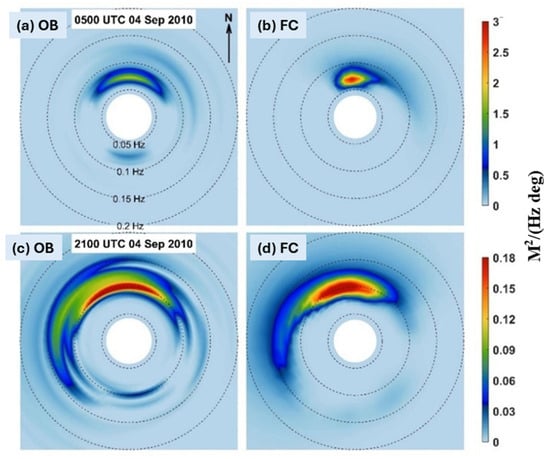
Figure 5. Distributions of (a,c) observed and (b,d) simulated 2D wave spectra at buoy 44008 at (a,b) 05:00 and (c,d) 21:00 on 4 September 2010 during the passage of Hurricane Earl. (Modified from Lin et al. [14], with permission of the American Geophysical Union).

Tidal sea levels and 3D tidal currents were simulated by WCMS-NWA with tidal forcing specified at the open boundaries of its circulation module. The satisfactory performance of WCMS-NWA in simulating tidal elevations and currents was presented in Pei et al. [34] using TPXO tidal elevations [23] and tidal results using the Nucleus for European Modelling of the Ocean (NEMO) [35]. As shown in Figure 6a,b, the co-amplitudes and co-phases of ${\mathrm{M}}_2$ tidal sea levels produced by WCMS-NWA agreed well with the TPXO tidal solution. In comparison with data-assimilative TPXO results, WCMS-NWA performed very well in generating large ${\mathrm{M}}_2$ amplitudes greater than 4.0 m in the Bay of Fundy and up to 1.5 m in the St. Lawrence Estuary. There were two M₂ amphidromic points over the study region, with one close to the eastern open boundary of the model domain and another in the central area of the Gulf of St. Lawrence. The M₂ tidal waves rotate cyclonically around each of the amphidromic points. As shown in Pei et al. [34], WCMS-NWA also performed well in simulating co-amplitudes and co-phases of ${\mathrm{K}}_1$ tidal sea levels.

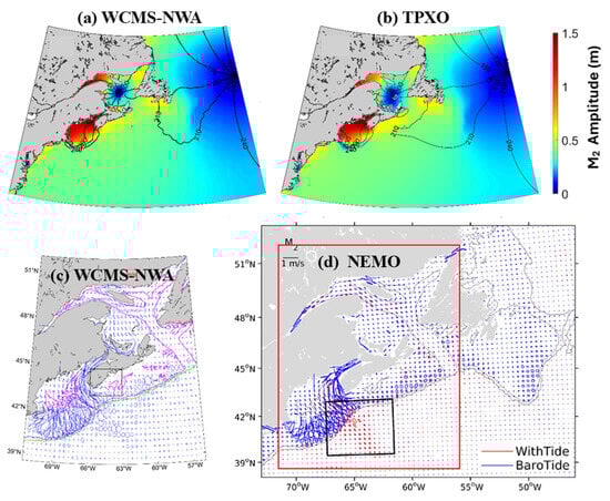
Figure 6. Distributions of co-amplitudes (image) and co-phases (contours) of ${\mathrm{M}}_2$ tidal sea levels produced by (a) WCMS-NWA and (b) TPXO. Tidal current ellipses of surface tidal currents produced by (c) WCMS-NWA and (d) NEMO. Magenta and green contours in (c) represent the 200 m and 1000 m isobaths, respectively. The red box in (d) marks the model domain of WCMS-NWA (Modified from Pei et al. [34]).

Figure 6c presents ellipses of ${\mathrm{M}}_2$ tidal currents at the surface computed from the 3D tidal currents produced by WCMS-NWA. The surface ${\mathrm{M}}_2$ tidal current ellipses had high spatial variability, with high tidal speeds (>1 m s⁻¹) in the Bay of Fundy and over the southern flank of Georges Bank and the southwestern Scotian Shelf [34]. The surface ${\mathrm{M}}_2$ current ellipses produced by WCMS-NWA were in a general agreement with their counterparts produced by NEMO over the domain of WCMS-NWA.

The satisfactory performance of WCMS-NWA in simulating total and tidal sea levels was established by comparing model results with in situ observations of sea levels at tidal gauges over the study region. As shown in Figure 7a–f, the time series of the total sea levels (${\eta }_T$) produced by WCMS-NWA in run FC agreed very well with the observed sea levels at six tide gauges in September 2014. During this period, the observed total sea levels at these locations (Figure 7g) were affected by winds and surface waves associated with Hurricane Arthur [15].

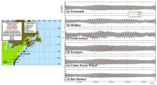
Figure 7. Time series of observed and simulated total sea levels (m) at tidal gauge stations of (a) Yarmouth, (b) Halifax, (c) North Sydney, (d) Eastport, (e) Cutler Farris Wharf, and (f) Bar Harbour during the period between 00:00 on 1 June 2014 and 06:00 on 10 July 2014. The storm track of Hurricane Arthur is shown in (g). (Modified from Hughes et al. [15]).

Table 4 lists values of three model error metrics for simulated total sea levels at 10 tidal gauges during the period from 1 June to 10 July 2014 [15]. The RMSE values are small and between 0.07 m and 0.46 m. The R values are very high and greater than 92%. The ${\gamma }^2$ values are very small and between 0.03 and 0.1. These indicate the satisfactory skills of WCMS-NWA in simulating the total sea levels during this period.

Table 4. Summary of model error metrics for the total sea levels at 10 tide gauge stations during the period between 1 June and 10 July 2014 [15].

Station	RMSE (cm)	R (%)	${\mathit{\gamma }}^2$
North Sydney	7.1	97.1	0.06
Halifax	8.0	98.7	0.03
Yarmouth	33.3	99.1	0.07
Eastport	46.2	92.2	0.06
Culter Farrie Wharf	27.8	98.5	0.03
Bar Harbour	28.5	97.8	0.06
Portland	30.0	96.5	0.09
Boston	31.6	96.0	0.10
Cape May	16.6	96.5	0.10
Duck	10.7	95.8	0.08

Both the observed and simulated total sea levels (${\eta }_T$) at North Sydney and Port aux Basques during Hurricane Fiona were decomposed into tidal (${\eta }_{tide}$) and non-tidal (${\eta }_{nt}$) components. These two tide gauges were located on the right-hand side of the storm track during this hurricane (Figure 8g). As shown in Figure 8a,d, the total sea levels produced by WCMS-NWA in run FC agreed well with the observations at these two tide gauges during this period, with ${\gamma }^2$ values less than 0.08. The simulated tidal sea levels (${\eta }_{tide}$) in run FC also agreed well with the observed tidal sea levels at these two locations (Figure 8b,e), with ${\gamma }^2$ values less than 0.05. WCMS-NWA in run FC also effectively reproduced the observed non-tidal sea levels at these two locations (Figure 8c,f), with ${\gamma }^2$ values less than 0.1. Note that the non-tidal sea levels can further be decomposed into the storm surge and contributions from WCIs.

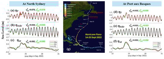
Figure 8. Time series of observed and simulated total, tidal, and non-tidal sea levels (m) at (a–c) North Sydney, (d–f) Port aux Basques during 22–31 September 2022. The storm track of Hurricane Fiona is shown in (g).

The skill of WCMS-NWA in simulating 3D hydrography over the NWA has been assessed in previous studies [13,14,15]. Figure 9 shows the observed and simulated daily mean sea surface temperatures (SSTs) over the model domain in September 2010. The observed SSTs were converted from satellite remote sensing data extracted from Remote Sensing Systems (RSS, www.remss.com, accessed on 1 November 2025).

Figure 9. Daily mean sea surface temperatures over the model domain computed from (a,c) satellite remote sensing data and (b,d) model results in run FC on (a,b) 6 and (c,d) 22 September 2010 during Hurricane Igor. (Modified from Lin et al. [14], with permission of the American Geophysical Union).

As shown in Figure 9a,b, the large-scale observed features of SSTs inferred from satellite data on 6 September 2010 were reproduced reasonably well by WCMS-NWA in run FC. The well-reproduced large-scale SST features included (a) warm (and high-salinity) surface waters carried by the Gulf Stream from shelf waters off Cape Hatteras to deep waters off the Grand Banks; (b) cold (and low-salinity) surface waters carried by the Labrador Current from the Labrador Sea southward through the Flemish Pass to the outer flank of Grand Banks; and (c) relatively cool (and low-salinity) surface waters of the eastern Canadian shelf including the Labrador Shelf, Newfound Shelf, Grand Banks, Gulf of St. Lawrence, Scotian Shelf, and Gulf of Maine. Due to intense vertical mixing generated by Hurricane Igor, the observed SSTs over the Grand Banks and Scotian Shelf on 22 September (Figure 9c) were significantly cooler than their counterparts on 6 September (Figure 9a). The significant surface cooling observed over the eastern Canadian shelf on this day (Figure 9c) was also well simulated by WCMS-NWA in run FC (Figure 9d). It should be noted that relatively large differences occurred in small-scale features (such as eddies and meanders) between the observed and simulated SSTs shown in Figure 9 due to the fact these small-scale hydrographic features were highly non-linear and accurate simulations of these small-scale circulation features required data assimilation.

One of important oceanographic features during the passage of a tropical storm (or hurricane) is a cool wake behind the storm [36,37,38]. This cool wake is generated mostly by intense vertical mixing induced by the storm (Figure 10). As shown in Wang and Sheng [13] and Lin et al. [14], WCMS-NWA has reasonable capabilities in simulating this storm-induced surface cooling along the storm wake. Figure 10 presents the observed and simulated differences ($∆\mathrm{S}\mathrm{S}\mathrm{T}$) between the post-storm and pre-storm SSTs in three storms, (a) Hurricanes Earl in September 2010, (b) Arthur in July 2014, and (c) Fiona in September 2022.

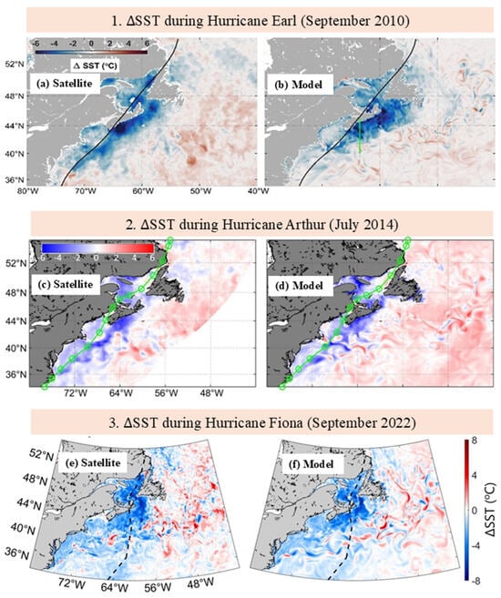
Figure 10. Storm-induced changes in sea surface temperatures ($∆\mathrm{S}\mathrm{S}\mathrm{T})$ during Hurricanes (a,b) Earl in September 2010, (c,d) Arthur in July 2014, and (e,f) Fiona in September 2022 calculated from (a,c,e) satellite observations and (b,d,f) on model results between runs FC and CO.

The observed fields of $∆\mathrm{S}\mathrm{S}\mathrm{T}$ during hurricane Earl in 2010 and Hurricane Arthur in 2014 (Figure 10a,c) were characterized by significant storm-induced surface cooling up to −6°C along the storm wake, with larger cooling on the right-hand side of the storm track than on the left-hand side, known as the rightward bias of storm-induced surface cooling [37]. The observed features of storm-induced surface cooling and rightward bias during these two hurricanes were well reproduced by WCMS-NWA (Figure 10b,d). During Hurricane Fiona in 2022, the observed $∆\mathrm{S}\mathrm{S}\mathrm{T}$ also featured significant surface cooling along the storm wake and rightward bias (Figure 10e). Furthermore, significant surface cooling also occurred over regions to the left-hand side of the storm track, including the western Gulf of St. Lawrence, Scotian Shelf, and Gulf of Maine during this storm. As shown in Figure 10f, WCMS-NWA also reproduced adequately the observed features of storm-induced $∆\mathrm{S}\mathrm{S}\mathrm{T}$ during hurricane Fiona. Readers can refer to previous studies [13,14,15] on the skill assessment of WCMS-NWA in simulating storm-induced hydrographic changes during storms.

We next summarize the capabilities of WCMS-NWA in simulating currents [15] by comparing simulated surface currents during Hurricane Arthur with observed currents inferred from high-frequency (HF) radar data archived by the Coastal Observing Research and Development Center (http://cordc.ucsd.edu/projects/mapping, accessed on 10 September 2025). At noon 4 July 2014, the centre of Hurricane Arthur reached the southern Middle Atlantic Bight (Figure 11a). Around the storm centre at this time, both the observed and simulated surface currents were very strong and cyclonic (counterclockwise), affected directly by the winds of Arthur. These cyclonic surface currents were highly asymmetric, with speeds of up to 1.0 m/s on the left-hand side of the storm and much stronger speeds of up to 2.0 m/s on the right-hand side of the storm. The intense northeastward surface currents over the right-rear quadrant of the storm to the east of Cape Hatteras were also affected by the Gulf Stream. Both the observed and simulated surface currents were weak over the northern Middle Atlantic Bight and relatively strong and cyclonic over southern New England. It should be noted that large differences occurred in current directions between the observed and simulated surface currents over southern New England, most likely due to less reliable wind forcing over this region at this time. Over the northern Gulf of Maine, WCMS-NWA performed very well in reproducing the observed surface currents forced mostly by tides at this time (Figure 11a).

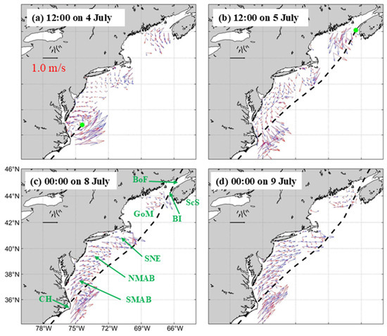
Figure 11. Comparisons between (blue) simulated surface currents in run FC and (red) observed surface currents inferred from HF radar data at (a) 12:00 on 4 July, (b) 12:00 on 5 July, (c) 00:00 on 8 July, and (d) 00:00 on 9 July during Hurricane Arthur in July 2014 (modified from Hughes et al., 2025 [15]). Abbreviations in (c) are used for the Bay of Fundy (BoF), Brier Island (BI), southern New England (SNE), northern Middle Atlantic Bight (NMAB), southern Middle Atlantic Bight (SMAB), north and Cape Hatteras (CH). (Modified from Hughes et al. [15]).

At noon on 5 July, Arthur reached Brier Island in southwestern Nova Scotia and downgraded to an extra-tropical cyclone (Figure 11b). The observed surface currents around the storm centre were also cyclonic at this time, with the maximum speed up to 1.0 m/s over the northern Gulf of Maine. WCMS-NWA in run FC reproduced the amplitudes of the observed surface currents over this area reasonably well but with relatively large model errors in current directions [15]. Although exact reasons are unknown for large model errors in current speeds, one of the plausible reasons is less accurate wind forcing over the coastal and shelf waters. Over the northern Gulf of Maine and Bay of Fundy, the surface currents were significantly affected by tidal currents. Both the observed and simulated surface currents at noon on 5 July were strong and southwestward over southern New England and relatively weak over the Middle Atlantic Bight. Over the offshore deep waters to the east of Cape Hatteras at this time, both the observed and simulated surface currents at this time were strong and northeastward, associated with the Gulf Stream (Figure 11b). The latter flowed northward over the continental slope of the eastern United States and separated abruptly from the continental shelf near Cape Hatteras to flow northeastward into the deep ocean waters of the Sohm Abyssal Plain.

The extra-tropical cyclone Arthur moved towards the Gulf of St. Lawrence on 6 July. During the post-storm period at 00:00 on 8 July (Figure 11c) and 00:00 on 9 July (Figure 11d), the observed surface currents were characterized by the intense northeastward Gulf Stream to the east of Cape Hatteras, and nearly spatially uniform and moderate northeastward currents over the Middle Atlantic Bight and southern New England. WCMS-NWA reproduced the observed surface currents reasonably well at these two times (Figure 11c,d).

Wang et al. [12] demonstrated good model capabilities in reconstructing the in situ observed currents made in a coastal embayment known as Lunenburg Bay of Nova Scotia during Hurricane Juan in September 2003. Readers can refer to their studies for more assessments of model performances in simulating observed currents in this bay.

4. Process Studies on Wave–Current Interactions

WCIs are non-linear processes in ocean dynamics where surface gravity waves and upper ocean currents exchange energy and momentum, which in turn modify both the surface waves and ocean currents [39,40]. Physically, WCIs can be separated into the current effects on waves (CEWs) and wave effects on currents (WECs) [13,41,42,43]. CEWs include (a) modifying effective wind speeds for generating surface waves at the sea surface, (b) modifying bottom stress experienced by waves at the sea bottom, (c) wave propagation and current-induced wave refraction, and (d) modifying wave frequency (Doppler shift). WECs include (i) modifying roughness height and surface stress and enhancing mixing by breaking waves at the sea surface, (ii) modifying bottom stress experienced by currents, (iii) additional momentum flux due to surface waves, and (iv) modifying vertical mixing by surface waves in the upper ocean.

Effects of WCIs during several severe storms over the study region were examined in our previous studies [13,14,15,44] based on model results produced by WCMS-NWA. In this section, important contributions from WCIs to surface waves and currents during hurricanes Juan, Bill, Arthur, and Fiona are summarized based on results produced by WCMS-NWA (Figure 12).

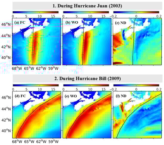
Figure 12. Swath maps of maximum SWHs ($H_s^{max}$) in (a,d) run FC and (b,e) in run WO, and (c,f) normalized differences (ND) in $H_s^{max}$ between runs FC and WO during Hurricanes (upper) Juan and (lower) Bill. The black line in each panel represents the storm track. (Modified from Wang and Sheng [13], with permission of the American Geophysical Union).

Figure 12a shows the swath maps of maximum SWHs ($H_s^{max})$ based on model results in run FC during the passage of Hurricane Juan in September 2003. The values of $H_s^{max}$ generated by this storm were considerably larger on the right-hand side of the storm track with the $H_s^{max}$ values up to 15 m and significantly smaller on the left-hand side. The rightward bias of maximum SWHs was associated with stronger winds and trapped wave resonance on the right-hand side than the counterparts on the left-hand side [13]. The trapped wave resonance can be explained by that the group velocity of the dominant swell waves (9–10 m/s) was very similar to the translation speed of Juan (9–15 m/s), so that surface waves on the right-hand side experienced a longer trapped fetch, resulting in larger $H_s^{max}$ than the counterparts on the left-hand side. As shown in Figure 12b, the maximum SWHs in run WO were also biased to the right-hand side of the storm track but with much larger magnitudes due to omission of CEWS in run WO. Figure 12c presents the relative differences in $H_s^{max}$ (${∆H}_s^{max}$) between runs FC and WO normalized by $H_s^{max}$ in run WO, indicating a significant reduction in $H_s^{max}$ (up to 15%) due to CEWS on the right-hand side of the hurricane track and a slight increase in $H_s^{max}$ (up to 7%) on the left-hand side. It was shown [13] that the relative wind effect and storm-generated strong surface currents are two important processes of CEWS responsible for large values of ${∆H}_s^{max}$ shown in Figure 12c.

During Hurricane Bill in September 2009, the simulated SWHs in run FC also had a remarkable rightward bias, with $H_s^{max}$ up to 15 m (Figure 12d). By ignoring CEWS, in comparison, the model results in run WO had large overestimations of $H_s^{max}$ on the right-hand side of the track (Figure 12e). The relative differences in $H_s^{max}$ between runs FC and WO (Figure 12f) also had a significant reduction in $H_s^{max}$ (up to 15%) due to CEWS on the right-hand side of Hurricane Bill [13].

As shown previously in Figure 3, the simulated SWHs during Hurricane Juan in run FC agreed better with the observations at four buoy sites than the model results in run WO [12], indicating the important contributions of CEWs. At buoys 44258 and 44137 on the right-hand side of the storm track (Figure 3d,e), the overestimations of $H_s^{max}$ in WO were significantly reduced by inclusion of CEWs in run FC. At buoys DWR and 44142 (Figure 3a,b) on the left-hand side of the storm track, modulations in the observed SWHs by near-inertial currents were well simulated by WCMS-NWA in run FC but not in run WO, suggesting again the importance of CEWs during Hurricane Juan. Similarly, during Hurricanes Earl and Igor in September 2010, the simulated SWHs and PWPs in run FC are in better agreements with observations at six buoy locations than the model results in run WO (Figure 4).

Effects of WECs on the upper-ocean hydrodynamics during extreme weather conditions including Hurricanes Juan (2003), Bill (2009), Earl (2010), and Igor (2010) were studied in the past [13,14]. Here, model results during Hurricane Fiona (2022) in three different runs (FC, CO, and SR in Table 3) are used to quantify the storm-induced changes in currents and hydrography and associated contributions of WECs to these changes.

The sea surface temperatures (SSTs) and currents (SSCs) during Hurricane Fiona in September 2022 produced by WCMS-NWA in run FC are shown in Figure 13. The general distributions of SST and SSS over the model domain during this period had warm and high-salinity surface waters carried by the Gulf Stream and cold and low-salinity surface waters carried by the equatorward Labrador Current. Over the coastal and shelf regions, the surface waters of the eastern Canadian shelf were also relatively cold and low-salinity. At 17:30 on 23 September (Figure 13a), the centre of Hurricane Fiona was located in the deep ocean waters near the southern open boundary. At this time, large storm-induced surface currents occurred over areas affected directly by the storm (i.e., AADS). Outside the AADS, large-scale SSCs and SSTs were not affected much by the storm. At 02:30 on 24 September, the storm centre reached the shelf break of the eastern Scotian Shelf (Figure 13b). SSCs over the AADS at this time were affected significantly by Hurricane Fiona, with intense near-inertial currents in the wake of the storm. The centre of Fiona moved to the southern Gulf of St. Lawrence (Figure 13c) by 20:30 on 24 September. The SSCs at this time featured intense wind-driven currents over the Gulf of St. Lawrence and eastern Scotian Shelf, and strong near-inertial currents in the wake of the storm. Over other regions, the SSCs had large-scale circulation features associated with the Gulf Stream and Labrador Current. At 00:30 on 26 September, Fiona moved to the LS and large storm-induced SSCs occurred in the wake of the storm (Figure 13d).

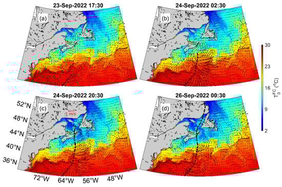
Figure 13. Distributions of sea surface temperature and currents produced by WCMS-NWA in run FC during the passage of Hurricane Fiona at (a) 17:30 on 23 September, (b) 02:30 on 24 September, (c) 20:30 on 24 September, and (d) 00:30 on 26 September 2022. The black line in each panel represents the storm track.

Differences in surface currents produced by WCMS-NWA between runs FC and SR were used to quantify the storm impacts on hydrodynamics during Hurricane Fiona. At 02:30 on 24 September, the storm-induced surface currents ($∆U^{ST}$) were large (up to 1.0 m/s) and cyclonic around the storm centre over the eastern ScS and also strong (up to 1.5 m/s) in the wake of the storm (Figure 14a). $∆U^{ST}$ were near-inertial in time with the large rightward bias. The $|∆U^{ST}|$ values were moderate (up to 0.4 m/s) over the Gulf of St. Lawrence, western Scotian Shelf, and Gulf of Marine, and relatively weak over regions far from the storm wake. At 00:30 on 26 September, the $|∆U^{ST}|$ values remained relatively large (up to in the storm wake, particularly in the deep ocean waters off the Scotian Shelf), and were relatively weak over regions far from the storm wake (Figure 14b).

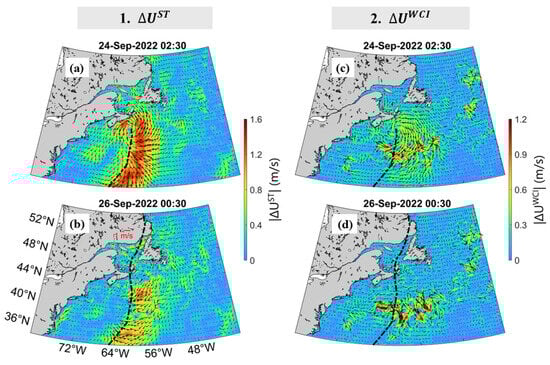
Figure 14. Distributions of (a,b) storm-induced surface currents ($∆U^{ST}$) based on differences between runs FC and SR and (c,d) WCI-induced surface currents ($∆U^{WCI}$) based on differences in surface currents between runs FC and CO at (a,c) 02:30 on 24 September and (b,d) 00:30 on 26 September 2022.

Contributions of WCIs to upper-ocean circulation during Hurricane Fiona were quantified using differences in currents ($∆U^{WCI}$) between runs FC and CO (Figure 14c,d). At 02:30 on 24 September, the WCI-induced surface currents ($∆U^{WCI}$) were large and up to 0.8 m/s and anti-cyclonic around the storm centre (Figure 14c). About 8.6 h after the storm’s passage, at 00:30 on 26 September, the |$∆U^{WCI}$| values were relatively small but not negligible in the storm wake (Figure 14d). This indicates the important role of WCIs in upper-ocean hydrodynamics during Hurricane Fiona.

Hydrographic distributions and vertical stratifications over the AADS during severe weather conditions were also affected significantly by WCIs [13,14]. The simulated SSTs produced by WCMS-NWA in run FC at 00:00 on 5 July and 00:00 on 7 July 2014 during the passage of Hurricane Arthur are shown in Figure 15a,b, respectively. The simulated SSTs at these two times featured relatively cold surface waters over the coastal and shelf waters of the eastern Canadian shelf and warmer surface waters along the path of the Gulf Stream. The WCI-induced changes in SSTs can be quantified using differences in SSTs between runs FC and CO ($∆{SST}^{FC-CO}$). The values of $∆{SST}^{FC-CO}$ are negative along the storm wake and coastal waters including the Grand Banks, Gulf of St. Lawrence, Scotian Shelf, and Gulf of Maine (Figure 15c,d). Relatively large positive and negative values of $∆{SST}^{FC-CO}$ also occur along the path of the Gulf Stream due to the high sensitivity of the eddies and meanders of the Gulf Stream [15].

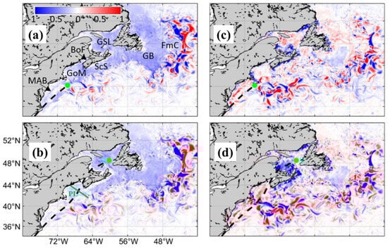
Figure 15. Distributions of (a,b) SST (°C) in run FC and (c,d) differences in SST between runs FC and CO ($∆{SST}^{FC-CO}$) at (upper) 00:00 on 5 July and (lower) 00:00 on 7 July 2014 during the passage of Hurricane Arthur.

Hydrography and vertical stratification beneath the sea surface were also modified by the storm and WCIs during Hurricane Arthur [15]. Figure 16a presents the vertical distribution of storm-induced temperature changes along transect PL (marked in Figure 15b). Over the near-shore section of transect PL (within 50 km from shore) where water depths are shallow, temperature changes induced by the storm were small due to the limited availability of sub-surface cold waters. Beyond this coastal section of the transect, a thin surface layer of storm-induced cooling extended seaward, with the maximum storm-induced surface cooling to be about −2.5 °C over the inner section of the transect and −3.0 °C over the middle section of the transect (Figure 16a). Below this thin cooling surface layer of less than 15 m, subsurface warming generated by the storm-induced vertical mixing occurred over the whole transect except for an area around 350 km and beyond 520 km from shore. The sub-surface waters with storm-induced warming of greater than 0.5 °C had the thickness of about 10–15 m over the inner section and about 20–80 m on the right-hand side of the track over the middle section of the transect. Over the outer section of the transect, two pools of storm-induced subsurface warming occurred at depths below 20 m.

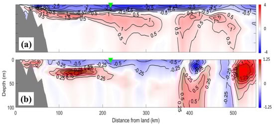
Figure 16. Vertical distributions of (a) storm-induced changes (post-storm minus pre-storm) in run FC and (b) two-day averaged WCI-induced changes in temperature ($∆T^{FC-CO}$) along the transect Penobscot Line (PL) during the passage of Hurricane Arthur in 2014. The green upside-down triangle symbol represents the location of the storm center of Hurricane Arthur.

Similarly, the WCI-induced temperature changes were quantified using differences in temperature between runs FC and CO $(∆T^{FC-CO})$. As shown in Figure 16b, WCIs led to noticeable temperature warming (up to 0.5 °C) over the near-shore section of transect PL. Beyond this near-shore section, WCI-induced temperature cooling (up to −0.5 °C) occurred in the surface layer at depths less than 20 m over the inner and middle sections of the transect. The WCIs generated large sub-surface warming (up to 1.0 °C) at depths between 20 m and 40 m over the inner section. Over the outer section of the transect beyond 370 km from shore, large values of $∆T^{FC-CO}$ extended from the surface to bottom, which were not induced by the WCIs but by cumulative WCI-induced changes over the two months leading up to Hurricane Arthur.

5. Discussion and Conclusions

A coupled wave–current modelling system for the northwestern Atlantic (NWA) was developed and calibrated by the Regional Modelling Group at Dalhousie University in the last 10 years. The NWA serves as an ideal study region due to its high storm frequency and intensity, offering a stringent testbed for coupled wave–current modelling. An incremental approach was taken in developing this advanced modelling system for the NWA known as WCMS-NWA, which has two versions. For the first version of WCMS-NWA, the three-dimensional (3D) circulation model known as POM was coupled to the third-generation spectral wave model known as SWAN using an external coupler [12]. This old version was used successfully to examine (a) representations of wave effects on 3D currents over coastal and shelf waters using the “vortex force” (VF) formulation and a “radiation stress” (RS) formulation [12], (b) semidiurnal tidal modulation in surface gravity waves [45], and (c) wave-induced vertical Reynolds stress [31]. For the second (and new) version of WCMS-NWA [14,46], the 3D circulation model known as ROMS was coupled to SWAN using the coupling toolkit in the COAWST platform [18]. The horizontal resolution of WCMS-NWA (current version) is 1/12° in longitude in both the eastward and northward directions, with 40 vertical S-levels in the vertical direction. New or modified parameterizations for different subgrid-scale processes such as depth-dependent wave breaking [14,26,30,46] and Langmuir turbulence [15] were incorporated incrementally into this new version.

Validation and calibration are very important for development and applications of any numerical ocean model. In this paper, performance of WCMS-NWA in simulating surface waves, ocean currents, and hydrography was discussed based on results and observations during 11 selected storms in the study region for the period 2003–2022. These 11 storms included 7 extreme storms with hurricane strength and 4 severe winter storms. These 11 storms spanned diverse scales and forcing intensities, enabling us to isolate and analyze how the coupled dynamics respond across a gradient of environmental conditions. WCMS-NWA was found to have excellent skills in simulating tidal elevations and tidal currents over the study region. It should be noted that tidal forcing was specified at the open boundaries of WCMS-NWA in terms of tidal elevations and depth-mean tidal currents converted from TPXO, without specifying the tide-generating potential forcing. Model performance in simulating tides can be further improved by including this tidal potential forcing as the body forcing [47]. WCMS-NWA also has satisfactory skills in simulating storm-induced surface elevations due partially to reliable representations of wind forcing associated with each storm in time and space by blending empirical winds calculated from the Holland-type vortex model [20] or high-resolution winds produced by the Hurricane Wind Analysis System into wind reanalysis such as ERA5. By comparing it with wave–buoy observations, WCMS-NWA was found to have very good capabilities in reproducing observed significant wave heights and was reasonably good at reproducing the observed peak wave periods during these 11 severe weather events. However, the simulated directional spreading of the wave spectra was found to be narrower than the observations, indicating that further improvements to WCMS-NWA are required.

Accurate simulations of 3D currents are significantly more challenging than accurate simulations of sea levels [48,49]. This is because 3D currents are affected by many factors including local topography, non-linear hydrodynamics, and wave–current–topography interactions, in addition to reliable representations of external forcing, reasonable model resolutions, and good parameterizations for subgrid-scale processes. Good agreement between simulated currents produced by WCMS-NWA with in situ and remote-sensing observations during 11 severe weather events reveal the satisfactory capabilities of the coupled wave–current model in simulating 3D circulation over the eastern Canadian shelf and adjacent waters. Wang and Sheng [13] showed satisfactory skills of WCMS-NWA with a nesting setup in simulating 3D currents observed in Lunenburg Bay in Nova Scotia during Hurricane Juan in September 2003. Hughes et al. [15] demonstrated, however, that WCMS-NWA had moderate capabilities in reproducing the amplitudes of surface currents converted from HF radar data but had large model errors in simulating current directions during Hurricane Arthur in July 2014. This indicates that further research is needed to improve the model’s capabilities in simulating 3D currents.

As shown in our recent studies, WCMS-NWA performed reasonably well in simulating large-scale features of temperature and salinity and storm-induced changes in hydrography over areas affected directly by the storm (AADS), without using data assimilation of in situ hydrographic observations and satellite observations. It should be noted that there were relatively large model errors in simulating small-scale features of observed hydrography associated with fronts, eddies, and meanders. These small-scale features are highly non-linear and their accurate simulation requires data assimilation. The other major weaknesses of WCMS-NWA include the lack of the a sea-ice modelling component and crude representations of subgrid-scale processes such as wave-induced mixing and unresolved internal waves.

The importance of having reliable representations of wave–current interactions (WCIs) was also augmented in this paper for accurate simulations of marine physical conditions [50], particularly during severe weather conditions. WCIs are highly non-linear processes where surface gravity waves and upper ocean currents exchange energy and momentum, which in turn modify both the surface waves and ocean currents. By taking advantage of the fully coupled nature between surface waves and ocean currents, model results produced by WCMS-NWA were used in examining (a) current effects on waves (CEWs) and (b) wave effects on currents (WECs) during 11 severe weather events. It was demonstrated that neglect of CEWs leads to significant overestimations of significant wave heights (SWHs) on the right-hand side of the storm track and underestimations of SWHs on the left-hand side on the North Hemisphere. Wang and Sheng [45] also demonstrated that surface wave variables (such as SWHs and PWPs) are modulated by semi-diurnal tidal currents in the Gulf of Maine, particularly around its mouth area, due to large effects of current-induced wave convergence, refraction, and wavenumber shift.

WCI-induced surface currents were found to be up to 1.0 m/s over the AADS, particularly on the right-hand side of the storm track (on the North Hemisphere). WCI-induced vertical mixing was also found to be very large in the surface mixed layer. As demonstrated in Wang and Sheng [12], a VF formulation with appropriate parameterization of wave breaking effects was able to produce reasonable results for applications in coastal and shelf waters during severe weather events. The RS formulation, by comparison, required a complex wave theory rather than a linear wave theory for the approximation of a vertical RS term to improve its performance under both breaking and nonbreaking wave conditions.

References

- Lighthill, J. Waves in Fluids; Cambridge University Press: Cambridge, UK, 2001; p. 205. ISBN 978-0-521-01045-0. [Google Scholar]
- Talley, L.; Pickard, G.; Emery, W.; Swift, J. Descriptive Physical Oceanography: An Introduction, 6th ed.; Elsevier: Boston, MA, USA, 2011; 560p. [Google Scholar]
- Dickey, T. Physical-optical-biological scales relevant to recruitment in large marine ecosystems. In Large Marine Ecosystems: Patterns, Processes, and Yields; Sherman, K., Alexander, L.M., Gold, B.D., Eds.; American Association for the Advancement of Science: Washington, DC, USA, 1990. [Google Scholar]
- Haidvogel, D.; Arango, H.; Hedstrom, K.; Beckmann, A.; Malanotte-Rizzoli, P.; Shchepetkin, A. Model evaluation experiments in the north Atlantic basin: Simulations in nonlinear terrain-following coordinates. Dyn. Atmos. Ocean. 2000, 32, 239–281. [Google Scholar] [CrossRef]
- Booij, N.; Ris, R.; Holthuijsen, L. A third-generation wave model for coastal regions: 1. Model description and validation. J. Geophys. Res. 1999, 104, 7649–7666. [Google Scholar] [CrossRef]
- Immas, A.; Do, N.; Alam, M. Real-time in situ prediction of ocean currents. Ocean Eng. 2021, 228, 108922. [Google Scholar] [CrossRef]
- Wang, X.; Jiang, H. Physics-guided deep learning for skillful wind-wave modeling. Sci. Adv. 2024, 10, eadr3559. [Google Scholar] [CrossRef] [PubMed]
- Mentaschi, L.; Vousdoukas, M.I.; García-Sánchez, G.; Fernández-Montblanc, T.; Roland, A.; Voukouvalas, E.; Federico, I.; Abdolali, A.; Zhang, Y.J.; Feyen, L. A global unstructured, coupled, high-resolution hindcast of waves and storm surge. Front. Mar. Sci. 2023, 10, 1233679. [Google Scholar] [CrossRef]
- Bagnasco, T.; Stocchino, A.; Vousdoukas, M.; Wang, J. A two-way coupled wave–current high resolution hindcast for the South China Sea. App. Ocean Res. 2025, 161, 104672. [Google Scholar] [CrossRef]
- Couvelard, X.; Lemarié, F.; Samson, G.; Redelsperger, J.; Ardhuin, F.; Benshila, R.; Madec, G. Development of a two-way-coupled ocean–wave model: Assessment on a global NEMO(v3.6)–WW3(v6.02) coupled configuration. Geosci. Model Dev. 2020, 13, 3067–3090. [Google Scholar] [CrossRef]
- Staneva, J.; Victor Alari, V.; Breivik, Ø.; Bidlot, J.; Mogensen, K. Effects of wave-induced forcing on a circulation model of the North Sea. Ocean Dyn. 2017, 67, 81–101. [Google Scholar] [CrossRef]
- Wang, P.; Sheng, J.; Hannah, C. Assessing the performance of formulations for nonlinear feedback of surface gravity waves on ocean currents over coastal waters. Cont. Shelf Res. 2017, 146, 102–117. [Google Scholar] [CrossRef]
- Wang, P.; Sheng, J. A comparative study of wave-current interactions over the eastern Canadian shelf under severe weather conditions. J. Geophys. Res. 2016, 121, 5252–5281. [Google Scholar] [CrossRef]
- Lin, S.; Sheng, J.; Ohashi, K.; Song, Q. Wave-current interactions during Hurricanes Earl and Igor in the northwest Atlantic. J. Geophys. Res. 2021, 126, e2021JC017609. [Google Scholar] [CrossRef]
- Hughes, C.J.; Sheng, J.; Perrie, W.; Liu, G. Performance assessment of the coupled circulation-wave modelling system for the northwest Atlantic. J. Mar. Sci. Eng. 2025, 13, 239. [Google Scholar] [CrossRef]
- Mellor, G. Users Guide for a Three Dimensional, Primitive Equation, Numerical Ocean Model; Program in Atmospheric and Oceanic Sciences, Princeton University: Princeton, NJ, USA, 2004. [Google Scholar]
- Larson, J.; Jacob, R.; Ong, E. The model coupling toolkit: A new Fortran90 toolkit for building multiphysics parallel coupled models. Int. J. High Perform. C 2005, 19, 277–292. [Google Scholar] [CrossRef]
- Warner, J.; Armstrong, B.; He, R.; Zambon, J. Development of a coupled ocean-atmosphere-wave-sediment transport (COAWST) modeling system. Ocean Modell. 2010, 35, 230–244. [Google Scholar] [CrossRef]
- Hersbach, H.; Bell, B.; Berrisford, P.; Hirahara, S.; Horányi, A.; Muñoz-Sabater, J.; Nicolas, J.; Peubey, C.; Radu, R.; Schepers, D.; et al. The ERA5 global reanalysis. Q. J. R. Meteorol. Soc. 2020, 123, 1–51. [Google Scholar] [CrossRef]
- Holland, G.J. An analytic model of the wind and pressure profiles in hurricanes. Mon. Weather Rev. 1980, 108, 1212–1218. [Google Scholar] [CrossRef]
- Hasselmann, S.; Hasselmann, K.; Allender, J.; Barnett, T. Computations and parameterizations of the non-linear energy transfer in a gravity-wave spectrum. Part II: Parameterizations of the non-linear energy transfer for application in wave models. J. Phys. Oceanogr. 1985, 15, 1378–1391. [Google Scholar] [CrossRef]
- Kumar, N.; Voulgaris, G.; Warner, J. Implementation and modification of a three-dimensional radiation stress formulation for surf zone and rip-current applications. Coast. Eng. 2011, 58, 1097–1117. [Google Scholar] [CrossRef]
- Egbert, G.; Erofeeva, S. Efficient inverse modelling of barotropic ocean tides. J. Atmos. Ocean. Technol. 2002, 19, 183–204. [Google Scholar] [CrossRef]
- Fernandez, E.; Lellouche, J. Product User Manual for the Global Ocean Physical Reanalysis Product GLOBAL_REANALYSIS_PHY_001_030; Report CMEMS-GLO-PUM, (001-030); EU Copernicus Marine Service: Toulouse, France, 2018; Volume 15. [Google Scholar]
- Ohashi, K.; Laurent, A.; Renkl, C.; Sheng, J.; Fennel, K.; Oliver, E. A coupled circulation-ice-biogeochemistry modelling system for the northwest Atlantic Ocean: Development and validation. Geosci. Model Dev. 2024, 17, 8697–8733. [Google Scholar] [CrossRef]
- Lin, S.; Sheng, J. Revisiting dependences of the drag coefficient at the sea surface on wind speed and sea state. Cont. Shelf. Res. 2020, 207, 104188. [Google Scholar] [CrossRef]
- Warner, J.; Sherwood, C.; Arango, H.; Signell, R. Performance of four turbulence closure models implemented using a generic length scale method. Ocean Model. 2005, 8, 81–113. [Google Scholar] [CrossRef]
- Madsen, O. Spectral wave-current bottom boundary layer flows. Coast. Eng. Proc. 1994, 1, 384–398. [Google Scholar]
- Uchiyama, Y.; McWilliams, J.; Shchepetkin, A. Wave-current interaction in an oceanic circulation model with a vortex-force formalism: Application to the surf zone. Ocean Model. 2010, 34, 16–35. [Google Scholar] [CrossRef]
- Lin, S.; Sheng, J.; Xing, J. Performance evaluation of parameterizations for wind input and wave dissipation in the spectral wave model for the northwest Atlantic Ocean. Atmos. Ocean. 2020, 58, 258–286. [Google Scholar] [CrossRef]
- Wang, P.; Sheng, J. Effects of wave-induced vertical Reynolds stress on upper-ocean momentum transfer over the Scotian Shelf during extreme weather events. Reg. Stud. Mar. Sci. 2020, 33, 100954. [Google Scholar] [CrossRef]
- Thompson, K.; Sheng, J. Subtidal circulation on the Scotian Shelf: Assessing the hindcast skills of a linear, barotropic model. J. Geophys. Res. 1997, 102, 24987–25003. [Google Scholar] [CrossRef]
- Cavaleri, L. Wave modeling—Missing the peaks. J. Phys. Oceanogr. 2009, 39, 2757–2778. [Google Scholar] [CrossRef]
- Pei, Q.; Sheng, J.; Ohashi, K. Numerical study of effects of winds and tides on monthly-mean circulation and hydrography over the southwestern Scotian Shelf. J. Mar. Sci. Eng. 2022, 10, 1706. [Google Scholar] [CrossRef]
- Madec, G. NEMO Reference Manual, Ocean Dynamics Component: NEMO-OPA; Note du Pole de modélisation; Institut Pierre-Simon Laplace (IPSL): Guyancourt, France, 2008; Volume 27. [Google Scholar]
- Price, J. Upper ocean response to a hurricane. J. Phys. Oceanogr. 1981, 11, 153–175. [Google Scholar] [CrossRef]
- Sheng, J.; Zhai, X.; Greatbatch, R. Numerical study of the storm-induced circulation on the Scotian Shelf during Hurricane Juan using a nested-grid ocean model. Prog. Oceanogr. 2006, 70, 233–254. [Google Scholar] [CrossRef]
- Zhang, H.; Liu, X.; Wu, R.; Chen, D.; Zhang, D.; Shang, X.; Wang, Y.; Song, X.; Jin, W.; Yu, L.; et al. Sea surface current response patterns to tropical cyclones. J. Mar. Syst. 2020, 208, 103345. [Google Scholar] [CrossRef]
- Cavaleri, L.; Fox-Kemper, B.; Hemer, M. Wind waves in the coupled climate system. Bull. Am. Meteorol. Soc. 2012, 93, 1651–1661. [Google Scholar] [CrossRef]
- McWilliams, J.; Restrepo, J.; Lane, E. An asymptotic theory for the interaction of waves and currents in coastal waters. J. Fluid Mech. 2004, 511, 135–178. [Google Scholar] [CrossRef]
- Craig, P.; Banner, M. Modeling wave-enhanced turbulence in the ocean surface layer. J. Phys. Oceanogr. 1994, 24, 2546–2559. [Google Scholar] [CrossRef]
- Bennis, A.; Ardhuin, F.; Dumas, F. On the coupling of wave and three-dimensional circulation models: Choice of theoretical framework, practical implementation and adiabatic tests. Ocean Model. 2011, 40, 260–272. [Google Scholar] [CrossRef]
- McWilliams, J.; Huckle, E.; Liang, J.; Sullivan, P. The wavy Ekman layer: Langmuir circulations, breaking waves, and Reynolds stress. J. Phys. Oceanogr. 2012, 42, 1793–1816. [Google Scholar] [CrossRef]
- Lin, S.; Sheng, J. Interactions between surface waves, tides, and storm-induced currents over shelf waters of the northwest Atlantic. J. Mar. Sci. Eng. 2023, 11, 555. [Google Scholar] [CrossRef]
- Wang, P.; Sheng, J. Tidal modulations of surface gravity waves in the Gulf of Maine. J. Phys. Oceanogr. 2018, 48, 2305–2323. [Google Scholar] [CrossRef]
- Lin, S.; Sheng, J. Assessing the performance of wave breaking parameterizations in shallow waters in spectral wave models. Ocean Model. 2017, 120, 41–59. [Google Scholar] [CrossRef]
- Wenzel, H. Tide-generating potential for the earth. In Tidal Phenomena; Wilhelm, H., Zürn, W., Wenzel, H., Eds.; Lecture Notes in Earth Sciences; Springer: Berlin/Heidelberg, Germany, 1997; Volume 66. [Google Scholar] [CrossRef]
- Fox-Kemper, B.; Adcroft, A.; Böning, C.W.; Chassignet, E.P.; Curchitser, E.; Danabasoglu, G.; Eden, C.; England, M.H.; Gerdes, R.; Greatbatch, R.J.; et al. Challenges and prospects in ocean circulation models. Front. Mar. Sci. 2019, 6, 65. [Google Scholar] [CrossRef]
- Causio, S.; Shirinov, S.; Federico, I.; Cillis, G.; Clementi, E.; Mentaschi, L.; Coppini, G. Coupling ocean currents and waves for seamless cross-scale modeling during Medicane Ianos. Ocean Sci. 2025, 21, 1105–1123. [Google Scholar] [CrossRef]
- Staneva, J.; Wahle, K.; Günther, H.; Stanev, E. Coupling of wave and circulation models in coastal–ocean predicting systems: A case study for the German Bight. Ocean Sci. 2016, 12, 797–806. [Google Scholar] [CrossRef]
Disclaimer/Publisher’s Note: The statements, opinions and data contained in all publications are solely those of the individual author(s) and contributor(s) and not of MDPI and/or the editor(s). MDPI and/or the editor(s) disclaim responsibility for any injury to people or property resulting from any ideas, methods, instructions or products referred to in the content. |
© 2025 by the authors. Licensee MDPI, Basel, Switzerland. This article is an open access article distributed under the terms and conditions of the Creative Commons Attribution (CC BY) license (https://creativecommons.org/licenses/by/4.0/).