Dynamic Mutual Adversarial Learning for Semi-Supervised Semantic Segmentation of Underwater Images with Limited and Noisy Annotations

Abstract

Swift and accurate semantic segmentation of underwater images is key for precise object recognition in complex underwater environments. Nonetheless, the inherent complexity of these environments and the limited availability of labeled data pose significant challenges to underwater image segmentation. Traditional deep learning methods struggle to cope with limited and noisy annotations. In this paper, we delineate the formulation of a novel semi-supervised paradigm with dynamic mutual adversarial training for the semantic segmentation of underwater images. This paradigm identifies the sources of inaccuracies in pseudo-labeling by analyzing different confidence maps, generated by models with unique prior knowledge. A dynamic reweighing loss function is then employed to orchestrate the mutual instruction of two divergent models. Furthermore, the delineation of confidence map is facilitated via adversarial networks, which involves simultaneous adversarial refinement of the discrimination network and the segmentation model, using the predictions with high-confidence maps as pseudo-labels. Experimental results on public underwater datasets verify that the proposed method can effectively improve semantic segmentation performance under the condition of a small amount of labeled data.

1. Introduction

Underwater environment perception, particularly optical visual perception, is crucial for the autonomous navigation and operation of underwater vehicles [1]. The timeliness and accuracy of semantic segmentation, a key technology in underwater perception, directly impact the overall performance of these systems. Therefore, efficient and precise semantic segmentation algorithms are essential for the practical application of intelligent sensing systems in underwater vehicles [2].

Deep neural networks, especially convolutional neural networks (CNNs), have recently shown great potential in the semantic segmentation of underwater images due to their excellent feature extraction and numerical regression capabilities [3,4]. However, most deep learning-based methods for underwater image segmentation require substantial amounts of labeled training data and precise pixel-wise labels for each image. The complex and unclear nature of underwater environments makes manual annotation labor-intensive and time-consuming, complicating the acquisition of large labeled datasets. To address this issue, semi-supervised semantic segmentation methods [5,6,7,8] have been proposed to reduce dependence on high-quality data by using self-/pseudo-supervision to perform segmentation without extensive manual labeling. Nonetheless, these methods often suffer from errors in pseudo labels. Previous self-training methods [9,10] always select pseudo labels based on confidence, derived from a model trained on a labeled subset. However, confidence-based methods have limitations: (1) to maintain a low error rate in pseudo labels, many low-confidence pseudo labels, which are naturally correct, are discarded; (2) errors in pseudo-supervision from the model itself (i.e., self-error) can significantly hinder semi-supervised learning performance.

To overcome the above challenges, we propose a novel semi-supervised method for semantic segmentation of underwater images, named Dynamic Mutual Adversarial Segmentation (DMAS). Our method employs a dual-model configuration where each model’s segmentations serve as checks for the other to enable the identification and correction of mislabeling. The key features of the DMAS methodology are as follows:

1.

The DMAS framework is based on two essential sub-processes: the first stage involves adversarial pre-training of two segmentation networks and their respective discriminators to develop two preliminary pseudo-label annotation models. The second stage is dynamic mutual learning, which measures the discrepancies between different segmentation models through confidence maps to mitigate the effects of potential pseudo label labeling errors, thereby enhancing the accuracy of the training process.

2.

The adversarial training method is mainly used for training a segmentation model and a fully convolutional discriminator with labeled data to generate pseudo-labels. This allows the discriminator to differentiate between real label maps and their predicted counterparts by generating a confidence map. Also, it enables a quantitative assessment of segmentation accuracy in specific regions of the pseudo-labels.

3.

Dynamic mutual learning guides different models based on their varying prior knowledge. It leverages the divergence between these models to detect inaccuracies in pseudo-label generation. By employing a dynamically reweighted loss function, it reflects the discrepancies between two models trained with each other’s pseudo-labels, thereby assigning lower weights to pixels with a higher likelihood of error.

4.

We validate the effectiveness of our proposed method on various underwater datasets, namely the DUT dataset and the SUIM dataset, demonstrating that the proposed semi-supervised learning algorithm is capable of enhancing the performance of models trained with limited and noisy annotations to be comparable to models supervised fully and trained with large amounts of labeled data.

2. Related Work

2.1. Pseudo-Label Methods for Semi-Supervised Semantic Segmentation

Pseudo-labeling [11,12] is a well-established technique in the domain of semi-supervised learning, with roots tracing back to some of the earliest works in the field [3]. Typically, pseudo-labeling based methods use models that have been trained on labeled datasets to predict provisional labels for unlabeled data. These predicted labels are then integrated into the existing dataset, which allows for the training of an improved model on this expanded dataset. Essentially, pseudo-labeling based methods can be divided into two categories: single-model based learning and mutual-model based learning.

Single-model based learning methods [13,14,15,16] rely on pseudo-labels generated by a single model within a self-training framework. However, these pseudo-labels are often unreliable since they rely solely on the prediction confidence of one model to filter out low-confidence labels. This strategy cannot detect and correct its labeling errors, which may result in the accumulation of bias and ultimately affect the training and segmentation effects.

To overcome this issue, mutual-model-based learning methods [17] have been proposed using multiple models obtained with different initial weight configurations or different portions of training data [18,19]. In this framework, each model iteratively retrains using pseudo-labels generated by other models rather than relying on its own predictions. This ensemble approach enhances the self-training mechanism, as each model supervises the others by providing pseudo-labels on unlabeled data, allowing for cross-supervision that helps identify and reduce errors in the pseudo-labels. Based on this methodology, we propose a dynamic mutual learning strategy that adjusts the learning weights assigned to each model through a dynamic allocation loss function, thereby improving the overall effectiveness and robustness of the learning process.

2.2. Adversarial Learning for Semi-Supervised Semantic Segmentation

Generative Adversarial Networks (GANs) [20], which comprise a generator and a discriminator, typically engage in a Min-Max game throughout the training process. This methodology has significantly contributed to the success of deep learning techniques in various image processing tasks [21,22], including semi-supervised semantic segmentation. Adversarial learning based semi-supervised semantic segmentation methods can be categorized into two distinct groups: generative and non-generative methods.

Generative methods [23,24] aim to extract and assimilate knowledge from a large corpus of unlabeled data and enhance the training dataset by generating new images. Essentially, a GAN consists of a generative component designed to mimic the distribution of the target image, thereby enabling the creation of new training examples. Simultaneously, the segmentation network acts as a discriminator, processing both real and artificially generated labels. However, since the generation method relies heavily on large volumes of unlabeled data, it can introduce significant distortion errors, leading to error accumulation.

Conversely, non-generative methods [25,26,27,28] replace the typical generative network of a classical GAN with a segmentation network. The output of this network is then fed to a discriminator that differentiates between real segmentation maps and those produced by the segmentation network. Zhang et al. [29] proposed an adaptive GAN-based segmentation algorithm aimed at improving the accuracy and generalizability of semi-supervised models. Fei et al. [30] integrated an attention mechanism into the semi-supervised learning framework for GANs, resulting in more precise predictions. Soul et al. [23] attempted to employ GANs for semi-supervised semantic segmentation, but their results were suboptimal due to significant deviations from authentic images. Luc et al. [31] introduced a training protocol for semantic segmentation using GANs that closely aligns with the framework discussed here. Inspired by above non-generative methods, we incorporated the adversarial learning to improve the evaluation of noise introduced during the pseudo-label generation stage, thereby reducing errors associated with pseudo-labels in a dynamic mutual learning context.

3. Methodology

3.1. Overview

Figure 1 illustrates our DMAS method, which comprises a two-stage training process: adversarial pre-training stage and dynamic mutual learning stage.

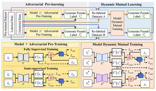
Figure 1. Overall framework of dynamic mutual adversarial segmentation (DMAS) method. The DMAS method consists of adversarial pre-training and dynamic mutual learning phases, enabling models A and B to exchange pseudo-supervision.

The adversarial pre-training stage uses a pre-training dataset divided into limited labeled data ${\mathcal{I}}_l$ and a larger set of unlabeled data ${\mathcal{I}}_u$ to develop two pre-trained segmentation networks $S^i(·),i\in \{A,B\}$ and a discriminator $D(·)$ capable of providing a quality evaluation, and to generate initial pseudo labels ${\widehat{y}}_{ps}^i$. This stage includes two steps: fully supervised training and semi-supervised training. Initially, the segmentation model $S^i(·)$ and the discriminator $D(·)$ are fully supervised using images $x_l\in {\mathcal{I}}_l$ and their corresponding labels $y_{gt}$, within a generative adversarial training framework where $S^i(·)$ acts as the generator. Then, using images $x_u\in {\mathcal{I}}_u$, the probability maps $D\left(S^i\left(x_u\right)\right)$ from the trained discriminator serves as a supervision signal for semi-supervised training of $S^i(·)$. High-probability outputs are selected as initial pseudo labels ${\widehat{y}}_{ps}^i$. We differentiate $S_A(·)$ and $S_B(·)$ by integrating prior knowledge from the ImageNet dataset into one of them.

In the dynamic mutual learning stage, the pre-trained segmentation networks $S^i(·),i\in \{A,B\}$ provide mutual supervision through dynamic self-training on re-labeled datasets. These datasets comprise initial labeled data ${\mathcal{I}}_l$, reliable pseudo-labeled data ${\mathcal{I}}_{ps}^i$, and remaining unlabeled data ${\mathcal{I}}_u^i$. Training involves using images $x_l^i\in {\mathcal{I}}_l\cup {\mathcal{I}}_{ps}^i$ and $x_u^i\in {\mathcal{I}}_u^i$, with labels $y_i\in {\mathcal{I}}_l\cup {\mathcal{I}}_{ps}^j$, and the probability map $D\left(S^i\left(x_u\right)\right)$ as supervision signals for $S^i(·)$. Pseudo labels ${\widehat{y}}_{ps}^i$ are then generated to update the pseudo-labeled data ${\mathcal{I}}_{ps}^j,j\in \{A,B\}$, $j\ne i$ and unlabeled data ${\mathcal{I}}_u^j$ of the other re-labeled dataset. A dynamic re-weighting loss $L_{DR}$ is introduced, utilizing the discrepancy between predicted confidence map and the discriminator-generated probability map $D\left(S^i\left(x_u\right)\right)$ to learn from the unlabeled data.

The purpose of this stage is to iteratively enhance the segmentation network models. The details on each component of our DMAS method will be described next.

3.2. Adversarial Pre-Training

The adversarial pre-training stage employs a Generative Adversarial Network (GAN) structure to enhance the quality of generated pseudo-labels, consisting of the segmentation network $S^i(·)$ and the discriminator $D(·)$. Subsequent pseudo-labels ${\widehat{y}}_{ps}^i$ are obtained by calculating probabilities through the discriminator on images generated by the segmentation network and selecting the top 10% of images. In this stage, both segmentation networks $S^i(·),i\in \{A,B\}$ and the discriminator $D(·)$ follow the same training process, which is divided into two steps: fully supervised training and semi-supervised training, as detailed in Algorithm 1.

Algorithm 1 Model Adversarial Pre-training.

Input: Labeled data ${\mathcal{I}}_l$; Unlabeled data ${\mathcal{I}}_u$ Output: Trained segmentation network $S(·)$; Trained discriminator $D(·)$     for number of fully supervised training iterations do        for $x_l\in {\mathcal{I}}_l,y_{gt}\in {\mathcal{I}}_l$ do            • Training steps:               1. Segmentation network training:                   $\mathrm{argmin}\left(L_{seg}(y_{gt},S\left(x_l\right))+{\lambda }_{pre}{L}_{pre}\left(D\left(S\left(x_l\right)\right)\right)\right)$               2. Discriminator training:                   $\mathrm{argmin}\left(L_{adv}(D\left(S\left(x_l\right)\right),D\left(y_{gt}\right))\right)$        end for      end for      for number of semi-supervised training iterations do        for $x_{all}\in {\mathcal{I}}_l\cup {\mathcal{I}}_u,x_u\in {\mathcal{I}}_u,x_l\in {\mathcal{I}}_l,y_{gt}\in {\mathcal{I}}_l$ do            • Segmentation network training:                $\mathrm{argmin}\left(L_{seg}(y_{gt},S\left(x_l\right))+{\lambda }_{pre}{L}_{pre}\left(D\left(S\left(x_{all}\right)\right)\right)+{\lambda }_{semi}{L}_{semi}\left(D\left(S\left(x_u\right)\right)\right)\right)$        end for      end for

3.2.1. Fully Supervised Training

In the fully supervised training step, the objective is to train the initial segmentation networks $S^i(·),i\in \{A,B\}$ and the evaluation-capable discriminator $D(·)$ using only labeled data ${\mathcal{I}}_l$. The labeled data includes images $x_l$ and their corresponding labels $y_{gt}$. We use the segmentation network $S^i(·)$ to predict segmentation results $S^i\left(x_l\right)$ from images $x_l\in {\mathcal{I}}_l$, which contain confidence information for each class. The discriminator $D(·)$ evaluates predicted results $S^i\left(x_l\right)$ with the corresponding probability maps $D\left(S^i\left(x_l\right)\right)$. To maintain the independence of the segmentation network and the discriminator, an alternating training strategy is employed: in each iteration, the segmentation network is trained while keeping the discriminator parameters fixed, and then the discriminator is trained while keeping the segmentation network parameters fixed. We use a multi-class segmentation loss function $L_{seg}(y_{gt},S\left(x_l\right))$ and a prediction loss function ${\lambda }_{pre}{L}_{pre}\left(D\left(S\left(x_l\right)\right)\right)$ to optimize the segmentation network $S^i(·)$ to deceive the discriminator; the adversarial loss $L_{\mathrm{adv}}$ is used to optimize the discriminator $D(·)$ to detect subtle differences between predicted segmentation images and true labels. After fully supervised training, the segmentation network attains initial segmentation capability, and the discriminator acquires the ability to evaluate the reliability of predicted segmentation images.

3.2.2. Semi-Supervised Training

In the semi-supervised training step, the model’s performance is further enhanced using unlabeled data ${\mathcal{I}}_u$. The discriminator, which is proficient at distinguishing predictions from the segmentation network, generates probability maps that can act as a supervisory signal to identify areas consistent with the true label distribution. A threshold is applied to convert this map into a binary format, highlighting regions of high confidence. These regions, now serving as pseudo-labels, facilitate the self-training of the model, with the most effective iteration being determined through comparative evaluation against previous iterations. The semi-supervised training step focuses on minimizing the semi-supervised loss $L_s$ while keeping the discriminator’s parameters fixed:

$$\begin{array}{c}\hfill L_s=L_{seg}+{\lambda }_{pre}{L}_{pre}+{\lambda }_{semi}{L}_{semi}\end{array}$$

(1)

where $L_{seg}$ and $L_{pre}$ are the multi-class segmentation loss function and the prediction loss function, respectively, and $L_{semi}$ represents the semi-supervised multi-class cross-entropy loss. The hyperparameters ${\lambda }_{pre}$ and ${\lambda }_{semi}$ are used to balance the weights of the terms. $L_{seg}$ and $L_{pre}$ are the same as in supervised training. The semi-supervised cross-entropy loss $L_{semi}$ is defined as

$$\begin{array}{c}\hfill L_{semi}=-\sum _{h,w}\sum _{c\in C}I(D\left(S\left(x_u\right)\right)>T_{semi})·mlog\left(S\left(x_u\right)\right)\end{array}$$

(2)

where $I(·)$ is the indicator function for high-probability pixel classification, while $T_{semi}$ is the threshold that controls the sensitivity of the semi-supervised process. By binarizing the probability map $D\left(S\left(x_u\right)\right)$, we can balance the credibility of generated pseudo-labels against the amount of data; specifically, a larger threshold $T_{semi}$ can increase the credibility of the pseudo-labels, but the number of usable pseudo-labels will decrease accordingly. To enhance the utilization of unlabeled data, we set $T_{semi}=0.2$. Since $S\left(x_u\right)$ employs one-hot encoding, we set $m^{(h,w,c)}$ to control category input. Therefore, when $c^{*}=\underset{c}{argmax}S{\left(x_u\right)}^{(h,w,c)}$, it follows that $m^{(h,w,c^{*})}=1$; otherwise, $m^{(h,w,c^{*})}=0$.

The confidence map serves as a pixel-level reliability filter in the adversarial pre-training stage, directly linking the discriminator’s probability evaluation to pseudo-label refinement. Its generation strictly follows the GAN interaction logic between the generator $S^i(·)$ and discriminator $D(·)$, and complies with established threshold and function definitions. After fully supervised training, the discriminator outputs a pixel-wise probability map for any input image. Each pixel value in this map represents the similarity between the corresponding segmentation result and real label maps—a higher value indicates lower prediction error risk. This probability map undergoes pixel-wise normalization and is used directly as the raw input for confidence map generation, with no additional processing required. To convert the continuous probability map into a binary reliability indicator, a threshold $T_{semi}=0.2$ and an indicator function are adopted. The confidence map pixel value for an unlabeled image is defined as the output of the indicator function. A value of 1 denotes a high-confidence pixel (reliable for pseudo-labels), while a value of 0 denotes a low-confidence pixel (excluded from pseudo-labeling). This balances data utilization—retaining sufficient pixels via $T_{semi}=0.2$—and pseudo-label quality—filtering high-error regions. Functionally, the confidence map refines pseudo-label selection by retaining only high-confidence pixels within the “top 10% images” to form ${\widehat{y}}_{ps}^i$, reducing pseudo-label noise compared to image-level selection. It also implicitly constrains the semi-supervised loss in the training loop, with only high-confidence pixels contributing to loss calculation, preventing low-confidence prediction errors from misleading model training.

3.3. Dynamic Mutual Learning

As depicted in Figure 1, during the Dynamic Mutual Learning (DML) stage, the segmentation network parameters are progressively refined through iterative updates of the dynamic mutual learning algorithm applied to the re-labeled datasets A and B. Dataset $i\in \{A,B\}$ consists of four components: (1) initial labeled data ${\mathcal{I}}_l$; (2) re-labeled pseudo-labeled data ${\mathcal{I}}_{ps}^i$ generated by the model itself in previous iterations; (3) cross-supervised pseudo-labels ${\widehat{y}}_{ps}^j$ iteratively updated from the other model $S^j(·)$ ($j\in \{A,B\},j\ne i$); (4) remaining unlabeled data ${\mathcal{I}}_u^i$ (after excluding samples used for ${\mathcal{I}}_{ps}^i$). This composition aligns with the two-stage workflow of Figure 1, where Dataset A and B, respectively, correspond to the “Re-labeled Datasets A/B” output from the adversarial pre-training stage and participate in mutual training between Model A and B. Dataset $i\in \{A,B\}$ consists of initial labeled data ${\mathcal{I}}_l$, re-labeled data ${\mathcal{I}}_{ps}^i$, data iteratively updated from the other model $S^j(·)$ ($j\in \{A,B\},j\ne i$), and its corresponding reduced unlabeled data ${\mathcal{I}}_u^i$. By analyzing the unlabeled images $x_u^i\in {\mathcal{I}}_u^i$, labeled images $x_l^i\in {\mathcal{I}}_l\cup {\mathcal{I}}_{ps}^i$, and corresponding labels $y_i\in {\mathcal{I}}_l\cup {\mathcal{I}}_{ps}^i$, the models iteratively update, leveraging differences to detect errors in automatically generated pseudo labels. Here, differences specifically refer to inter-model divergence between $S^i$ and $S^j$, which addresses the key limitation of single-model self-training where self-generated errors cannot be corrected—this is a core design of DML that Figure 1 visually reflects through the Mutual Training module connecting Model A and B. Additionally, a dynamic reweighting loss $L_{DR}$ is introduced to account for the discrepancies between the two models. Each model $S^i(·)$ is trained using pseudo labels ${\widehat{y}}_{ps}^j$ generated by the other model $S^j(·)$; thus, greater pixel-level discrepancies suggest higher error likelihoods and require reduced weighting in the loss function. This minimizes the impact of those pixels or regions with significant differences on the training process. The subsequent section details the dynamic mutual iterative framework and the dynamic reweighting loss.

3.3.1. Dynamic Mutual Iterative Framework

The dynamic mutual iteration framework employs an iterative learning model that progresses from simple to complex tasks. It involves repeatedly executing a “mutual training” algorithm over multiple cycles, where Model A and Model B alternately generate high-confidence pseudo labels for each other and update parameters using the dynamic reweighting loss. Effectively utilizing cross-supervised pseudo labels is crucial for enhancing the use of unlabeled datasets. This framework is consistent with Algorithm 1 and extends it to dual-model mutual optimization, as detailed in Algorithm 2.

Algorithm 2 Dynamic Mutual Learning (DML).

Input: Pre-trained models $S^A(·),S^B(·)$ (from adversarial pre-training); Re-labeled Dataset A (${\mathcal{I}}_l,{\mathcal{I}}_{ps}^A,{\mathcal{I}}_u^A$), Dataset B (${\mathcal{I}}_l,{\mathcal{I}}_{ps}^B,{\mathcal{I}}_u^B$); Discriminator $D(·)$; Hyperparameters ${\lambda }_{DR}$ Output: Final trained models $S^A(·),S^B(·)$     for number of DML iterations do        • Step 1: Generate cross-supervised pseudo-labels from $S^A(·)$  for Dataset B        for $x_u^B\in {\mathcal{I}}_u^B$ do          Generate pseudo-label and update ${\mathcal{I}}_{ps}^B$: ${\widehat{y}}_{ps}^A=S^A\left(x_u^B\right)$          Compute confidence map: $C^A=D\left(S^A\left(x_u^B\right)\right)$        end for       • Step 2: Update $S^B(·)$ using $S^A(·)$’s pseudo-labels and $L_{DR}$        for $x_l^B\in {\mathcal{I}}_l\cup {\mathcal{I}}_{ps}^B,x_u^B\in {\mathcal{I}}_u^B,y_{gt}\in {\mathcal{I}}_l\cup {\mathcal{I}}_{ps}^B$ do            Predict with $S^B(·)$: ${\widehat{y}}_{ps}^B=S^B\left(x_u^B\right)$            Compute confidence map: $C^B=D\left(S^B\left(x_u^B\right)\right)$            Update $S^B(·)$: $\mathrm{argmin}(L_s(y_{gt},S^B\left(x_l^B\right))+L_{DR})$        end for      • Step 3: Generate cross-supervised pseudo-labels from $S^B(·)$ for Dataset A (symmetric to Step 1)        for $x_u^A\in {\mathcal{I}}_u^A$ do            Generate pseudo-label and update ${\mathcal{I}}_{ps}^A$: ${\widehat{y}}_{ps}^B=S^B\left(x_u^A\right)$            Compute confidence map: $C^B=D\left(S^B\left(x_u^A\right)\right)$        end for        • Step 4: Update $S^A(·)$ using $S^B(·)$’s pseudo-labels and $L_{DR}$ (symmetric to Step 2)        for $x_l^A\in {\mathcal{I}}_l\cup {\mathcal{I}}_{ps}^A,x_u^A\in {\mathcal{I}}_u^A,y_{gt}\in {\mathcal{I}}_l\cup {\mathcal{I}}_{ps}^A$ do            Predict with $S^A(·)$: ${\widehat{y}}_{ps}^A=S^A\left(x_u^A\right)$            Compute confidence map: $C^A=D\left(S^A\left(x_u^A\right)\right)$            Update $S^A(·)$: $\mathrm{argmin}(L_s(y_{gt},S^A\left(x_l^A\right))+L_{DR})$        end for    end for

Algorithm 2 explicitly reflects the dual-model mutual optimization logic of DML: Steps 1–2 complete the update of $S^B(·)$ using pseudo-labels from $S^A(·)$, while Steps 3–4 symmetrically update $S^A(·)$ using pseudo-labels from $S^B(·)$. This closed-loop iteration ensures that both models continuously correct each other’s pseudo-label errors via inter-model divergence. During each update, the dynamic reweighting loss $L_{DR}$ is combined with the semi-supervised loss $L_s$ to suppress the impact of high-error pixels, aligning with the loss combination rule $L=L_s+L_{DR}$.

3.3.2. Dynamic Reweighting Loss

We introduce the dynamic reweighting loss with inter-model disagreement as reweighting weight. Assuming segmentation model $S^A(·)$ is used to train segmentation model $S^B(·)$, let $x_u^A$ represent the unlabeled images from unlabeled data ${\mathcal{I}}_u^A$. We define its pseudo label as ${\widehat{y}}_{ps}^{A(h,w,c)}=S^A{\left(x_u^A\right)}^{(h,w,c)}$, with ${C^A}^{(h,w)}=D{\left(S^A\left(x_u^A\right)\right)}^{(h,w)}$ being the probability map. Similarly, ${\widehat{y}}_{ps}^{B^{(h,w,c)}}=S^B{\left(x_u^A\right)}^{(h,w,c)}$ is the prediction during training, with $C^B(h,w)=D{\left(S^B\left(x_u^A\right)\right)}^{(h,w)}$ as the probability map. In the loop iteration of training the segmentation model $S^A(·)$, let ${p^B}^{(h,w,c)}={\widehat{y}}_{ps}^{B^{(h,w,c)}}·{C^B}^{(h,w)}$ represent the confidence-weighted predicted probability of class c by $S^B(·)$, integrating both the model’s prediction result and the discriminator’s reliability assessment. This is the $p_B$ referenced in the definition of weight ${\omega }_u^{(h,w)}$, which quantifies the credibility of $S^B(·)$’s prediction at each pixel. The dynamic reweighting loss weight ${\omega }_u^{(h,w)}$ is defined as

$$\begin{array}{c}\hfill {\omega }_u^{(h,w)}=\left\{\begin{array}{c}{p}_B,\mathrm{if}{\widehat{y}}_{ps}^A={\widehat{y}}_{ps}^B\hfill \\ p_B,\mathrm{if}{\widehat{y}}_{ps}^A\ne {\widehat{y}}_{ps}^B\mathrm{and}{C}^A\ge C^B\hfill \\ 0,\mathrm{if}{\widehat{y}}_{ps}^A\ne {\widehat{y}}_{ps}^B\mathrm{and}{C}^A\le C^B\hfill \end{array}\right.\end{array}$$

(3)

The dynamic reweighting loss on unlabeled samples, $L_{DR}$, is then defined as

$$\begin{array}{c}\hfill L_{DR}=-\sum _{h,w}{\omega }_u^{(h,w)}\sum _{c\in C}{\widehat{y}}_{ps}^{A(h,w,c)}log\left({\widehat{y}}_{ps}^{B(h,w,c)}\right)\end{array}$$

(4)

In the loop iteration of training the segmentation model $S^B(·)$, $L_{DR}$ is calculated using the same method, except that the results of the two segmentation models are swapped in order.

4. Experiments

4.1. Dataset

To evaluate the effectiveness of the proposed Dynamic Mutual Adversarial Segmentation (DMAS), we conducted experiments on two publicly available underwater datasets: DUT and SUIM. The DUT dataset includes 6617 images, of which 1487 images have semantic segmentation and instance segmentation annotations, and the remaining 5130 images have object detection box annotations, categorized into four classes: starfish, holothurian, scallops, and echinus. The SUIM dataset includes 1525 images for training and validation, along with 110 test images, each with pixel-level annotations. It encompasses eight categories: fish (FS), reefs (RF), aquatic plants (PL), wrecks/ruins (WR), human divers (DR), underwater robots (RB), and seafloor (SF). Both datasets are divided into training and testing datasets in a 7:3 ratio.

In the training set, we partitioned the labeled and unlabeled data using varying labeled ratios (0.5, 0.25, 0.125, and 1). Specifically, at each random shuffle of the entire training set, the first 0.5, 0.25, and 0.125 fractions were used as labeled data. When the labeled ratio is set to 1, it denotes fully supervised learning, involving only the training and testing sets. To verify the method’s adaptability to noisy annotations, label noise including partial label missing and incomplete labels was randomly introduced into the training set.

4.2. Implementation Details

The proposed method was implemented using PyTorch 1.12.1. The evaluation was conducted on a server equipped with an Intel Xeon(R) Silver 4214R CPU and an NVIDIA RTX A6000 48GB GPU. We utilized DeepLabv3 with ResNet-101 [32] as the backbone. The entire model was trained for 40,000 iterations, saving the model every 200 iterations during the dynamic mutual learning. The optimal model was selected based on predictions on the test set.

For pre-training, the initial learning rate was set to 0.001, with a weight decay of ${10}^{-4}$. The discriminator was trained using the Adam optimizer with a learning rate of ${10}^{-4}$. For hyperparameters in the SUISS method, we set them to 0.01 and 0.001 when using labeled and unlabeled data, respectively. Random cropping, random mirroring, and other data augmentation techniques were applied to mitigate overfitting and enhance model performance. To ensure the difference between Model A and Model B, all experiments below show that Model A is an untrained network, while Model B is a pre-trained network using the ImageNet dataset.

4.3. Evaluation Metrics

To objectively evaluate and analyze the performance of the DMAS method, we used the mean Pixel Accuracy (m)

$$\begin{array}{c}\hfill PA={\displaystyle \frac{TP+TN}{FN+FP+TP+TN}}\end{array}$$

(5)

IoU indicates the intersection over the union between the predicted and the actual value for each category. mIoU is the average IoU across all categories, and its calculation is shown:

$$\begin{array}{c}\hfill mIoU={\displaystyle \frac{1}{k+1}}\sum _{i=0}^{k}IoU={\displaystyle \frac{1}{k+1}}\sum _{i=0}^k{\displaystyle \frac{TP}{FN+FP+TP}}\end{array}$$

(6)

4.4. Performance Comparison

We compared the DMAS method on the DUT and SUIM datasets with several widely used fully supervised semantic segmentation algorithms, including the following:

(a) Supervised learning with fine tuning: FCN [33], DeeplabV3 [23] and LR-ASPP [34] methods.

(b) Semi-supervised learning: CutMix augmentation [35] and hybrid method s4GAN+MLMT [36].

All the above algorithms were implemented on the PyTorch platform, utilizing the same NVIDIA RTX A6000 48GB GPU, and were evaluated using the same pre-training and parameters on both the DUT and SUIM datasets.

4.4.1. Quantitative Analysis

Figure 2 display the differential outcomes of semantic segmentation experiments conducted at varying labeled ratios on the DUT and SUIM datasets, respectively. Analyzing these tables reveals that our proposed method, DMAS, exhibits superior performance compared to existing supervised and semi-supervised learning approaches, even with limited data availability in the DUT and SUIM datasets. Notably, DMAS maintains a consistently high performance regardless of reduced training sample sizes with label noise. For instance, at a labeled ratio of 0.125 with noise, DMAS still achieves mIoU and mPA metrics comparable to those of fully supervised methods without noise, confirming its robustness to both sparse and noisy labels. These results highlight the robustness and effectiveness of DMAS in handling scenarios with sparse labeled data. The data clearly support the hypothesis that the semi-supervised DMAS algorithm provides a significant advantage in semantic segmentation tasks, particularly when labeled ratios are limited, thus establishing its superiority in data-efficient learning models.

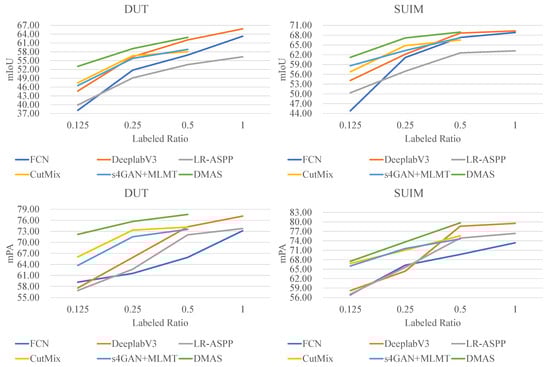
Figure 2. Comparative experimental results under different labeled ratios on DUT dataset and SUIM dataset. DMAS excels in semantic segmentation with 0.125 labeled ratio data, proving its robustness and data efficiency.

4.4.2. Qualitative Analysis

To provide a more tangible evaluation of DMAS’s performance, we conducted training on the DUT and SUIM datasets with an annotation ratio of 0.125. The comparative results are illustrated in Figure 3 and Figure 4. It is apparent that, even with a limited number of annotated samples, the DMAS method significantly outperforms other semantic segmentation methods based on full supervision or semi-supervision, particularly in terms of pixel classification accuracy and object boundary delineation. Specifically, as shown in the fifth row of Figure 3 and the third column of Figure 4, when various methods segment the same image, DMAS demonstrates superior performance in contour edge articulation, pixel classification over larger areas, and the accuracy of classification for smaller objects, surpassing other methods. This reflects DMAS’s efficacy in leveraging unlabeled data to enhance the model’s segmentation capability, thereby achieving successful semi-supervised learning. However, there remains a noticeable gap between DMAS’s predictions and the actual labels, as illustrated in the first row of Figure 3 and the thirteenth row of Figure 4. The precision of edge segmentation and regional delineation for targets is still suboptimal, which may be due to inherent performance limitations of the segmentation network or an insufficiency of training data. Specifically, for concealed targets (starfish obscured by aquatic plants in the first row of Figure 3, human divers hidden behind reefs in the tenth row of Figure 4), DMAS only achieves relatively low coverage of occluded regions. This is attributed to feature overlap between occluders and targets, which causes the discriminator D to generate probability maps with low confidence, leading the dynamic reweighting loss $L_{DR}$ to excessively downweight valid pixels and suppress the learning of occluded target features. For low-contrast targets (e.g., in Figure 4), the boundary pixel error rate is relatively high, resulting from small feature gradients that amplify divergence between the two segmentation models $S^A$ and $S^B$ (i.e., ${\widehat{y}}_{ps}^A\ne {\widehat{y}}_{ps}^B$), prompting the dynamic mutual learning mechanism to reduce the weight of boundary pixels and limit the acquisition of fine-grained boundary features. Overall, in terms of achieving more accurate predictions for underwater image at a reduced cost, the DMAS method demonstrates a significant advantage over the currently prevalent full-supervision semantic segmentation algorithms.

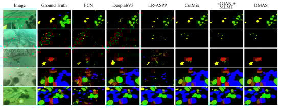
Figure 3. Visualization of comparative experimental results under 0.125 labeled ratio on UO datasets. The DMAS method demonstrates a significant advantage over the currently prevalent full-supervision semantic segmentation algorithms.

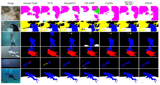
Figure 4. Visualization of comparative experimental results under 0.125 labeled ratio on SUIM datasets. DMAS excels in semi-supervised segmentation, outperforming full-supervision methods, despite minor edge delineation gaps.

4.5. Ablation Study

To further assess the rationality of the framework design choice in the DMAS method, we conducted ablation experiments on two underwater datasets. Initially, the baseline network consists of a fully supervised trained model within the DMAS method’s segmentation network, including Deeplabv3. Subsequently, this baseline network is enhanced with dynamic mutual learning. In contrast, the DMAS method not only incorporates the baseline network but also introduces model adversarial training and a dynamic mutual learning strategy. Under a labeling rate of 0.125, these experiments employed the same pre-trained dataset, trained on the training dataset, and subsequently evaluated on the test dataset. The quantitative analysis of the test sets for both datasets is illustrated in Figure 5. Training with the dynamic mutual learning method within the same experimental setup has significantly enhanced the model’s segmentation precision compared to solely using the baseline network. Concurrently, the inclusion of an adversarial training strategy has improved the algorithm’s overall performance. For discernible underwater targets, the mean Pixel Accuracy (mPA) exceeds 0.7, and for well-segmented instances, it can reach up to 0.8. This indicates that the dynamic mutual learning strategy can effectively utilize unlabeled data to extract associative information, thereby optimizing the segmentation model.

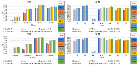
Figure 5. Quantitative comparison of ablation experiment results PA under 0.125 labeled ratio on SUIM dataset and UO dataset. Enhanced segmentation via dynamic mutual learning and adversarial strategy, achieving mPA exceeds $0.7$.

As illustrated by the visualization results in Figure 6 and Figure 7, models trained using the DMAS method can segment the majority of underwater target areas more proficiently. When faced with low-contrast and indistinct contour targets (as shown in the third row of Figure 6 and the second row of Figure 7), the models exhibit minimal classification errors and perform superior segmentation of small targets (as shown in the fourth row of Figure 6) and certain peripheral details. In the case of semantic segmentation of concealed targets (as shown in rows one and five of Figure 6), numerous errors still persist, yet there is a relative enhancement in classification accuracy compared to the other two methods.

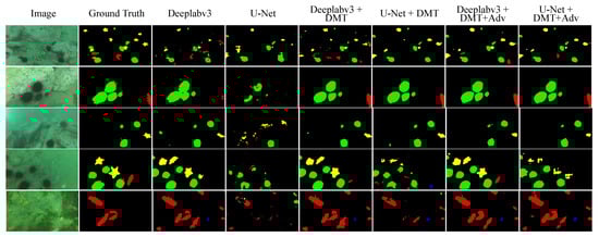
Figure 6. Visualization of ablation experimental results under 0.125 labeled ratio on UO datasets. Models trained using the DMAS method can segment the majority of underwater target areas more proficiently.

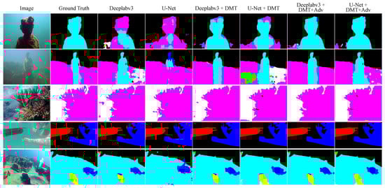
Figure 7. Visualization of ablation experimental results under 0.125 labeled ratio on SUIM datasets. Visualization of ablation experimental results under 0.125 labeled ratio on SUIM datasets. DMAS models excel in segmenting low-contrast underwater targets and peripheral details, reducing classification errors. However, concealed targets still present challenges.

To rigorously validate DMAS’s framework design rationality and quantitatively delineate the performance contribution of each core component, four controlled variants were designed under identical settings to isolate the effects of AP, DML, and $L_{DR}$—this extends the comparative scope of Figure 5. The four variants are a Baseline which is fully supervised DeepLabv3 without DMAS-specific components, Baseline+AP which integrates only adversarial pre-training to refine pseudo-label quality via a discriminator, Baseline+DML which incorporates only dynamic mutual learning to detect pseudo-label errors via inter-model divergence, and Full DMAS which is the complete framework integrating AP, DML, and dynamic reweighting loss $L_{DR}$ that adjusts pixel weights based on inter-model discrepancy to suppress high-error regions. Table 1 summarizes the quantitative results of these variants on DUT and SUIM datasets, reporting both mean Intersection over Union (mIoU) and mPA to comprehensively reflect segmentation performance. Adversarial Pre-training (AP) contributes a modest but critical 1.8% average gain, which comes from the discriminator’s ability to distinguish real label maps from model predictions, reducing noise in initial pseudo-labels and laying a reliable foundation for subsequent semi-supervised learning on DUT. Second, Dynamic Mutual Learning (DML) drives the most significant individual gain of 3.4% on average, as inter-model divergence effectively identifies pseudo-label errors that single-model self-training cannot detect, enabling more efficient utilization of unlabeled DUT data. Third, dynamic reweighting loss $L_{DR}$ adds an additional 1.4% average gain to Full DMAS, as its pixel-wise weight adjustment suppresses residual errors from DML on DUT, confirming its role as a “fine-grained error filter.” Notably, Full DMAS exhibits a synergistic effect on DUT: its 6.6% average gain equals the sum of individual component gains, which is attributed to AP’s high-quality pseudo-labels reducing DML’s error detection burden and $L_{DR}$ mitigating instability caused by inter-model interdependence, leading to super-additive performance improvement.

Table 1. Performance Contribution of DMAS Core Components on DUT and SUIM Datasets (Labeled Ratio = 0.125). Values in parentheses indicate absolute performance gain relative to the Baseline; Avg. Gain represents the average of mIoU and mPA gains across both datasets.

Model Variant	DUT mIoU	DUT mPA	SUIM mIoU	SUIM mPA	Avg. Gain vs. Baseline
Baseline	44.65	66.04	54.13	67.81	–
Baseline+AP	46.70 (+2.05)	67.50 (+1.46)	56.30 (+2.17)	69.40 (+1.59)	+1.8
Baseline+DML	48.20 (+3.55)	69.00 (+2.96)	58.00 (+3.87)	71.00 (+3.19)	+3.4
DMAS (Baseline + AP + DML + $L_{DR}$)	53.04 (+8.39)	72.17 (+6.13)	61.19 (+7.06)	72.48 (+4.67)	+6.6

To further elaborate on framework stability, evidence from controlled experiments on the DUT dataset is visualized in Figure 8. The figure includes training loss fluctuation trends, mPA and mIoU fluctuation distributions across different schemes, reflecting DMAS’s superior stability on DUT. DMAS stabilizes earlier and no longer improves with additional iterations, with its convergence speed outperforming the single-model baseline.

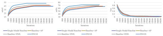
Figure 8. Training Stability Comparison Between DMAS and Single-Model Baseline on DUT Dataset (Labeled Ratio = 0.125). The figure includes training loss fluctuation trends, mPA and mIoU fluctuation distributions across different schemes, reflecting DMAS’s superior stability on DUT.

Computational complexity is another critical practical consideration for DMAS, as it directly affects deployment on resource-constrained underwater platforms. Table 2 quantifies this complexity against the single-model baseline. DMAS has 85.6 million trainable parameters, approximately twice the baseline’s 42.0 million—this increase stems from the dual segmentation networks and fully convolutional discriminator required for adversarial pre-training. DMAS requires 28 h of training, longer than the baseline’s 15 h, due to the additional computational load from its multi-component design. However, this overhead is justified by its performance gains: the synergistic AP+DML mechanism optimizes unlabeled data utilization, avoiding redundant iterations common in single-model pseudo-label training. For inference—critical for real-time underwater robot perception—DMAS achieves 18.3 FPS on 512 × 512 images, slightly lower than the baseline’s 19.5 FPS but still meeting the 15 FPS practical requirement for underwater perception systems. This balance between performance enhancement (6.6% average mIoU gain) and acceptable computational costs ensures DMAS’s viability for real-world underwater deployment, particularly given its superior performance in limited-label scenarios (8.39% mIoU gain on DUT, 7.06% on SUIM at 0.125 labeled ratio).

Table 2. Computational Complexity Comparison Between DMAS and Single-Model Baseline.

Metric	Trainable Parameters (M)	Training Time (h)	Inference Speed (FPS, 512 × 512)
Baseline	42.0	15	19.5
DMAS (AP + DML + $L_{DR}$)	85.6	28	18.3

4.6. Discussion

The increasing demand for advanced underwater detection and monitoring technologies has made underwater image semantic segmentation a prominent research area. Researchers are increasingly turning to convolutional neural networks (CNNs) and their variants. These models enhance the accuracy and robustness of segmentation. These models automatically learn hierarchical features, making them well-suited for addressing the complex patterns and textures characteristic of underwater scenes.

Despite these advancements, the field of underwater image semantic segmentation continues to face numerous challenges: (1) the lack of large annotated datasets limits the training and validation of deep learning algorithms. (2) Factors such as low visibility, poor contrast, and the presence of various underwater elements often contribute to significant annotation noise, thereby obscuring the segmentation results.

To tackle the challenges posed by limited noise annotations, many studies have proposed self-training methods, wherein models iteratively label and retrain on their predicted results. This method has been applied to underwater image segmentation. Especially when combined with confidence thresholds, this method can gradually enhance the model’s performance on noisy data. However, a notable limitation of self-training methodes is the lack of mechanisms to detect and correct errors during the training process. Furthermore, the choice of confidence threshold directly impacts the effective utilization of low-confidence pseudo-labels.

To address the issue of underwater image semantic segmentation with limited noisy annotations, we have developed more sophisticated solutions. By leveraging collaborative platforms and crowdsourcing techniques, we can aggregate multiple annotations, which helps reduce noise levels in the training dataset. Aggregated data validated through multiple sources can provide higher quality annotations. We enable dynamic mutual learning between two distinctly different models. Each model iteratively retrains on unannotated data, using pseudo-labels generated by the other model. This process allows the models to guide each other, enhancing their noise correction capabilities. Simultaneously, in selecting the confidence threshold for pseudo-label selection, we no longer rely on traditional confidence levels. Instead, inspired by generative adversarial concepts, we train a discriminator to focus on the performance of pseudo-labels, thereby making their selection more adaptive.

Our method significantly reduces noise levels in underwater image semantic segmentation, but there are still limitations that need to be addressed. Although dynamic mutual learning theoretically improves noise correction in models, its practical application can cause instability during training due to interdependencies among models, which affects convergence speed and overall performance. This is particularly evident in model selection, which consequently affects the efficacy of dynamic mutual learning. To tackle these challenges, we intend to integrate more advanced semantic segmentation network architectures, including multi-scale feature extraction and multi-task learning, to enhance the model’s ability to handle complex underwater environments. Furthermore, we plan to explore multimodal learning methods to improve the model’s robustness and generalization by integrating diverse sensor data, including vision and sonar.

5. Conclusions

This paper introduces a novel semi-supervised method for underwater image semantic segmentation, named Dynamic Mutual Adversarial Segmentation (DMAS). The method employs a two-stage framework: adversarial pre-training and dynamic mutual learning. In the adversarial pre-training stage, the segmentation model is initially trained using labeled data to generate pseudo-labels. Concurrently, a convolutional discriminator is trained on both the segmentation maps derived from labeled and unlabeled data. This dual training process enables the network to differentiate between actual and predicted labels by producing a confidence map, which aids in qualitatively assessing the segmentation accuracy. During the dynamic mutual learning stage, multiple models with different prior knowledge are trained. By analyzing the divergence between these models, errors in the pseudo-labels can be detected. The training process incorporates a dynamically reweighted loss function, which adjusts weights based on the differences between the models. This method reduces the impact of discrepancies that suggest potential errors, thereby improving the precision of the training process. Experimental results on the DUT and SUIM datasets indicate that DMAS significantly enhances semantic segmentation performance, even with a limited amount of labeled data. To promote the reproducibility and application of this work, the code and pre-trained models of the DMAS framework will be released on a public https://github.com/chenhan216003/DMAS (accessed on 25 November 2025)repository after the paper is formally accepted.

References

- McNelly, B.P. Advances in Autonomous Underwater Vehicle Technologies for Enhanced Harbor Protection. Ph.D. Thesis, Johns Hopkins University, Baltimore, MD, USA, 2023. [Google Scholar]
- Li, Z.; Liang, S.; Guo, M.; Zhang, H.; Wang, H.; Li, Z.; Li, H. Adrc-based underwater navigation control and parameter tuning of an amphibious multirotor vehicle. IEEE J. Ocean. Eng. 2024, 49, 775–792. [Google Scholar] [CrossRef]
- Yang, X.; Song, Z.; King, I.; Xu, Z. A survey on deep semi-supervised learning. IEEE Trans. Knowl. Data Eng. 2022, 35, 8934–8954. [Google Scholar] [CrossRef]
- Zeng, H.; Liu, Z.; Cai, H. Research on the application of deep learning in computer network information security. J. Phys. Conf. Ser. 2020, 1650, 032117. [Google Scholar] [CrossRef]
- Zhang, M.; Zhou, Y.; Zhao, J.; Man, Y.; Liu, B.; Yao, R. A survey of semi-and weakly supervised semantic segmentation of images. Artif. Rev. 2020, 53, 4259–4288. [Google Scholar] [CrossRef]
- Li, Q.; Wu, X.-M.; Liu, H.; Zhang, X.; Guan, Z. Label efficient semi-supervised learning via graph filtering. In Proceedings of the IEEE/CVF Conference on Computer Vision and Pattern Recognition, Long Beach, CA, USA, 15–20 June 2019; pp. 9582–9591. [Google Scholar]
- Wei, Y.; Xiao, H.; Shi, H.; Jie, Z.; Feng, J.; Huang, T.S. Revisiting dilated convolution: A simple approach for weakly-and semi-supervised semantic segmentation. In Proceedings of the IEEE Conference on Computer Vision and Pattern Recognition, Salt Lake City, UT, USA, 18–23 June 2018; pp. 7268–7277. [Google Scholar]
- Ouali, Y.; Hudelot, C.; Tami, M. Semi-supervised semantic segmentation with cross-consistency training. In Proceedings of the IEEE/CVF Conference on Computer Vision and Pattern Recognition, Seattle, WA, USA, 14–19 June 2020; pp. 12674–12684. [Google Scholar]
- Lee, D.-H. Pseudo-label: The simple and efficient semi-supervised learning method for deep neural networks. Work. Chall. Represent. Learn. ICML 2013, 3, 896. [Google Scholar]
- Li, R.; Li, S.; He, C.; Zhang, Y.; Jia, X.; Zhang, L. Class-balanced pixel-level self-labeling for domain adaptive semantic segmentation. In Proceedings of the IEEE/CVF Conference on Computer Vision and Pattern Recognition, New Orleans, LA, USA, 18–24 June 2022; pp. 11593–11603. [Google Scholar]
- Triguero, I.; García, S.; Herrera, F. Self-labeled techniques for semi-supervised learning: Taxonomy, software and empirical study. Knowl. Inf. Syst. 2015, 42, 245–284. [Google Scholar] [CrossRef]
- Chapelle, O.; Scholkopf, B.; Zien, A. Semi-Supervised Learning; MIT Press: Cambridge, MA, USA, 2006. [Google Scholar]
- Yang, L.; Zhuo, W.; Qi, L.; Shi, Y.; Gao, Y. St++: Make self-training work better for semi-supervised semantic segmentation. In Proceedings of the IEEE/CVF Conference on Computer Vision and Pattern Recognition, New Orleans, LA, USA, 18–24 June 2022; pp. 4268–4277. [Google Scholar]
- Teh, E.W.; DeVries, T.; Duke, B.; Jiang, R.; Aarabi, P.; Taylor, G.W. The gist and rist of iterative self-training for semi-supervised segmentation. In Proceedings of the 2022 19th Conference on Robots and Vision (CRV), Toronto, ON, Canada, 31 May–2 June 2022; IEEE: New York, NY, USA, 2022; pp. 58–66. [Google Scholar]
- Li, H.; Zheng, H. A residual correction approach for semi-supervised semantic segmentation. In Proceedings of the Pattern Recognition and Computer Vision: 4th Chinese Conference, PRCV 2021, Beijing, China, 29 October–1 November 2021; Proceedings, Part IV 4. Springer: Berlin/Heidelberg, Germany, 2021; pp. 90–102. [Google Scholar]
- Yuan, J.; Liu, Y.; Shen, C.; Wang, Z.; Li, H. A simple baseline for semi-supervised semantic segmentation with strong data augmentation. In Proceedings of the IEEE/CVF International Conference on Computer Vision, Montreal, BC, Canada, 11–17 October 2021; pp. 8229–8238. [Google Scholar]
- Zhang, Y.; Xiang, T.; Hospedales, T.M.; Lu, H. Deep mutual learning. In Proceedings of the IEEE Conference on Computer Vision and Pattern Recognition, Salt Lake City, UT, USA, 18–22 June 2018; pp. 4320–4328. [Google Scholar]
- Feng, Z.; Zhou, Q.; Gu, Q.; Tan, X.; Cheng, G.; Lu, X.; Shi, J.; Ma, L. Dmt: Dynamic mutual training for semi-supervised learning. Pattern Recognit. 2022, 130, 108777. [Google Scholar] [CrossRef]
- Zhou, Y.; Jiao, R.; Wang, D.; Mu, J.; Li, J. Catastrophic forgetting problem in semi-supervised semantic segmentation. IEEE Access 2022, 10, 48855–48864. [Google Scholar] [CrossRef]
- Creswell, A.; White, T.; Dumoulin, V.; Arulkumaran, K.; Sengupta, B.; Bharath, A.A. Generative adversarial networks: An overview. IEEE Signal Process. Mag. 2018, 35, 53–65. [Google Scholar] [CrossRef]
- Gui, J.; Sun, Z.; Wen, Y.; Tao, D.; Ye, J. A review on generative adversarial networks: Algorithms, theory, and applications. IEEE Trans. Knowl. Data Eng. 2021, 35, 3313–3332. [Google Scholar] [CrossRef]
- Wang, Z.; She, Q.; Ward, T.E. Generative adversarial networks in computer vision: A survey and taxonomy. Acm Comput. Surv. (CSUR) 2021, 54, 1–38. [Google Scholar] [CrossRef]
- Souly, N.; Spampinato, C.; Shah, M. Semi supervised semantic segmentation using generative adversarial network. In Proceedings of the IEEE International Conference on Computer Vision, Venice, Italy, 22–29 October 2017; pp. 5688–5696. [Google Scholar]
- Li, D.; Yang, J.; Kreis, K.; Torralba, A.; Fidler, S. Semantic segmentation with generative models: Semi-supervised learning and strong out-of-domain generalization. In Proceedings of the IEEE/CVF Conference on Computer Vision and Pattern Recognition, Nashville, TN, USA, 19–25 June 2021; pp. 8300–8311. [Google Scholar]
- Jin, G.; Liu, C.; Chen, X. Adversarial network integrating dual attention and sparse representation for semi-supervised semantic segmentation. Inf. Process. Manag. 2021, 58, 102680. [Google Scholar] [CrossRef]
- Xu, D.; Wang, Z. Semi-supervised semantic segmentation using an improved generative adversarial network. J. Intell. Fuzzy Syst. 2021, 40, 9709–9719. [Google Scholar] [CrossRef]
- Mendel, R.; Souza, L.A.D.; Rauber, D.; Papa, J.P.; Palm, C. Semi-supervised segmentation based on error-correcting supervision. In Proceedings of the Computer Vision–ECCV 2020: 16th European Conference, Glasgow, UK, 23–28 August 2020; Proceedings, Part XXIX 16. Springer: Berlin/Heidelberg, Germany, 2020; pp. 141–157. [Google Scholar]
- Ke, Z.; Qiu, D.; Li, K.; Yan, Q.; Lau, R.W. Guided collaborative training for pixel-wise semi-supervised learning. In Proceedings of the Computer Vision–ECCV 2020: 16th European Conference, Glasgow, UK, 23–28 August 2020; Proceedings, Part XIII 16. Springer: Berlin/Heidelberg, Germany, 2020; pp. 429–445. [Google Scholar]
- Hung, W.-C.; Tsai, Y.-H.; Liou, Y.-T.; Lin, Y.-Y.; Yang, M.-H. Adversarial learning for semi-supervised semantic segmentation. arXiv 2018, arXiv:1802.07934. [Google Scholar] [CrossRef]
- Zhang, J.; Li, Z.; Zhang, C.; Ma, H. Stable self-attention adversarial learning for semi-supervised semantic image segmentation. J. Vis. Commun. Image Represent. 2021, 78, 103170. [Google Scholar] [CrossRef]
- Luc, P.; Couprie, C.; Chintala, S.; Verbeek, J. Semantic segmentation using adversarial networks. arXiv 2016, arXiv:1611.08408. [Google Scholar] [CrossRef]
- Yurtkulu, S.C.; Şahin, Y.H.; Unal, G. Semantic segmentation with extended deeplabv3 architecture. In Proceedings of the 2019 27th Signal Processing and Communications Applications Conference (SIU), Sivas, Turkey, 24–26 April 2019; IEEE: New York, NY, USA, 2019; pp. 1–4. [Google Scholar]
- Long, J.; Shelhamer, E.; Darrell, T. Fully convolutional networks for semantic segmentation. In Proceedings of the IEEE Conference on Computer Vision and Pattern Recognition, Boston, MA, USA, 7–12 June 2015; pp. 3431–3440. [Google Scholar]
- Howard, A.; Sandler, M.; Chu, G.; Chen, L.-C.; Chen, B.; Tan, M.; Wang, W.; Zhu, Y.; Pang, R.; Vasudevan, V.; et al. Searching for mobilenetv3. In Proceedings of the IEEE/CVF International Conference on Computer Vision, Seoul, Republic of Korea, 27 October–2 November 2019; pp. 1314–1324. [Google Scholar]
- French, G.; Laine, S.; Aila, T.; Mackiewicz, M.; Finlayson, G. Semi-supervised semantic segmentation needs strong, varied perturbations. arXiv 2019, arXiv:1906.01916. [Google Scholar]
- Mittal, S.; Tatarchenko, M.; Brox, T. Semi-supervised semantic segmentation with high-and low-level consistency. IEEE Trans. Pattern Anal. Mach. Intell. 2019, 43, 1369–1379. [Google Scholar] [CrossRef] [PubMed]
Disclaimer/Publisher’s Note: The statements, opinions and data contained in all publications are solely those of the individual author(s) and contributor(s) and not of MDPI and/or the editor(s). MDPI and/or the editor(s) disclaim responsibility for any injury to people or property resulting from any ideas, methods, instructions or products referred to in the content. |
© 2025 by the authors. Licensee MDPI, Basel, Switzerland. This article is an open access article distributed under the terms and conditions of the Creative Commons Attribution (CC BY) license (https://creativecommons.org/licenses/by/4.0/).