Collision Avoidance Strategies for Unmanned Surface Vehicles Based on Improved RRT Algorithm

Abstract

In order to solve the problem of obstacle avoidance for unmanned surface vehicles (USV), based on the classic RRT algorithm and Velocity Obstacle principle, an improved RRT algorithm is proposed. For the situation of the extension direction of the parent node inside the collision cone in the EXTEND operation, ‘obstacle repellent vector’ and ’collision risk index’ are presented, making the extension direction of the search tree have the tendency to move away from obstacle. Meanwhile for the problem of the real time performance of the algorithm and path oscillation, ‘target attraction vector’ and waypoint corner constraint are introduced to accelerate the convergence of the algorithm and improve the quality of path point. Path planning experiment results show that the improved algorithm has better real-time character. Path tracking experiment results based on 3-DOF ship nonlinear dynamic model reveal that the collision-free paths generated by improved RRT algorithm are smoother and the navigation time is shorter, which are of great significance for practical engineering application.

1. Introduction

With the continuous development of artificial intelligence, unmanned systems have been continuously popularized and applied, becoming an indispensable part of people’s daily life and receiving increasing attention from the governments of many countries. As a typical type of maritime unmanned system, unmanned surface vehicles (USV) can be used in anti-submarine, reconnaissance, and cluster operations in military applications, and can be used in marine exploration, water quality monitoring, and port patrol in scientific research and livelihood projects. Therefore, USVs have great significance in academic research and engineering applications. To fully implement the autonomy of USVs, it is essential to make the ship capable of intelligent navigation in the marine environment, of which the most essential capability is avoiding collisions with obstacles based on the planning of high-quality routes through the detection and collection of environmental information by the sensing system. It is also necessary to differentiate the task from collision avoidance of general robot systems. The fact that the research object of unmanned collision avoidance is the ship poses a challenge for the task. Publicized data shows that about half of the casualties at sea from 2011 to 2015 were from navigation tasks, and more than 80% of crashes were caused by the wrong decision of seafarers [1]. The data reflect the difficulty of planning and manipulating ships to avoid obstacles. The author believes that the root causes of such difficulties are the under-actuated motion system, strong nonlinear dynamic characteristics, and huge inertia of ships. These characteristics impose higher requirements on the quality of planning of the collision avoidance path points, the real-time nature of the collision avoidance algorithm, and the navigation status of the planned path points in actual ship tracking and tracing.

The existing advanced technologies on collision avoidance planning for USV can be roughly divided into three categories. The first is based on the most widely studied and applied method of the artificial potential field [2,3,4]. The method of the artificial potential field has prominent advantages. It is simple and practical, and it is conducive to underlying control. However, the existing achievements rarely start from the requirements of the quality of the waypoint planning and the real-time calculation requirements brought by the special situation of ship avoidance. The second is based on the principle of Velocity Obstacle (VO) [5,6]. The basic idea of this method is to mathematically solve all the velocity sets that may cause the target to collide with the obstacle and calculate the feasible heading of the ship under the condition that the ship and the obstacle maintain the current state of motion. However, the ship usually has a large inertia, the mathematically calculated heading angle usually makes it difficult for USV to adjust in time. The third is based on the application of other intelligent algorithms, such as multi-objective optimization interval method [7], heuristic A* algorithm [8], and DPSS algorithm [9]. However, for the strong dynamic nonlinear system of unmanned ships, the simple connection and fitting between the planned path points and the final route shown by the actual ship in the marine environment are usually quite different.

In order to solve the above problems to some extent, in this paper, based on the classic RRT algorithm and VO principle, an improved RRT algorithm (hereinafter referred to as V-RRT algorithm) is proposed, the innovation of the proposed V-RRT algorithm and related research lies in the following. (1) ‘Obstacle repellent vector’ design based on the VO principle. During each iteration, the method can automatically identify whether the parent node’s extension direction is located in the cone collision area and dynamically adjust the amplitude of the obstacle repulsion vector according to the collision avoidance risk coefficient, making the collision avoidance path more reasonable and efficient. (2) ‘Target attraction vector’ design, the method excites the target point attraction vector when the search tree extension direction deviates greatly from the target point, so as to solve the problem and improve the real-time performance and convergence speed of the algorithm. (3) The method introduces the corner constraint of adjacent path points to reduce path oscillation. More importantly, in order to evaluate and test the quality of the V-RRT algorithm proposed in this paper, based on the 3-DOF nonlinear dynamic model of the ship, simulation experiments and analysis of the performance characteristics and responses reflected during the actual tracking were carried out.

2. Related Work

The Rapidly Exploring Random Tree (RRT) algorithm, first introduced by Lavalle [10], has gained widespread adoption in recent years as a path planning solution for robots and UAVs [11,12,13]. Its primary advantages include ideal real-time performance, as it incrementally expands the search tree toward an unknown state space via random sampling, avoiding space modeling and minimizing computational complexity even with increasing obstacles. Studies show that, compared to algorithms like A*, MILP, and PRM, RRT achieves faster convergence and greater planning efficiency [14,15,16,17]. Additionally, the EXTEND step in the RRT algorithm offers considerable optimization flexibility, making it suitable for incorporating dynamic constraints, especially in unmanned ship applications. Moreover, RRT is effective in complex motion planning scenarios involving multi-degree-of-freedom mobile robots or multi-dimensional pose spaces. However, the RRT algorithm has certain drawbacks, including instability, lack of orientation, and path oscillation. To address these issues, various improvements have been proposed. For instance, the DT-RRT algorithm by Moon et al. [18] tackles the lack of orientation by using a dual tree structure—one for workspace and one for state-space—enabling high-speed navigation in two-wheel differential robots. G.-Y. Yin and S.-L. Zhou [19] improved RRT path planning in UAV applications by introducing path length constraints and optimizing root node selection. Additionally, Heo and Chung [20] combined the A* and RRT algorithms for Autonomous Underwater Vehicle (AUV) motion planning, where RRT manages local path planning under motion constraints, while A* finds the shortest path to avoid obstacles. Despite these improvements, research on optimizing RRT for unmanned surface vehicle (USV) applications remains limited, with most approaches focusing on virtual obstacles to satisfy COLREG regulations [21] or improving growth/exploration points [22]. There is a clear gap in optimizing the EXTEND step and validating tracking points in USV-related RRT implementations.

3. Preliminaries

3.1. Ship Kinematics and Dynamics

In this letter, we discuss the 3 DOF ship model using nonlinear differential equations. Neglecting the heave, roll, and pitch, we can describe the ship kinematic mathematical model as [23]

$$\dot{\eta }=R(\psi )v$$

(1)

With $\eta ={[x,y,\psi ]}^T$, $v={[u,v,r]}^T$, and the rotation matrix $R(\psi )$:

$$R(\psi )=\left[\begin{array}{ccc}\cos \psi & -\sin \psi & 0\\ \sin \psi & \cos \psi & 0\\ 0& 0& 1\end{array}\right]$$

(2)

The ship dynamics mathematical model can be denoted as

$$M_{RB}\dot{v}+C_{RB}(v)v+M_A{\dot{v}}_r+C_A(v_r)v_r+D_L(v_r)v_r+D_N(v_r)v_r+g(\eta )+g_0=\tau +{\tau }_{wind}+{\tau }_{wave}. \tau =B_u{u}_p$$

(3)

With

$$\begin{array}{c}{M}_{RB}=\left[\begin{array}{ccc}m& 0& 0\\ 0& m& m{x}_g\\ 0& m{x}_g& I_z\end{array}\right]C_{RB}(v)=\left[\begin{array}{ccc}0& 0& -m(x_{g}r+v)\\ 0& 0& mu\\ m(x_{g}r+v)& -mu& 0\end{array}\right]\\ M_A=\left[\begin{array}{ccc}-X_{\dot{u}}& 0& 0\\ 0& -Y_{\dot{v}}& -Y_{\dot{r}}\\ 0& -Y_{\dot{r}}& -N_{\dot{r}}\end{array}\right]C_A(v_r)=\left[\begin{array}{ccc}0& 0& Y_{\dot{v}}{v}_r+Y_{\dot{r}}r\\ 0& 0& -X_{\dot{u}}{u}_r\\ -Y_{\dot{v}}{v}_r-Y_{\dot{r}}r& X_{\dot{u}}{u}_r& 0\end{array}\right]\\ D(v_r)=D_L(v_r)v_r+D_N(v_r)v_r=\left[\begin{array}{ccc}-X_{\left|u\right|u}\left|u_r\right|& 0& 0\\ 0& -Y_{\left|v\right|v}\left|v_r\right|-Y_{\left|r\right|v}\left|r\right|& -Y_{\left|v\right|r}\left|v_r\right|-Y_{\left|r\right|r}\left|r\right|\\ 0& -N_{\left|v\right|v}\left|v_r\right|-N_{\left|r\right|v}\left|r\right|& -N_{\left|v\right|r}\left|v_r\right|-N_{\left|r\right|r}\left|r\right|\end{array}\right]\\ B_u=\left[\begin{array}{cc}1-t_p& 0\\ 0& Y_{\delta }\\ 0& N_{\delta }\end{array}\right] u_p=\left[\begin{array}{c}{T}_{pc}\\ {\delta }_c\end{array}\right]\end{array}$$

(4)

where $M_{RB}$ is the rigid body inertia matrix, $C_{RB}(v)$ is the rigid-body Coriolis and centripetal matrix, $M_A$ is the added mass inertial matrix, $C_A$ is the added mass inertial Coriolis and centripetal matrix, $D(v_r)$ is the damping matrix, $B_u$ is the ship actuator configuration matrix, and $u_p$ is the vector of control inputs including propeller thrust and rudder angle. From the form of the elements contained in each matrix, $M_{RB}$ can be calculated by the basic information of the ship, such as mass, center of gravity vertical coordinate and moment of inertia. $M_A$, $C_A$, $C_{RB}(v)$ can be calculated by real-time ship motion state and hydrodynamic coefficient. In this letter, both the linear potential damping $D_L(v_r)$ and nonlinear quadratic terms $D_n(v_r)$ are considered.

3.2. RRT Basics

The classic RRT Algorithm 1 flow is as follows [10]:

Algorithm 1: RRT

BUILD_RRT

1 $T$.init($X_{init}$);

2   for k = 1 to $K$ do

3  $X_{rand}$←RANDOM_STATE();

4  EXTEND($T$, $X_{rand}$)

5   Return $T$

EXTEND($T,x$)

1 $x_{near}\leftarrow NEAREST\_NEIGHBOR(x,T)$;

2 $u\leftarrow \mathrm{SAMPLE}\_CONTROL\_INPUT$

3 $x_{\mathit{new}}\leftarrow PROPAGATE(x_{near},u)$

4 if NEW_STATEMENT($x,x_{near},x_{new}$)

5  $T.$add_vertex($x_{new}$);

6  $T.$add_edge($x_{near},x_{new}$);

7  if $x_{new}=x$ then

8   Return Reached;

9  else

10   Return Advanced;

11 Return Trapped;

The key point of classic RRT algorithm is sampling nodes in the state space to extend the search tree toward the unknown space. We briefly explain the general implementation steps of the RRT: Firstly, we define the configuration space as $C$

$$C=C_{free}\cup C_{obs}(C_{free}\cap C_{obs}=\varnothing )$$

where $C_{free}$ is the free space, $C_{obs}$ is the obstacle space. Meanwhile we define the initial position and target position as $X_{init}$ and $X_{goal}$, respectively. Then choosing the $X_{init}$ as root node of the random tree and $X_{rand}$ is randomly sampled from the configuration space. Next, selecting a nearest node to $X_{rand}$ from all the node in the random tree named $X_{near}$, a distance of ${\epsilon }_0$ is extended from the direction of $X_{near}$ to obtain a new node named $X_{new}$. During the extension process, if $X_{new}\notin C_{obs}$, $X_{new}$ will be accepted and will be added as a node of the tree; if $X_{new}\in C_{obs}$, $X_{new}$ will be discarded and $X_{rand}$ will be generated again. Through such continuous extension and expansion, when the distance from the node of the random tree closest to the $X_{goal}$ to $X_{goal}$ is less than or equal to ${\epsilon }_0$, the construction process of the random tree can be regarded as successful. The schematic diagram of the construction process is shown in Figure 1.

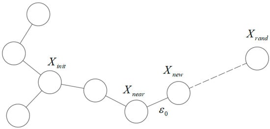
Figure 1. The construction process of classic RRT algorithm.

3.3. Velocity Obstacle Principle

When we consider the situation of the USV collision avoidance, the most basic thing is the environment modeling. USV can obtain environmental information through radar, AIS, and other equipment when performing navigation tasks. Through the environmental information, the bearing, shape, and other information of the obstacles that hinder the safe navigation can be extracted and stored; then, we can build USV–Obstacle environmental model to determine collision area as shown in Figure 2. At time t, the USV A emits rays $l_a(\rho ,{\theta }_a)$ and $l_b(\rho ,{\theta }_b)$ to the tangential direction of obstacle B. The relative velocity of USV and obstacle is $v_R$, the angle between $v_R$ and the x-axis is ${\theta }_R$. The obstacle B center coordinates are (x, y). The following mathematical relationships exist:

$$\begin{array}{l}x=x_0+S_{ab}\cos {\theta }_0\\ y=y_0+S_{ab}\sin {\theta }_0\end{array}$$

(5)

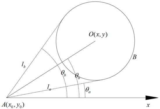
Figure 2. USV–Obstacle environmental model based on the VO principle.

With ${\theta }_0={\displaystyle \frac{1}{2}}({\theta }_a+{\theta }_b)$, $S_{ab}={\displaystyle \frac{\rho }{\cos (({\theta }_b-{\theta }_a)/2)}}$.

According to the principle of Velocity Obstacle principle proposed by Fiorini [24], assuming that all angles have a range of $[0,2\pi ]$, clockwise rotation is positive, the condition that the USV collides with the obstacle is ${\theta }_a<{\theta }_R<{\theta }_b$, and this region is defined as cone collision zone.

The principle of Velocity Obstacle provides a simple and efficient basis for how to change and control the heading during the collision avoidance process of the USV. It also improves the theoretical basis for the application and improvement of the classic RRT algorithm in the collision avoidance of USV.

4. Method

Although the classic RRT algorithm has characteristics such as fast convergence, for it to be applied to USV for collision avoidance, there are still the following problems. (1) The extension direction of the search tree in the extension step is too random, and it may extend towards the direction of the obstacle, so that the direction of the unmanned ship will hit the obstacle in some sections. (2) The direction of search tree extension shifts the target point in some sections, increasing the unnecessary consumption of the algorithm, reducing the quality and real-time performance of the path. (3) Path oscillation; excessive turning angles between some path points do not meet the requirement of path cornering constraints caused by the ship’s dynamic constraints and rudder angle restrictions.

In this paper, regarding the issues above, the V-RRT algorithm is proposed. The symbol stipulates that the search tree $T$ is initialized with the current position $X_{init}$ of the USV. The search tree during a certain iteration generates a random point $P_r$($X_r,Y_r$), and the node in the tree that is closest to the random point is $P_p$($X_p,Y_p$). Section 3.2 shows that $P_p$ will be used as the parent node in this iteration to extend the exploration step-size $S$ to $P_r$. The resulting child node is $P_n$$(X_n,Y_n)$. The coordinate of the obstacle is $P_o$ ($X_o,Y_o$), and the obstacle’s expansion radius is $R$.

4.1. ‘Object Repellent Vector’ Design

When the classic RRT algorithm generates random points, if it guides the search tree toward the obstacle, expressing in the USV collision avoidance model, it is the random point that guides the USV’s course to adjust to the cone collision area defined in VO principle. At best, it increases the probability that subsequent nodes will extend the standard stride and fall into the obstacle area, increasing the unnecessary consumption of the algorithm; at worst, it prevents the algorithm from converging and makes the algorithm unable to plan an effective collision avoidance path. In view of the above issue, in this paper, an EXTEND step of the obstacle exclusion vector V-RRT algorithm based on the VO principle is proposed. The method can automatically identify whether the extension direction of the parent node is located in the cone collision area during each iteration and dynamically adjusts the strength of the obstacle repulsion vector according to the collision avoidance risk coefficient, thus making the collision avoidance path more reasonable and efficient.

Based on the EXTEND step of the RRT algorithm, the coordinate of extended node $P_n$($X_n,Y_n$) is calculated as in Formula (6):

$$\begin{array}{c}{X}_n=X_p+S\times \cos (\arctan ({\displaystyle \frac{Y_r-Y_p}{X_r-X_p}}))\\ Y_n=Y_p+S\times \sin (\arctan ({\displaystyle \frac{Y_r-Y_p}{X_r-X_p}}))\end{array}$$

(6)

With vector representation, Formula (6) is equivalent to Formula (7):

$$\overrightarrow{P_p{P}_n}=S\times {\displaystyle \frac{\overrightarrow{P_p{P}_r}}{\left|\overrightarrow{P_p{P}_r}\right|}}$$

(7)

If this extension leads the USV’s heading to the cone collision area, then Formula (8) is geometrically satisfied:

$${\alpha }_1<{\theta }_1$$

(8)

In Formula (8), ${\alpha }_1$, ${\theta }_1$ are from Formulas (9) and (10):

$${\alpha }_1=\arccos ({\displaystyle \frac{\overrightarrow{P_p{P}_n}•\overrightarrow{P_p{P}_o}}{\left|\overrightarrow{P_p{P}_n}\right|\times \left|\overrightarrow{P_p{P}_o}\right|}})$$

(9)

$${\theta }_1=\arcsin ({\displaystyle \frac{R}{\left|\overrightarrow{P_p{P}_o}\right|}})$$

(10)

At this point, the ‘obstacle repellent vector’ $\overrightarrow{R}$ and the collision avoidance risk coefficient $\omega$ in the V-RRT algorithm in this paper are triggered. $\overrightarrow{R}$ is defined in Formula (11) and $\omega$ is defined in Formula (12). Under the effect of $\overrightarrow{R}$ and $\omega$, the extended child node $P_n$ and its coordinates no longer satisfy Formula (6), and $P_n^{\prime }$ is given by Formula (13):

$$\overrightarrow{R}=\omega \times S\times {\displaystyle \frac{\overrightarrow{P_o{P}_p}}{\left|\overrightarrow{P_o{P}_p}\right|}}$$

(11)

$$\omega ={(\tanh ({\displaystyle \frac{2\times \left|\overrightarrow{P_p{P}_o}\right|}{L_s}}))}^{-1}$$

(12)

$$\begin{array}{l}\overrightarrow{V}=S\times {\displaystyle \frac{\overrightarrow{P_p{P}_r}}{\left|\overrightarrow{P_p{P}_r}\right|}}+\overrightarrow{R}\\ \overrightarrow{P_p{P}_n^{\prime }}=S\times {\displaystyle \frac{\overrightarrow{V}}{\left|\overrightarrow{V}\right|}}\end{array}$$

(13)

Formula (13) shows that when the extension direction of the parent node $P_p$ is within the cone collision area, USV has a dangerous heading. The ‘obstacle repellent vector’ $\overrightarrow{R}$ dynamically adjusted the original extension of search tree in the direction of the line from $P_o$ to $P_p$ according to the collision avoidance risk coefficient $\omega$, increasing the tendency of the extension of the search tree to stay away from obstacles. This process can be geometrically expressed as in Figure 3.

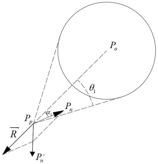
Figure 3. The action of $\overrightarrow{R}$ and $\omega$.

In Formula (12), $L_s$ is the critical distance for safe collision avoidance, and the core function is the hyperbolic tangent function $y=\tanh (x)$. The function’s graph is shown in Figure 4:

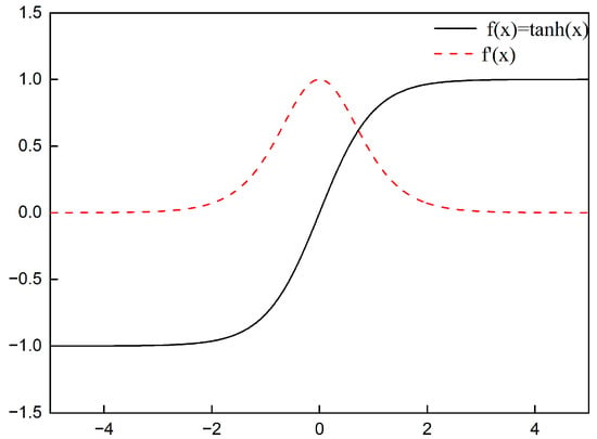
Figure 4. Graph of hyperbolic tangent function.

Figure 4 shows that, the part of the function $y=\tanh (x)$ located on the positive x-axis has the following characteristics: (1) when inputting $x\in (0,2)$, $y\in \left[0,1\right]$ and the value change drastically; (2) when inputting $x\in \left(2,+\infty \right)$, output y starts to be insensitive to changes in x; when $\left|\overrightarrow{P_o{P}_p}\right|>L_s$, as $\left|\overrightarrow{P_o{P}_p}\right|$ increases, according to Characteristic 2, the value of $\omega$ remains near 1 at this time; in terms of obstacle avoidance on USV, it is reflected in the fact that when the parent node meets a certain safety distance from the center of the obstacle, the obstacle exclusion vector has no obvious effect; when $\left|\overrightarrow{P_o{P}_p}\right|<L_s$, as $\left|\overrightarrow{P_o{P}_p}\right|$ decreases, according to Characteristic 1, the value of $\omega$ increases drastically; in terms of obstacle avoidance on USV, it is reflected in the fact that the closer the parent node is to the center of the obstacle, the more obvious the obstacle repulsion vector is, and the direction of extension, that is, the direction of the USV will be farther away from the obstacle.

4.2. ‘Targrt Attraction Vector’ Design

Similarly to the ‘obstacle repellent vector’ in Section 3.1, the ‘target attraction vector’ is stimulated under specific conditions, so that the search tree extension direction plays a corrective role when the deviation from the target point is large.

In an iteration process, suppose a search tree obtains $P_n$ according to Formula (6) of Section 3.1, if ${\alpha }_1$ is obtained from Formulas (9) and (10), ${\theta }_1$ satisfy Formula (14):

$${\alpha }_1>{\theta }_1$$

(14)

At this point, the ‘target attraction vector’ $\overrightarrow{A}$ in V-RRT algorithm in this paper will be triggered. $\overrightarrow{A}$ is defined by Formula (15). With the effect of $\overrightarrow{A}$, the extended child node $P_n$ and its coordinates no longer satisfy Formula (6), and $P_n^{\prime }$ is given by Formula (16):

$$\overrightarrow{A}=S\times {\displaystyle \frac{\overrightarrow{P_p{P}_g}}{\left|\overrightarrow{P_p{P}_g}\right|}}$$

(15)

$$\begin{array}{l}\overrightarrow{U}=S\times {\displaystyle \frac{\overrightarrow{P_p{P}_r}}{\left|\overrightarrow{P_p{P}_r}\right|}}+\overrightarrow{A}\\ \overrightarrow{P_p{P_n}^{″}}=S\times {\displaystyle \frac{\overrightarrow{U}}{\left|\overrightarrow{U}\right|}}\end{array}$$

(16)

In Formula (15), $P_g$ is the coordinate of the target point. Formula (16) shows that when the direction of the parent node’s extension is outside the cone collision area defined in VO principle, the USV’s heading is safe. The ‘target attraction vector’ $\overrightarrow{A}$ from $P_p$ to $P_g$ on the basis of the original extension will be added to make the search tree grow towards the target point. This process can be geometrically expressed as in Figure 5.

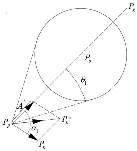
Figure 5. The action of $\overrightarrow{A}$.

It should be emphasized that while the vectors $\overrightarrow{R}$ and $\overrightarrow{A}$ enhance the collision avoidance and convergence behaviors, they do not guarantee the avoidance of local minima. As the RRT algorithm itself is not optimal and relies on randomness, the resulting paths may still encounter local minima under certain conditions.

4.3. Design of Method for Waypoint Corner Constraint

The classic RRT algorithm is based on random search, and the search tree extends towards random points. This extension method is highly random, and the quality of the path depends on the points randomly generated in each search. The planned path often has many twists and turns, and the corner of the path is often large. It is even often the case that the corner is larger than the maximum turning angle of the USV, so the path often has poor quality. Due to maneuverability constraints, it is difficult for ships to track such a path, and tracking such a path would unnecessarily consume mission time and increase navigation costs.

In this paper, for the above issues, a corner constraint is applied to each extended new node to limit the randomness of the classic RRT algorithm and reduce path oscillation. After calculating the extended child node coordinate $P_n$($X_n,Y_n$) according to Formula (6), the rotation constraint inspection is performed on $P_n$. The specific method is as follows. Extend parent node $p_p$ of child node $P_n$, and trace back to parent node $P_f$ of $P_p$, establish vector $\overrightarrow{p_f{p}_p}$ and calculate the angle β between vector $\overrightarrow{p_f{p}_p}$ and vector $\overrightarrow{p_p{p}_n}$, as shown in Formula (17). When it is determined that $\beta >\theta$ ($\theta$ is the maximum turning angle of the USV), that is, $P_n$ does not satisfy the corner constraint, abandon node $P_n$, and regenerate random points for the next search. When $\beta \le \theta$, the extension is successful.

$$\beta =\arccos ({\displaystyle \frac{\overrightarrow{P_p{P}_n}•\overrightarrow{P_f{P}_p}}{\left|\overrightarrow{P_p{P}_n}\right|\times \left|\overrightarrow{P_f{P}_p}\right|}})$$

(17)

The V-RRT Algorithm 2 flow can be written as

Algorithm 2: V-RRT

BUILD_V-RRT

1 $T$.init($X_{init}$);

2   for k = 1 to $K$ do

3  $X_{rand}$←RANDOM_STATE();

4  EXTEND($T$,$X_{rand}$)

5   Return $T$

EXTEND($T,x$)

1 $x_{near}\leftarrow NEAREST\_NEIGHBOR(x,T)$;

2 $u\leftarrow \mathrm{SAMPLE}\_CONTROL\_INPUT$

3 $x_{\mathit{new}}\leftarrow PROPAGATE(x_{near},u)$

4 if COLLISION_CONE_FREE($x_{near},x_{new}$)

5  $x_{\mathit{new}}\leftarrow PROPAGATE(x_{near},u,A)$

6 else

7  $x_{\mathit{new}}\leftarrow PROPAGATE(x_{near},u,R,\omega )$

8 if CORNER_CONSTRAINT is satisfied, then

9  $T.$add_vertex($x_{new}$);

10  $T.$add_edge($x_{near},x_{new}$);

11  if $x_{new}=x$ then

12   Return Reached;

13  else

14   Return Advanced;

15 Return Trapped;

4.4. Computational Complexity of the V-RRT Algorithm

The V-RRT algorithm combines algorithms of RRT and VO aiming to perform path planning and dynamic obstacle avoidance in environments with circular obstacles. This section discusses the computational complexity of this combined approach.

The time complexity of the RRT algorithm is typically $O(N \times \mathrm{l}\mathrm{o}\mathrm{g}N)$, where N is the number of nodes in the tree. Each time a new node is added, it expands the tree, and the expansion process is linear in terms of the number of nodes.

However, when obstacles are present, the algorithm needs to incorporate collision checks for each new path segment. This is where the VO algorithm comes into play. VO computes the Velocity Obstacle region for each obstacle, which determines if a newly generated path segment would collide with the obstacle. For each expansion step in RRT, the VO algorithm must check against M obstacles, where M is the number of obstacles in the environment. Assuming the Velocity Obstacle computation per obstacle is constant, the complexity of this collision check is $O\left(M\right)$.

Thus, the combined time complexity of the V-RRT approach is

$$O(N\times (\mathrm{l}\mathrm{o}\mathrm{g}N+M\left)\right)$$

(18)

where N is the number of RRT nodes and M is the number of obstacles.

4.5. Tracking Strategy and Algorithm

In order to judge the quality of the collision avoidance path points planned by the V-RRT algorithm during the actual navigation of USV, the path points before and after the improvement need to be tracked to obtain the actual navigation trajectory. In this paper, in the subsequent algorithm verification, the cascade control method is used for control. The LOS algorithm is used as the control algorithm for tracking the collision avoidance path points.

The cascade control structure adopted by the USV avoidance path point tracking is shown in Figure 6. The control strategy is based on the idea of feedback control and three-level control; the outermost track control loop is compared with the planned collision avoidance path point based on the current position $x(k),y(k)$ of the USV to calculate the track deviation $\epsilon (k)$; the deviation signal is input into the track control LOS algorithm to obtain a heading control signal ${\psi }_r(k)$ that the algorithm believes can eliminate the track deviation; after receiving the control signal, the central course control loop inputs ${\psi }_r(k)$ and $\psi (k)$ into the course control PID algorithm for solution, and obtains the rudder angle control signal ${\delta }_r(k)$; the innermost rudder angle control ring drives the servo system to make the actual rudder angle consistent with the commanded rudder angle. The idea of control divides the track deviation problem into three levels, which improves the robustness of the collision avoidance tracking control system.

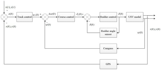
Figure 6. Cascade control used in USV avoidance path point tracking.

The track control loop LOS algorithm as shown in Figure 7 takes two adjacent points $p_k=\left[x_k,y_k\right]$ and $p_{k+1}=\left[x_{k+1},y_{k+1}\right]$ in the collision avoidance path point set $p_n$ into consideration. If at a time point t, the position of the USV is $p_t={[x,y]}^T$, make a circle with $p_t$ as the center and $R$ as the radius to intersect with line segment $\overline{p_k{p}_{k+1}}$ at two points; define the closest point to $p_{k+1}$ of the two points as the target point $p_{los}={[x_{los},y_{los}]}^T$; the azimuth of $p_{los}$ with respect to $p_t$ is the real-time expected heading angle ${\chi }_d$ of the USV; the lateral tracking error of the USV’s current position $P_t$ and the expected collision avoidance path is $e$, the path tangent angle is ${\chi }_p$ and the relative angle is ${\chi }_r$; based on the geometric relationship, the calculation formula of each variable is

$$\begin{array}{c}{(x_{los}-x)}^2+{(y_{los}-y)}^2=R^2\\ \tan ({\alpha }_k)={\displaystyle \frac{y_{k+1}-y_k}{x_{k+1}-x_k}}={\displaystyle \frac{y_{los}-y_k}{x_{los}-x_k}}=const\\ e=-(x-x_k)\sin a_k+(y-y_k)\cos {\alpha }_k\\ {\chi }_d(e)={\chi }_p+{\chi }_r(e)\\ {\chi }_p={\alpha }_k\\ {\chi }_r(e)=\arcsin ({\displaystyle \frac{-e}{R}})\end{array}$$

(19)

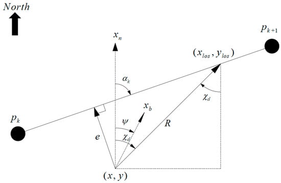
Figure 7. LOS algorithm principle.

In the LOS algorithm, continuously calculating the desired heading angle ${\chi }_d(e)$ to make USV’s heading always directed toward the target point $p_{los}$ ensures that the lateral tracking error $e$ gradually approaches 0, so that the ship can track the planned points.

5. Simulation Studies

USV collision avoidance path planning and tracking simulation experiments have been carried out to verify the superiority of the proposed V-RRT algorithm compared with the classic RRT algorithm. Simulation environment is Microsoft Visual Studio 2017 development environment using C++. The properties of the simulation experiment platform are Intel(R) Core(TM) i7-4720HQ CPU@2.60 GHz with 8 GB of RAM.

‘Mariner’ was taken as the object for simulation tests and main parameters of this ship are shown in Table 1. Chislett et al. (1965) [25] performed systematic PMM tests on it and obtained a number of hydrodynamic derivatives. We took these results to establish non-linear dynamic equation of the ship and carry out tracking tests on this basis. Settings of the main parameters for collision avoidance tests: original course of the ship was north by east 45 degrees. Starting from the coordinate (0, 0), the ship sailed at a constant speed of 15 knots at first. When reaching (3000, 3000), the perception system detected obstacles, and the ship began to prepare for collision avoidance. It was required to complete collision avoidance at (8000, 8000) and resume to original course of the ship. The information of the obstacles is shown in Table 2; the main parameters of planning algorithm and tracking algorithm are set as shown in Table 3.

Table 1. The principal particulars of ‘Mariner’.

Parameter	${\mathit{L}}_{\mathit{O}\mathit{A}}$/m	${\mathit{L}}_{\mathit{p}\mathit{p}}$/m	$\mathit{B}$/m	$\mathit{d}$/m	$\mathit{\Delta }$/t	${\mathit{u}}_{\mathit{o}}$/knots
Value	171.8	160.93	23.17	8.23	19,004.525	15

Table 2. The information of obstacles.

	Coordinate	Radius/m
Obstacle 1	(4000, 1000)	1800
Obstacle 2	(10,500, 6000)	2500
Obstacle 3	(5500, 5500)	2000

Table 3. Parameters used in planning and tracking algorithms.

Parameter	Step-Size S/m	$\mathit{\theta }$/Degree	Radius of LOS Circle/m	${\mathit{K}}_{\mathit{p}}$	${\mathit{T}}_{\mathit{I}}$	${\mathit{T}}_{\mathit{D}}$
Value	2000	60	$abs(error\_dist)+L_{PP}$	1	0	50

5.1. Experimental Results and Analysis in Planning Level

First, we conducted comparative tests on the two algorithms in planning level. As both of the algorithms are substantially randomized algorithms, in order to reduce randomness and increase confidence level, we conducted 10 repeated tests of collision avoidance under same conditions. A comparison of elapsed time of each group of tests is shown in Figure 8a; a comparison of times of child nodes that did not succeed in obstacle detection is shown in Figure 8b; considering restriction of space for the image and for demonstrative purpose, five groups of waypoints were randomly selected from each of the two algorithms, as shown in Figure 9, in which, dotted lines indicate the straight lines connecting two neighboring points rather than represent the actual tracks. Tracking tests of actual tracks will be discussed in Section 5.2 and Section 5.3.

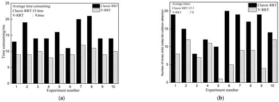
Figure 8. Time consuming comparison (a) and number of times child nodes fail collision detection comparison (b).

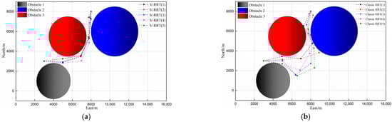
Figure 9. V-RRT collision avoidance path point (a) and classic RRT collision avoidance path point (b).

According to the comparison of distribution of waypoints and based on test results of each group, quantity of waypoints from V-RRT planning is generally less than that with classic RRT. In addition, relative to fluctuation of waypoints in local areas from the classical RRT algorithm, results of V-RRT are smoother; for results of the five groups, planning results from the V-RRT algorithm are more stable and discrepancy among groups is less, while there is significant discrepancy among groups with classic RRT algorithm. The above superiority of the V-RRT algorithm may be ascribed to combined effect of ‘Target attraction vector’ described in Section 4.2 and waypoint corner constraint. ‘Target attraction vector’ may make adjustments towards the target points when extension direction of the search tree is determined to be safe, which allows extension of the search tree to be more purposeful. This may, in addition to increasing stability of the algorithm, compensate to some extent the deficiency of randomness of the classic RRT algorithm and reduce the quantity of the planning points. The waypoint corner constraint may directly impose geometrical restrictions on the connection between neighboring waypoints to prevent a large turning angle and zigzag of the connection line and therefore to improve fluctuation. Meanwhile, by combining a comparison of results as shown in Figure 8b and a distribution of waypoints, it can be seen that relative to the V-RRT algorithm, the distribution of waypoints from classic RRT algorithm in peripheral zones around the obstacles is denser and child nodes that did not succeed in obstacle detection occur more frequently. Such phenomena are due to the design of ‘obstacle repellent vector’ in Section 4.1. This method may provide adjustment away from center of the obstacles when extension direction of the search tree is determined to be dangerous, which allows higher probability that the child nodes are retained and a greater safety margin can be provided to improve safety of the voyage to some extent. The number of failed extension points in the search tree of the V-RRT algorithm is significantly lower than that of the original algorithm, indicating that the sub extension nodes in the iteration process of the V-RRT algorithm have a higher probability of passing the “collision detection”. Accoding to Formula (18), as the reduction in the number of nodes N, the computational complexity has significantly decreased. The combination of the three improvement methods both improves quality of the final waypoints and significantly increases the real-time capability of the algorithm as shown by the comparison results in Figure 8a.

To clarify the statistical reliability of the results, we conducted some calculations to obtain the mean value, Standard Deviation (SD), Confidence Interval (CI), and p-value shown in Table 4.

Table 4. Comparison of time consuming between V-RRT and classic RRT.

Computation time(s)	Mean	SD	95%CI	p-Value
Classic RRT	15.6	3.31	[13.23, 17.97]	3.88 × 10−5
V-RRT	9.6	1.17	[8.76, 10.44]

The p-value calculated through an independent samples t-test is very small (<<0.05), so we can reject the null hypothesis and conclude that there is a significant difference between the means of the two groups. In other words, V-RRT significantly reduces the computational time compared to classic RRT in statistical terms.

5.2. Experimental Results and Analysis in Still Water

Ten groups of waypoints planned by the algorithms before and after improvement were tracked by introducing 3-DOF nonlinear equation of the ship in still water. Final results of statistical comparison of each group of tests are shown in Figure 10. Both tracking strategy and algorithm adopt cascade control and LOS navigation algorithm described in Section 4.4, and control parameters and control laws are identical. From Figure 11, it can be seen that although in the planning level, all planned waypoints of both algorithms fall beyond the obstacle zones as shown by the test results in 5.1, for the final actual course presented by classical RRT algorithm, a number of groups passed through the obstacle zones during tracking simulation tests. According to the statistical results, relative to rate of success in collision avoidance in actual course obtained by classical RRT algorithm, rate of success provided by V-RRT algorithm is 30% higher and reaches 90%. This indicates that in actual application in voyage, the improved algorithm provides higher reliability by significantly reducing both the probability of collision accidents and operation difficulty of the USV. According to Figure 10, navigation time with V-RRT algorithm is far less than that with classic RRT algorithm. Average navigation time with V-RRT algorithm is 2258.5 s and is 22% less than the navigation time of 2890.8 s with the classic RRT algorithm. This implies that with waypoints obtained from the V-RRT algorithm, collision avoidance may be conducted in less time, which implies important significance for the ship with regard to energy saving.

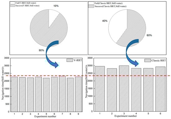
Figure 10. Final results of statistical comparison of each group of tests.

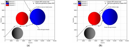
Figure 11. Typical collision avoidance failure path of classic RRT: unable to recover initial course (a), at the collision edge (b).

The results of each group of tests on typical tracking before and after improvement were compared. The two groups of typical actual routes are shown in Figure 12a. Figure 12b–d display comparison of output of rudder angle, resultant velocity, and yaw angle of the two groups of routes. According to performance of the actual routes, the route with the V-RRT algorithm is smoother and may provide a greater safety margin during collision avoidance, while in the route with the classic RRT algorithm, extension direction in local areas is less purposeful and obstacles are brushed past. According to the actual output of the rudder angle, the fairness of waypoints planned with the classic RRT algorithm is relatively lower and the output of the steering engine shows significant fluctuation. As shown by Time Segment 3 in Figure 12a, the rudder angle is changed sharply during this period. This not only expedites the wear of the steering engine but also increases the energy consumption of the ship; meanwhile, as shown by Time Segment 1 and Time Segment 2, the steering engine is with its full rudder, which may increase power consumption of the steering engine. Relatively, when tracking waypoints are obtained from the V-RRT algorithm, only a short duration of full rudder occurs to the steering engine during the overall process, and most of the time, only the small rudder angle is required to complete collision avoidance; according to comparison of resultant velocity U, during the overall process of tracking waypoints obtained from the classic RRT algorithm, there were a number of occasions that the ship stalled severely. As shown by Time segments a in Figure 12c, the velocity of the ship was reduced from 7.25 m/s to 6 m/s and from 7.3 m/s to 5.7 m/s. Based on the theory of ship maneuverability, severe stalling is due to rapid maneuvering and the time coincides with Time Segment 1 and Time Segment 2 in the above result analysis of rudder angle output. This indicates that waypoints planned with classic RRT algorithm bring great difficulty and pressure to control layer to cause drastic motion response of the ship during the overall voyage.

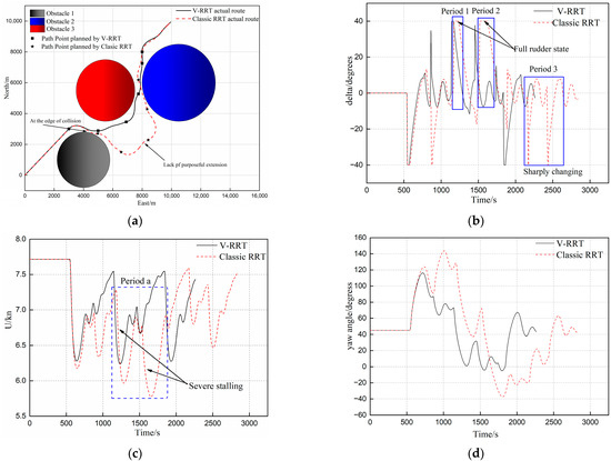
Figure 12. Actual navigation route comparison (a), rudder angle comparison (b), resultant velocity comparison (c), and yaw angle comparison (d).

5.3. Experimental Results and Analysis Considering Ocean Current Load

Ocean currents are horizontal and vertical circulation systems of ocean waters produced by gravity, wind friction, and water density variation in different parts of the ocean. In a relatively short period of time, because the current changes are relatively slow, the flow can be considered constant and uniform during the simulation experiment. In this letter, the current velocity and flow direction in the environment is 1 m/s and 60 degrees.

Similarly to Section 5.1, ten groups of waypoints planned with the algorithms before and after improvement were tracked under current load and identical control parameters and law. Figure 13 displays the comparison of key indicators of actual routes under current load. It can be seen that after current load is introduced, the rate of success in collision avoidance in actual route obtained from the classic RRT algorithm is further reduced from 60% to 40%, and half of them could not return to the pre-set course, while waypoints planned by V-RRT present favorable anti-interference capability and robustness with success rates the same as the success rates in still water.

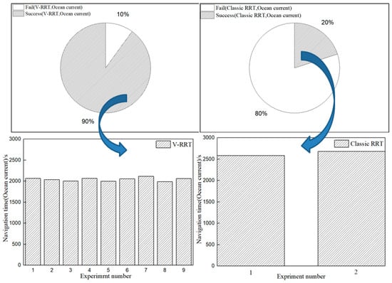
Figure 13. Final results of statistical comparison of each group of tests considering ocean currents.

5.4. Discussion

The simulation results clearly demonstrate the superiority of the V-RRT algorithm over the classic RRT algorithm in terms of both collision avoidance and computational efficiency. However, it is important to consider that the V-RRT algorithm is not without limitations and may occasionally fail under certain conditions.

One of the primary reasons for V-RRT’s occasional failure could be related to the inherent randomness of the algorithm, despite the improvements introduced by the “Target attraction vector” and the “Obstacle repellent vector.” While the algorithm generally performs well in most cases, in highly cluttered or dynamic environments, the random sampling process can occasionally lead to suboptimal path planning, especially when obstacles are densely packed or when there are significant variations in the ship’s speed and maneuverability. This is particularly relevant when the ship’s trajectory deviates significantly from the planned path, as seen in certain failure scenarios.

Additionally, the simplified 3-DOF model used in the simulation excludes critical factors like roll and pitch, potentially affecting the accuracy of the results. While the model is suitable for many scenarios, it may not fully reflect real-world USV dynamics in complex environments. The step-size parameter (S) also plays a crucial role in the performance of the algorithm. Smaller step sizes improve precision but increase computational time, while larger step sizes improve efficiency but may sacrifice path quality. Optimizing this parameter is vital for balancing precision and real-time performance. Lastly, the simulation results highlight the influence of ocean currents on algorithm performance. While the V-RRT algorithm performs well under varying conditions, its robustness in real-world scenarios would benefit from a more accurate model of oceanic forces.

In conclusion, while the V-RRT algorithm shows significant improvements over the classic RRT in terms of collision avoidance, computational efficiency, and robustness, it still faces challenges in highly complex or dynamic environments. The limitations of the 3-DOF model and the influence of the S parameter on performance should be further explored to optimize the algorithm for real-world applications.

6. Conclusions

For issues of collision avoidance of unmanned surface vessel, this paper presents V-RRT algorithm improved based on classic RRT algorithm. Comparison results from simulation tests indicate that waypoints planned with such algorithm show better quality and higher real-time capability; meanwhile, in order to verify feasibility and superiority of waypoints planned with the V-RRT algorithm in actual voyage, a 3-DOF nonlinear dynamic equation of the ship was introduced, and on this basis, the planning results were tracked. Results indicate that success rate with the V-RRT algorithm is higher, navigation time is shorter, and it presents robustness under environmental load. In the future, we plan to (1) continue to optimize EXTEND part based on predictive information about environmental load to further intensify its performance under conditions of broad environmental load; (2) explore the extension of the repellent mechanism to handle multiple collision cones simultaneously; (3) use adaptive parameter tuning techniques, such as reinforcement learning [26] or adaptive control, to dynamically optimize the path planning algorithm; (4) explore to apply the V-RRT algorithm to fleet clusters of USV; (5) conduct tests and the apply the algorithm in practical vessels.

References

- European Maritime Safety Agency. Annual Overview of Marine Casualties and Incidents. 2016. Available online: https://www.emsa.europa.eu/about/financial-regulations/download/4524/2903/23.html (accessed on 10 September 2017).
- Lu, N.; Liu, H.; Wang, Y.; Yan, H. A new real—Time path planning for USV based on dynamic artificial potential field in complex environments. Int. J. Robust Nonlinear Control 2024, 1–17. [Google Scholar] [CrossRef]
- Yang, C.; Pan, J.; Wei, K.; Lu, M.; Jia, S. A novel unmanned surface vehicle path-planning algorithm based on A* and artificial potential field in ocean currents. J. Mar. Sci. Eng. 2024, 12, 285. [Google Scholar] [CrossRef]
- Luan, T.; Tan, Z.; You, B.; Sun, M.; Yao, H. Path planning of unmanned surface vehicle based on artificial potential field approach considering virtual target points. Trans. Inst. Meas. Control 2024, 46, 1190–1202. [Google Scholar] [CrossRef]
- Du, Z.; Li, W.; Shi, G. Multi-USV collaborative obstacle avoidance based on improved velocity obstacle method. ASCE-ASME J. Risk Uncertain. Eng. Syst. Part A Civ. Eng. 2024, 10, 04023049. [Google Scholar] [CrossRef]
- Zhuang, J.; Zhang, Y.; Xu, P.; Zhao, Y.; Luo, J.; Song, S. Multiple moving obstacles avoidance for usv using velocity obstacle method. In Proceedings of the 2021 IEEE International Conference on Unmanned Systems (ICUS), Beijing, China, 15–17 October 2021; pp. 140–145. [Google Scholar]
- Benjamin, M.R.; Curcio, J.A.; Leonard, J.J.; Newman, P.M. Navigation of unmanned marine vehicles in accordance with the rules of the road. In Proceedings of the 2006 IEEE International Conference on Robotics and Automation, Orlando, FL, USA, 15–19 May 2006; IEEE: Piscataway, NJ, USA, 2006; pp. 3581–3587. [Google Scholar]
- Svec, P.; Schwartz, M.; Thakur, A.; Gupta, S.K. Trajectory planning with look-ahead for unmanned sea surface vehicles to handle environmental disturbances. In Proceedings of the 2011 IEEE/RSJ International Conference on Intelligent Robots and Systems, San Francisco, CA, USA, 25–30 September 2011; IEEE: Piscataway, NJ, USA, 2011; pp. 1154–1159. [Google Scholar]
- Wang, H.; Mao, S.; Mou, X.; Zhang, J.; Li, R. Corrigendum: Path planning for unmanned surface vehicles in anchorage areas based on the risk-aware path optimization algorithm. Front. Mar. Sci. 2025, 12, 1584329. [Google Scholar] [CrossRef]
- LaValle, S.M. Rapidly-Exploring Random Trees: A New Tool for Path Planning; The annual research report; Computer Science Department, Iowa State University: Ames, IA, USA, 1998. [Google Scholar]
- Fan, J.; Chen, X.; Liang, X. UAV trajectory planning based on bi-directional APF-RRT* algorithm with goal-biased. Expert Syst. Appl. 2023, 213, 119137. [Google Scholar] [CrossRef]
- Li, Y.; Cui, R.; Li, Z.; Xu, D. Neural Network Approximation Based Near-Optimal Motion Planning with Kinodynamic Constraints Using RRT. IEEE Trans. Ind. Electron. 2018, 65, 8718–8729. [Google Scholar] [CrossRef]
- Huang, T.; Fan, K.; Sun, W. Density gradient-RRT: An improved rapidly exploring random tree algorithm for UAV path planning. Expert Syst. Appl. 2024, 252, 124121. [Google Scholar] [CrossRef]
- Joshua, R.; Jayesh, N.A.; Jovan, D.B. Real-time obstacle detection and reactive path planning system for autonomous small-scale helicopters. In Proceedings of the AIAA Guidance, Navigation and Control Conference and Exhibit, Hilton Head, NC, USA, 20–23 August 2007; AIAA: San Diego, CA, USA, 2007; pp. 1–22. [Google Scholar]
- Martin, S.R.; Wright, S.E.; Sheppard, J.W. Offline and online evolutionary Bi-Directional RRT algorithms for efficient re-planning in dynamic environments. In Proceedings of the 2007 IEEE International Conference on Automation Science and Engineering, Scottsdale, AZ, USA, 22–25 September 2007; IEEE: Piscataway, NJ, USA, 2007; pp. 1131–1136. [Google Scholar]
- Ian, G.; Jonathan, P.H. Improving the efficiency of rapidly-exploring random trees using a potential function planner. In Proceedings of the 44th IEEE Conference on Decision and Control, Seville, Spain, 15 December 2005; IEEE: Piscataway, NJ, USA, 2005; pp. 7965–7970. [Google Scholar]
- Neto, A.A.; Macharet, D.G.; Campos, M.F.M. On the Generation of Trajectories for Multiple UAVs in Environments with Obstacles. J. Intell. Robot. Syst. 2010, 57, 123–141. [Google Scholar] [CrossRef]
- Moon, C.B.; Chung, W. Kinodynamic Planner Dual-Tree RRT (DT-RRT) for Two-Wheeled Mobile Robots Using the Rapidly Exploring Random Tree. IEEE Trans. Ind. Electron. 2014, 62, 1080–1090. [Google Scholar] [CrossRef]
- Yin, G.-Y.; Zhou, S.-L.; Wu, Q.-P. An Improved RRT Algorithm for UAV Path Planning. Acta Electron. Sin. 2017, 45, 1764–1769. [Google Scholar]
- Heo, Y.J.; Chung, W.K. RRT-based path planning with kinematic constraints of AUV in underwater structured environment. In Proceedings of the 2013 10th International Conference on Ubiquitous Robots and Ambient Intelligence (URAI), Jeju, Republic of Korea, 30 October–2 November 2013; IEEE: Piscataway, NJ, USA, 2013. [Google Scholar]
- Chiang, H.T.; Tapia, L. COLREG-RRT: A RRT-based COLREGS-Compliant Motion Planner for Surface Vehicle Navigation. IEEE Robot. Autom. Lett. 2018, 3, 2024–2031. [Google Scholar] [CrossRef]
- Zhuang, J.Y.; Zhang, L.; Sun, H.B.; Su, Y. Improved rapidly-exploring random tree algorithm application in unmanned surface vehicle local path planning. J. Harbin Inst. Technol. 2015, 47, 112–117. [Google Scholar]
- Fossen, T.I. Handbook of Marine Craft Hydrodynamics and Motion Control; John Wiley & Sons: Hoboken, NJ, USA, 2011. [Google Scholar]
- Fiorini, P.; Shiller, Z. Motion planning in dynamic environments using velocity obstacles. Int. J. Robot. Res. 1998, 17, 760–772. [Google Scholar] [CrossRef]
- Chislett, M.; Strom-Tejsen, J. Planar motion mechanism tests and full-scale steering and manoeuvring predictions for a Mariner class vessel. Int. Shipbuild. Prog. 1965, 12, 201–224. [Google Scholar]
- Li, M.; Xu, Z.; Li, S.; Kikuchi, Y.; Dong, Y.; Gryllias, K.C.; Baraldi, P.; Zio, E.; Carroll, J. Health prognostics and maintenance decision-making for wind energy: A comprehensive overview. Renew. Sustain. Energy Rev. 2026, 226, 116269. [Google Scholar] [CrossRef]
Disclaimer/Publisher’s Note: The statements, opinions and data contained in all publications are solely those of the individual author(s) and contributor(s) and not of MDPI and/or the editor(s). MDPI and/or the editor(s) disclaim responsibility for any injury to people or property resulting from any ideas, methods, instructions or products referred to in the content. |
© 2025 by the authors. Licensee MDPI, Basel, Switzerland. This article is an open access article distributed under the terms and conditions of the Creative Commons Attribution (CC BY) license (https://creativecommons.org/licenses/by/4.0/).