ENSO-Modulated Spatio-Temporal Variability of Evaporation Duct Height in the South China Sea

Abstract

The evaporation duct, formed above the ocean surface by sharp vertical gradients of humidity, would significantly influence electromagnetic wave propagation. It is a quasi-permanent feature over the sea, and its strength is quantified by the evaporation duct height (EDH). While previous studies have focused on how local factors influence evaporation ducts, the impact of El Niño–Southern Oscillation (ENSO) on EDH in the South China Sea (SCS) remains undocumented. Using correlation analysis, empirical orthogonal function (EOF) decomposition, and wavelet transform, this study shows that evaporation is the dominant environmental factor controlling EDH variability across seasonal and inter-annual timescales in the SCS, while wind speed and relative humidity play secondary roles with contrasting effects between the northern and southern regions. ENSO drives the inter-annual variability of EDH by modulating evaporation. During El Niño events, anomalous anticyclonic circulations near the Philippine Sea, which weaken (strengthen) the evaporation in the northern (southern) SCS, alter EDH and contribute to the formation of the meridional dipole structure, particularly within the 2-to-6-year ENSO band. These results provide new insights into the mechanisms controlling EDH in the SCS and highlight the critical role of ENSO in shaping its spatial distribution.

1. Introduction

The evaporation duct is a prevalent atmospheric phenomenon that occurs just above the sea surface due to sharp vertical gradients in humidity [1,2,3]. These ducts trap and guide electromagnetic waves, significantly modifying their propagation over the ocean. This affects maritime communication and radar performance, significantly impacting radar detection range and accuracy. The presence of ducts also induces signal fluctuations, which can compromise the reliability and coverage of maritime microwave communications [1,4,5]. The evaporation duct height (EDH) is the most important parameter used to describe the strength of the evaporation duct. It is typically defined as the height of the lowest modified refractivity, M, which is primarily determined by meteorological conditions [4,5,6]. The variability of evaporation ducts is highly complex [3,4], as they are extremely sensitive to hydrological and meteorological conditions at the air–sea interface, such as wind speed (WS), sea-surface temperature (SST), and humidity. Due to the difficulties in directly measuring M, researchers usually use the Monin—Obukhov (M-O) similarity theory in combination with various empirical models, such as the Paulus—Jeske (PJ) model [4,5,6,7], the Musson—Gauthier—Bruth (MGB) model [8], the Babin model [9], and the Naval Postgraduate School (NPS) model [10], to describe the profiles of M, and in turn to deduce the EDH. Under unstable atmospheric conditions, the NPS model is the most widely used model due to its robustness and reliability [10,11,12]. The NPS model outperforms the PJ, MGB and Babin models in comparisons with ocean buoy field data [9]. It also exhibits greater stability than the PJ model [12], and maintains high accuracy under identical atmospheric conditions [13]. The NPS model is considered optimal for estimating modified refractivity profiles [11,14].

Numerous studies have explored the impact of individual meteorological factors on EDH through sensitivity experiments by using reanalysis or observational data [3,15,16,17]. In recent years, several studies have investigated regional EDH evolution by using climatological datasets [18,19,20,21], and revealed notable spatial differences across various oceanic and coastal regions. Previous studies have shown that meteorological factors such as wind speed, air–sea temperature difference, and relative humidity all affect EDH, regardless of atmospheric stability [5,22]. In addition, turbulent fluxes play a crucial role in regulating near-surface atmospheric stability and moisture gradients, thereby exerting a significant influence on the formation and height of evaporation ducts [23].

The South China Sea (SCS), due to its significant strategic importance, strong monsoonal influence, and complex air–sea interactions, has become a critical region for research on EDH. Studies on the diurnal variability, the seasonal evolution, and the spatial distributions of EDH in the SCS [3,4,16,18] have identified that WS, relative humidity (RH), and air–sea temperature difference (ASTD), especially regional evaporation (EVP) [24], are the dominant factors in regulating EDH in summer and winter. However, most existing research focus on short-term or synoptic-scale variations rather than the inter-annual and inter-decadal variability of EDH. As far as we know, the connections between the EDH and regional EVP remain unexplored across seasonal and inter-annual timescales.

The El Niño–Southern Oscillation (ENSO) has a significant impact on atmospheric circulation across the SCS [25,26,27]. ENSO-related anomalies in surface horizontal winds [28,29,30], SST [25,31], and convection [32,33] jointly influence the thermodynamic and dynamic structure of the atmospheric boundary layer, which may in turn influence the characteristics of EDH. However, the mechanism by which ENSO modulates EDH in the SCS remains unclear.

Therefore, the following questions arise: (1) Is there a significant relationship between the EDH and regional EVP at seasonal and inter-annual timescales? and (2) does the ENSO influence EDH, and if so, what are the main pathways? Addressing these questions is crucial for clarifying the mechanisms that link large-scale climate variability to EDH structures.

This paper is organized as follows. After the introduction, Section 2 describes the data and methods. Section 3.1 examines the seasonal and regional characteristics of EDH and evaporation in the SCS, highlighting the seasonal-phase-dependent correlation and pronounced north–south contrasts. It also measures the correlation of EDH with environmental factors in the north and south SCS. Section 3.2 analyzes the inter-annual variability of EDH and its correlation with evaporation in different sub-regions of SCS. Section 3.3 employs wavelet analysis and EOF to identify the dominant time-frequency characteristics and spatial modes of the EDH anomalies, combined with correlation, regression, and wavelet coherence analyses to quantify their linkage. Granger causality testing is then applied to establish the causal direction and optimal lag structure. In this section, we study how ENSO influences the inter-annual variability of EDH by modulating evaporation. Finally, Section 4 summarizes the main conclusions.

2. Data and Methods

2.1. Data

This study utilizes the European Centre for Medium-Range Weather Forecasts (ECMWF) fifth-generation reanalysis (ERA5) monthly data on single levels from 1970 to 2023, with a spatial resolution of 0.25° × 0.25° [34]. The dataset includes air temperature, SST, specific humidity at 2 m, surface wind speed at 10 m, and surface pressure, which are used to calculate the profiles of EDH based on the NPS model. In addition, the evaporation variable is derived from the ERA5 dataset to ensure consistency among all parameters used in the analysis. ERA5 data have been widely used and verified to be suitable for studies on EDH distributions [23,35,36]. Moreover, ERA5 data show stable performance compared with the measured results of meteorological data from weather stations [37] and strong agreement with ship-based measurements [15]. As such, these studies confirm that evaporation duct parameters derived from ERA5 data are reliable.

The classification of ENSO warm and cold phases, known as El Niño and La Niña, respectively, is based on the Oceanic Niño Index (ONI). The ONI is defined as a 3-month running mean SST anomaly in the Niño 3.4 region (5° N–5° S, 120–170° W) that exceeds ±0.5 °C for a minimum of five consecutive overlapping seasons [38]. ONI values are one of the most widely used indices for monitoring and classifying ENSO events [39,40].

2.2. Methods

In this study, the NPS model is used to diagnose the EDH in the SCS. The NPS model identifies the EDH by detecting the altitude corresponding to the minimum M, rather than relying on the traditional ∂M/∂z = 0 criterion used in other models. M can be expressed as follows [22]:

$$M={\displaystyle \frac{77.6P}{T}}-5.6{\displaystyle \frac{e}{T}}+3.75\times {10}^5{\displaystyle \frac{e}{T^2}}+0.157z,$$

(1)

where T (K) is air temperature, P (hPa) represents atmospheric pressure, e (hPa) is partial pressure of water vapor, and z (m) is height above the sea surface.

Through the Tropical Oceans Global Atmosphere—Coupled Ocean-Atmosphere Response Experiment algorithm, the NPS model calculates the temperature and humidity scale parameters by accounting for the effect of salinity on atmospheric humidity [41,42,43]. This modification adopts the advanced air–sea flux algorithm CPARE3.0 and expands the application of the M-O similarity theory to low WS conditions. In the NPS model, the profiles of pressure, potential temperature, and specific humidity are expressed as follows:

$$T\left(z\right)=T\left(z_{0t}\right)+{\displaystyle \frac{{\theta }_{*}}{\kappa }}\left[ln\left({\displaystyle \frac{z}{z_{0t}}}-{\Psi }_h\left({\displaystyle \frac{z}{L}}\right)\right)\right]-{\Gamma }_{d}z,$$

(2)

$$q\left(z\right)=q\left(z_{0q}\right)+{\displaystyle \frac{q_{*}}{\kappa }}\left[ln\left({\displaystyle \frac{z}{z_{0q}}}-{\Psi }_h\left({\displaystyle \frac{z}{L}}\right)\right)\right],$$

(3)

$$P\left(z_2\right)=P\left(z_1\right)exp\left({\displaystyle \frac{g\left(z_1-z_2\right)}{R{\overline{T}}_v}}\right),$$

(4)

$$e={\displaystyle \frac{qp}{\epsilon +\left(1-\epsilon \right)q}},$$

(5)

$${\displaystyle \frac{z}{L}}={\displaystyle \frac{z\kappa g\left[{\theta }_{*}\left(1+0.6078q\right)+0.6078T{q}_{*}\right]}{{\theta }_v{u}_{*}^2}},$$

(6)

$${\overline{T}}_v={\displaystyle \frac{\left[T_v\left(z_1\right)+T_v\left(z_2\right)\right]}{2}},$$

(7)

T(z) and q(z) denote the air temperature and specific humidity at height z, respectively. $\mathrm{P}\left(z_2\right)$ represents the air pressure at height $z_2$.${ \Psi }_h$ is the temperature-specific humidity similarity function, and L is the M-O length. $z_{0t}$ and $z_{0q}$ are the roughness lengths for air temperature and specific humidity, respectively. ${\Gamma }_d$ is the atmospheric dry adiabatic lapse rate. ${\theta }_{*}$, $q_{*}$ and $u_{*}$ are the M-O scaling parameters. $\kappa =0.4$ is the von Kármán constant. ${\overline{T}}_v$ is the mean virtual temperature of the layer between the height $z_1$ and $z_2$. ${ \theta }_v$ is virtual potential temperature, $g$ is the acceleration due to gravity, R is the dry air gas constant, and $\epsilon$ = 0.622 is the ratio of the molecular weight of water vapor to that of dry air.

This study employs the wavelet transform [44,45] to explore the multi-scale time-frequency characteristics of the EDH and evaporation, and therefore to reveal their variation patterns and evolution over different time scales. The EOF is used to analyze the spatial modes and temporal variations in anomalies in EDH. Additionally, cross wavelet spectra and wavelet coherence analyses are employed to investigate the interactions between ENSO and EDH [46,47]. These techniques are widely used in geophysical sciences to identify covariance and coherence in time series [48,49]. The correlation coefficient and regression coefficient are used to measure the relationship between EDH and ENSO. Statistical significance is assessed by using two-tailed Student’s t-tests.

Furthermore, to delve deeper into the relationship between ENSO and EDH, a Granger causality analysis is conducted to examine the propagation lag effects [50,51,52]. For the Granger causality test, five lag periods (1, 2, 3, 4 and 5) are designated. The significance of Granger causality is evaluated through the F-statistic.

3. Results

3.1. The Seasonal Distribution Characteristics of EDH

The distributions of climatological monthly average EDH in the SCS are shown in Figure 1. Seasonal and meridional variations in the EDH, ranging from 5.5 to 18.0 m, are pronounced. In all months, the SCS remains almost exclusively in unstable states, which can be indicated by negative values of the air–sea temperature difference (ΔT = Tair − SST) (Figure S1). High EDH, exceeding 14 m, appears in the northern SCS in October and expands southwards until covering almost the whole SCS in November, December, and January (Figure 1h–k). Then, the EDH decreases progressively from January through March, and the reduction is more marked in the northern SCS than in the southern SCS (Figure 1a,k,l). From March through June, the EDH is progressively and moderately elevated (Figure 1a–d). In contrast to the October–December pattern, this elevation appears first in the southern SCS and expands northwards. The EDH becomes relatively constant at 12 to 13 m in the whole SCS during the summer (June–August, Figure 1d–f). September appears to be a transitional period between summer and October (Figure 1g). The pronounced meridional disparity and significant seasonal variability are characteristic of the EDH in the SCS.

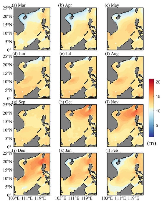
Figure 1. (a–l) Distributions of climatological monthly average evaporation duct height (EDH, unit: m) in the South China Sea (SCS).

The distributions of regional evaporation (Figure 2) follow a similar pattern to the EDH distributions (Figure 1) because both evaporation and EDH are governed by atmospheric conditions and marine environments, which are primarily modulated by the East Asian monsoon. High evaporation, exceeding 7 ${\mathrm{m}\mathrm{m} \mathrm{d}\mathrm{a}\mathrm{y}}^{-1}$, appears in the northern SCS in October, coinciding with the onset of the northeast monsoon, and expands southwards until covering nearly the entire SCS during November to January (Figure 2h–k). This distributional pattern is almost identical with that of EDH, highlighting a strong coupling between EDH and evaporation. Evaporation decreases noticeably in the northwestern SCS as the northeast monsoon weakens from February to May, driving a concurrent decline of EDH in the region (Figure 2a–c,l). During the summer, the EDH increases in response to a moderate increase in evaporation across the basin, especially in the southern SCS (Figure 2d–f). In the inter-monsoonal season in September, evaporation decreases again before it is elevated in October (Figure 2g).

Figure 2. (a–l) Distributions of climatological monthly average evaporation (unit: ${\mathrm{m}\mathrm{m} \mathrm{d}\mathrm{a}\mathrm{y}}^{-1}$) with horizontal winds (vector, unit: m/s) in the SCS. The red boxes show the separated regions used in Figure 3, Figure 4, Figure 5 and Figure 6. Wind directions are shown in the arrow directions, and wind speeds are represented by the scaling of the arrows.

Figure 3. Monthly variations in the correlation coefficients between environment variables and EDH. Solid (northern SCS) and dashed (southern SCS) lines show the correlation coefficients of EDH with EVP, WS, RH, and ASTD in orange, purple, blue, and green, respectively. Black dashed lines show the 99% confidence level.

Figure 4. Climatological monthly average (a) EDH (unit: m) and (b) evaporation (unit: ${\mathrm{m}\mathrm{m} \mathrm{d}\mathrm{a}\mathrm{y}}^{-1}$ ) in the SCS as a whole (black), the northern SCS (red), and the southern SCS (blue). The error bars depict ±1 standard deviation associated with the mean values.

Figure 5. Monthly time series of EDH deviations (unit: m) from 1970 to 2023 for the northern SCS (red), and the southern SCS (blue). The deviations are calculated relative to the climatological monthly means from 1970 to 2023 for the entire SCS (black line in Figure 4a).

Figure 6. Monthly time series of evaporation deviations (unit: ${\mathrm{m}\mathrm{m} \mathrm{d}\mathrm{a}\mathrm{y}}^{-1}$ ) from 1970 to 2023 for the northern SCS (red), and the southern SCS (blue). The deviations are calculated relative to the climatological monthly means from 1970 to 2023 for the entire SCS (black line in Figure 4b).

To examine the north–south contrast in EDH and EVP, the SCS is divided into two sub-regions along 14°N (Figure 2, red boxes). This latitude corresponds to a distinct meridional transition in the climatological distributions of EDH and EVP and coincides with the phase reversal of the first EOF mode of EDH anomalies (Figure 7). The correlation coefficients (r) between environmental variables and EDH are then calculated for each region using monthly data, allowing for an evaluation of their distinct seasonal and regional correlations, as detailed in Figure 3.

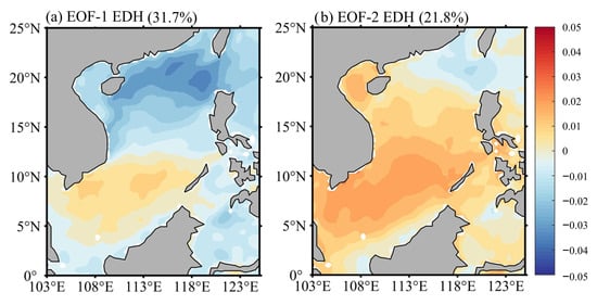
Figure 7. Spatial patterns of (a) EOF-1 and (b) EOF-2 of the EDH anomalies in the SCS. EOF-1 and EOF-2 account for 31.7% and 21.8% of the total variance for EDH deviations, respectively.

The seasonal variation in the EDH over the SCS shows notable regional differences caused by EVP. The EDH in the northern SCS is governed by WS through its control of EVP from November to February, and by RH through its suppression of EVP from March to May. In the southern SCS, the EDH is primarily influenced by RH, with only a minor impact from WS. Evaporation demonstrates the largest positive correlations, ranging from 0.73 to 0.93 in the northern SCS and 0.54 to 0.88 in the southern SCS, establishing it as the primary driver of EDH variability and highlighting the essential role of air–sea heat exchange. The influence of other factors, however, differs significantly between the two regions. In the northern SCS, WS exhibits a significantly stronger correlation with EDH, ranging from 0.35 to 0.81, compared to 0.27 to 0.69 in the south. This supports a co-dominant control mechanism between WS and EVP from November to February. From March to May, RH emerges as a key constraining factor in both regions, with r peaking at –0.80 in the north and –0.76 in the south. In the southern SCS, RH shows a strong negative correlation with EDH throughout the year, ranging from −0.42 to −0.76, while the correlation for WS is highly fluctuating and generally weak. This may be because RH has higher values in the south than in the north, making RH the main factor of EVP. ASTD shows the weakest correlation, confirming a lower thermal sensitivity of EDH in the southern sector.

The climatological monthly average EDH and evaporation in the entire SCS as a whole, as well as in the northern and southern SCS, are shown in Figure 4. Seasonal variations in EDH and evaporation both exhibit a distinct bimodal pattern. The annual average EDH in the SCS as a whole is about 12.3 m. The maximum monthly EDH of 13.1 m is found in December when the northeast monsoon prevails. In addition to the winter maximum, there is also a summer maximum, with the EDH of 12.5 m, in July during the southwest monsoonal season. The EDH seasonal cycle is marked by two minima, occurring in March and September. Although the seasonal changes in the EDH in the northern SCS and in the southern SCS both follow a similar pattern to that in the SCS as a whole, the EDH in the northern SCS is markedly larger (lower) than in the southern SCS during the northeast (southwest) monsoonal season (Figure 4a). The seasonal evolution of evaporation, with peaks in December and July and troughs in April and September, follows a pattern similar to that of the EDH (Figure 4b). The standard deviations of the monthly averages range from ±0.34 to ±0.61 m for EDH and from ±0.24 to ±0.73 mm day⁻¹ for evaporation. These values are substantially smaller than the magnitudes of the seasonal cycle, indicating that seasonal variability dominates over interannual variations.

3.2. Inter-Annual Variation Characteristics of EDH

The spatial and temporal variations in the monthly EDH deviations are demonstrated through a time-series analysis of their distributions in the northern and southern sub-regions of the SCS (Figure 5). A significant north–south difference, with generally higher EDH from October to January but lower EDH from March to August in the northern SCS, is observed. The difference is most pronounced from October to December, followed by April to June, but not apparent in February and September. Such seasonal and spatial differences in the EDH may reflect the spatial and temporal differences in the effects of seasonal monsoons on the SCS.

To better understand the drivers of the inter-annual variability in EDH, time-series distributions of monthly evaporation deviations (Figure 6) are compared. Evaporation deviations also show an apparent north–south difference. It is larger in the northern SCS than in the southern SCS from October to January. During this period, strong northeast winds, accompanied by dry air, enhance both evaporation and EDH. The influence decreases southwards, resulting in lower evaporation and EDH in the southern SCS. From March to May, associated with the weakening of the northeast monsoons, evaporation is progressively reduced from the north to the south. Correspondingly, the EDH is moderately reduced in the northern SCS. From June through August, attributed to the prevailing southwest monsoons, evaporation and EDH are larger in the southern SCS.

The above results highlight that evaporation is the primary driver of both seasonal and inter-annual EDH variability. Enhanced evaporation increases moisture loss and reduces near-surface humidity, thereby steepening the vertical moisture gradient and elevating the EDH. This mechanism is consistent with previous reports that the M-gradient is primarily associated with humidity gradients under unstable atmospheric conditions [23,53].

3.3. Modes of Evaporation Duct and Its Relations with ENSO

Before conducting the EOF analysis, the seasonal cycle was removed. First, each EDH value was subtracted by the climatological monthly mean in the corresponding month. Then, a 13-point running mean was applied to the generated EDH deviations to smooth high-frequency noise. As such, the EOF modes presented in the paper reflect inter-annual to decadal variability, with the seasonal component effectively removed [54,55,56,57]. The first two EOF modes, EOF-1 and EOF-2, account for 31.7% and 21.8% of the total variance for anomalies of EDH, respectively. EOF-1 and EOF-2 are well separated from each other [58].

The EOF analysis identifies two distinct modes of EDH variability over the SCS. The leading mode (EOF-1) shows a pronounced meridional dipole structure and is strongly linked to ENSO, while the second mode (EOF-2) displays a weaker and temporally evolving connection. Specifically, the EOF-1 spatial pattern is characterized by a south-to-north “positive–negative” dipole, with a negative center west of the Luzon Strait and a positive center off the eastern coast of Vietnam (Figure 7a). The corresponding first principal component (PC-1) time series (Figure 8a) is significantly positively correlated with the ONI (r = 0.63; p < 0.01), indicating that ENSO is a dominant driver accounting for the inter-annual variability in the EDH. For instance, from May 1973 to April 1976, during a La Niña event, PC-1 was all negative. In the months of April 1982 to June 1983, and May 1997 to May 1998, when ENSO occurred, PC-1 was positive.

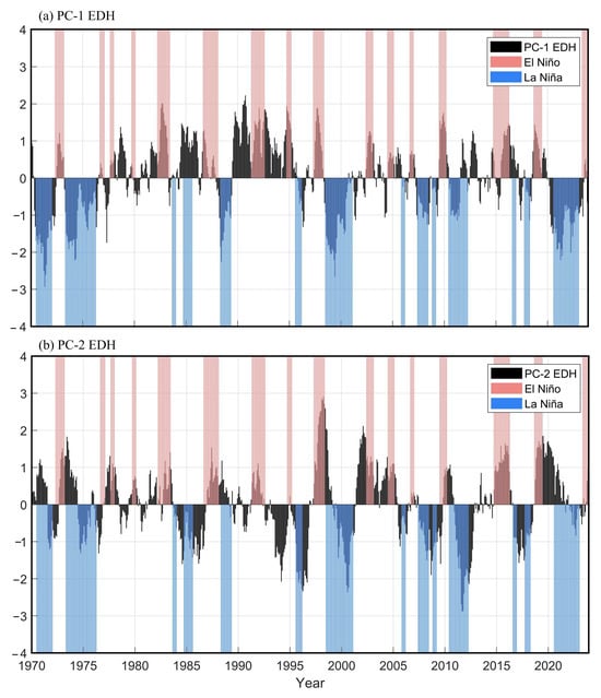
Figure 8. Time series for the normalized principal components (black bars) of (a) PC-1 and (b) PC-2. The El Niño and La Niña events, based on the ONI, are shown in the red and blue bars, respectively.

The EOF-2 is characterized by a southwest–northeast dipole pattern with the negative values of EOF-2 found west of the Luzon Strait, and the positive center occurring in a further south-west area than that of EOF-1 (Figure 7b). The PC-2 has a weak correlation (r = 0.38) with the ONI (Figure 8b). For instance, a phase discrepancy between the ONI and PC-1 is evident during the period from May 1973 to April 1976. Actually, the correlation is very weak prior to 2000 (r = 0.22), but r rises to 0.56 after 2000. This suggests a strengthened influence of ENSO on EDH in recent decades. Nevertheless, the interpretation of EOF-2 is complex and beyond the scope of this study.

The primary timescale of EDH variability, based on wavelet transform analyses of the PC-1 of the EDH anomalies, lies in the 2 to 6 years band (Figure 9). This timescale is particularly evident from 1985 to 2002 and 2008 to 2020. Given that the typical timescale of ENSO events ranges from 2 to 7 years [26,59,60], the inter-annual variability of the EDH is likely influenced by ENSO. In addition to this primary timescale, an inter-decadal variability in the EDH, with a period of 9 to 16 years, has also been observed since 1985. The potential modulation by the Pacific Decadal Oscillation (PDO) warrants future investigation.

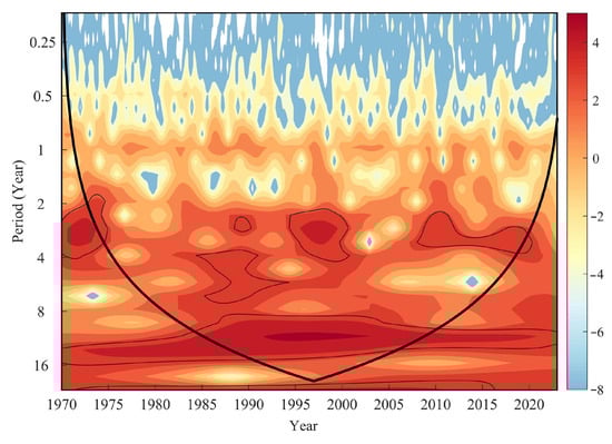
Figure 9. Continuous Morlet wavelet spectrum of the normalized time series of the EOF-1 modes for the EDH anomalies in the SCS. The thin contours depict the 95% confidence level of local power relative to a white noise background. Thin contours denote the 95% confidence level for significant wavelet power, and the thick line defines the cone of influence, bounding the region unaffected by zero-padding artifacts.

To further verify this linkage and quantify the time–frequency coherence between ENSO and EDH variability, we conducted cross-wavelet and wavelet coherence analyses between ONI and PC-1. ONI and PC-1 demonstrate sustained, stable, and significant common power as well as linear correlation within the 2-to-5-year cycle band. The 2-to-5-year cycle band persists throughout nearly the entire period from 1970 to 2023 and has passed the 95% confidence test, indicating the concurrent occurrence of strong ENSO and PC1 signals in this band. Scattered significant regions are also observed in the 0.5–1 year cycle band. However, these regions have short duration and small area, resulting in low statistical reliability (Figure 10a). The wavelet coherence values corresponding to the 2–5-year band exhibit high energy and strong linear correlation during the period 1982–2023. Within the significant regions of the 2-to-5-year band, the phase arrows generally point downward to the right, implying that ENSO leads PC-1 (Figure 10b).

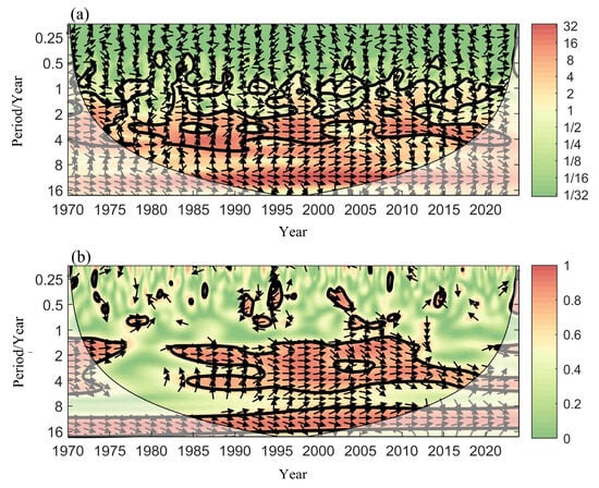
Figure 10. Cross-wavelet spectrum (a) and wavelet coherency (b) analysis showing the relations between ONI and PC-1. The thick black contour indicates the 95% confidence level against red noise and the cone of influence is shown as the lighter shade. The arrows (vectors) designate the phase difference (right for in-phase and left for anti-phase).

ENSO may modulate the EDH through its influences on sea surface horizontal wind and evaporation. As shown in Figure 11, prevailing easterly winds cover most of the SCS under climatological conditions. During El Niño events, anomalous warming in the eastern equatorial Pacific weakens the Walker circulation, which in turn induces an anomalous anticyclonic circulation near the Philippine Sea [29,60] (thick black arrows in Figure 11). Consequently, the easterly winds are weakened (strengthened) in the northern (southern) SCS, resulting in a decrease (increase) of evaporation in the northern (southern) SCS. Since evaporation is a primary driver of EDH, El Niño-induced evaporation changes reduce (elevate) EDH in the northern (southern) SCS, contributing to the formation of the meridional dipole pattern in EDH anomalies.

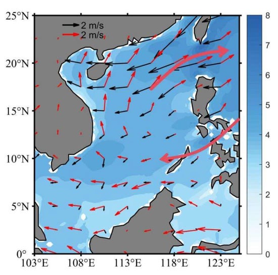
Figure 11. Climatological distributions of evaporation (shaded, unit: ${\mathrm{m}\mathrm{m} \mathrm{d}\mathrm{a}\mathrm{y}}^{-1}$ ), surface wind vectors (black arrows; unit: m/s), and anomalous surface wind vectors (red arrows; unit: m/s) during ENSO events. Thick red arrows show the schematic anticyclonic circulation.

The distributional patterns of the regression coefficients between the ONI and the EDH anomalies and between the ONI and the evaporation anomalies (Figure 12) further confirm the above hypothesis. For both anomalies of EDH and evaporation, negative regression coefficients are found in the northern SCS, while positive regression coefficients are found in the southern SCS.

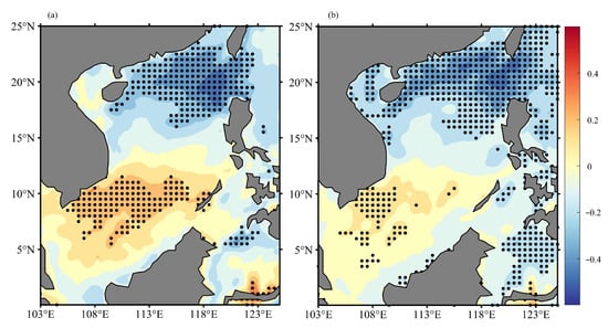
Figure 12. Temporal regression coefficients between ONI and anomalies for (a) EDH and (b) evaporation over SCS, the black dotted area indicates statistically significant coefficients at the 99% confidence level.

Granger causality analysis further reveals a significant causal relationship between ONI and PC-1, indicating that ENSO activity is an important driver of EDH anomalies. The strength of this causal linkage exhibits distinct temporal characteristics, with the strongest causal effect observed at the first lag order, where the F statistic reaches 20.24 and p < 0.05, reflecting a rapid atmospheric response process. As the lag order increases, the F decreases systematically with values of 12.32, 10.96, 10.96 and 9.16 at lag orders of 2, 3, 4 and 5, respectively. This pattern demonstrates that ENSO has predictive value for subsequent duct variations, with the strongest relationship at a one-month lag.

Figure 13 summarizes the dynamic mechanism behind the meridional dipole structure of EDH over the SCS during El Niño events. During El Niño, anomalous warming in the eastern equatorial Pacific weakens the Walker circulation, which in turn induces an anomalous anticyclone over the western North Pacific near the Philippines, as shown by the blue ellipse. This anomalous anticyclone influences the surface wind field over the SCS, weakening the prevailing northeast winds in the northern SCS while strengthening them in the southern part, as shown by the black arrows. The weakened (strengthened) surface winds induced by the anomalous anticyclone lead to a decrease (increase) in latent heat flux and moisture extraction from the sea surface, thereby decreasing (increasing) near-surface evaporation [54], weakening (steepening) the vertical humidity gradient, and ultimately producing lower (higher) EDH in the northern (southern) SCS. These responses in evaporation and humidity stratification form a pronounced meridional dipole of EDH during El Niño events. In conclusion, ENSO alters large-scale atmosphere circulation, leading to boundary-layer wind and humidity changes that modify evaporation and produce regional EDH anomalies across the SCS.

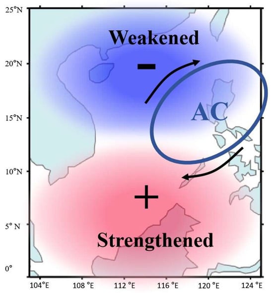
Figure 13. Schematic diagram of the mechanism for the SCS evaporation duct dipole structure. The blue ellipse indicates the schematic anomalous anticyclone, black arrows show schematic wind anomalies, red shading indicates reduced EDH, and blue shading indicates enhanced EDH.

4. Conclusions and Discussion

The evaporation duct is a common phenomenon in marine environments, playing a crucial role in maritime communication and radar detection [9]. The evaporation is the process by which water molecules change from liquid to gas at the sea–air interface. While both EDH and evaporation are key variables in marine boundary layer processes, they represent distinct physical quantities. This study investigates the seasonal evolution and inter-annual variability of EDH over the SCS from 1970 to 2023, highlighting the dominant roles of the ENSO and evaporation in controlling the distributional patterns of the EDH. Results show that EDH exhibits significant seasonal variation, with greater seasonal changes in the northern SCS compared to the southern SCS due to larger fluctuations in evaporation (EVP). Across the SCS, EDH variability is mainly governed by EVP, while the influences of wind speed and relative humidity are secondary and show contrasting regional characteristics between the northern and southern regions. Correlation analysis and spatial comparisons confirm that evaporation influences EDH at seasonal and inter-annual scales, particularly in regulating the meridional dipole structure captured by the EOF-1 mode. Wavelet transform and regression analyses indicate that the temporal variability of EDH is strongly modulated by ENSO, as the dominant inter-annual band of 2 to 6 years agrees well with the typical ENSO cycles. The first principal component time series of the anomalies of EDH displays strong positive correlations with the Oceanic Niño Index, further confirming the role of the ENSO in modulating the inter-annual variability of EDH. ENSO-related anomalous anti-cyclonic circulations near the Philippine Sea modulate EDH by weakening evaporation in the north and enhancing it in the south, contributing to the formation of the meridional dipole pattern captured by the EOF-1 model.

Although our current study provides some new insights into the causes and mechanisms of EDH by focusing on the SCS, further research is needed. First, cross-validation using in situ data from ocean buoys and radiosondes is essential to verify the results [23,61,62]. Second, the inter-decadal signals in EDH may reflect modulation by large-scale modes, such as the Pacific Decadal Oscillation [2,63,64,65], which influence the long-term environmental changes in the SCS. Thirdly, examining how sub-seasonal processes, such as the Madden Julian Oscillation [66,67,68], interact with the ENSO-related environment could enhance the understanding and prediction of EDH under compound climate influences. Finally, the M-O similarity framework offers a fundamental theoretical basis for interpreting how atmospheric stability regulates EDH. Integrating a full set of M-O diagnostic analyses would therefore provide deeper mechanistic insight into the pathways through which ENSO forcing shapes EDH variability.

References

- Anderson, K.D. Radar measurements at 16.5 GHz in the oceanic evaporation duct. IEEE Trans. Antennas Propag. 2002, 3, 100–106. [Google Scholar] [CrossRef]
- Shi, Y.; Zhang, Q.; Wang, S.; Yang, K.; Ma, Y. Impact of Typhoon on Evaporation Duct in the Northwest Pacific Ocean. IEEE Access 2019, 7, 109111–109119. [Google Scholar] [CrossRef]
- Hu, D.; Yang, K.; Zhang, H.; Wang, S.; Yang, F.; Dong, G.; Shi, Y. Observed diurnal variations of over-the-horizon propagation loss in evaporation duct over the South China Sea. IEEE Antennas Wirel. Propag. Lett. 2023, 23, 1060–1064. [Google Scholar] [CrossRef]
- Yang, N.; Song, D.; Lu, T.; Su, D.; Wang, T. The Evaporation Duct Characteristics of Typhoon Kompasu (202118) Based on Buoys Observation. IEEE Antennas Wirel. Propag. Lett. 2024, 24, 212–216. [Google Scholar] [CrossRef]
- Zhang, Q.; Yang, K.; Yang, Q. Statistical analysis of the quantified relationship between evaporation duct and oceanic evaporation for unstable conditions. J. Atmos. Ocean. Technol. 2017, 34, 2489–2497. [Google Scholar] [CrossRef]
- Geernaert, G.L. On the Evaporation Duct for Inhomogeneous Conditions in Coastal Regions. J. Appl. Meteorol. Climatol. 2007, 46, 538–543. [Google Scholar] [CrossRef]
- Ivanov, V.K.; Shalyapin, V.N.; Levadnyi, Y.V. Determination of the Evaporation Duct Height from Standard Meteorological Data. Izv. Atmos. Ocean. Phys. 2007, 43, 36–44. [Google Scholar] [CrossRef]
- Musson-Genon, L.; Gauthier, S.; Bruth, E. A simple method to determine evaporation duct height in the sea surface boundary layer. Radio Sci. 1992, 27, 635–644. [Google Scholar] [CrossRef]
- Babin, S.M.; Young, G.S.; Carton, J.A. A new model of the oceanic evaporation duct. J. Appl. Meteorol. Climatol. 1997, 36, 193–204. [Google Scholar] [CrossRef]
- Frederickson, A.P.; Davidson, K.L.; Goroch, K.A. Operational Bulk Evaporation Duct Model for MORIAH; Naval Postgraduate School: Monterey, CA, USA, 2000; pp. 10–25. [Google Scholar]
- Gunashekar, S.D.; Warrington, E.M.; Siddle, D.R. Long-term statistics related to evaporation duct propagation of 2 GHz radio waves in the English Channel. Radio Sci. 2010, 45, 1–14. [Google Scholar] [CrossRef]
- Yang, S.; Li, X.; Wu, C.; He, X.; Zhong, Y. Application of the PJ and NPS evaporation duct models over the South China Sea (SCS) in winter. PLoS ONE 2017, 12, e0172284. [Google Scholar] [CrossRef]
- Qiu, Z.J.; Zhang, C.; Wang, B.; Hu, T.; Zou, J.; Li, Z.Q.; Chen, S.Z.; Wu, S. Analysis of the accuracy of using ERA5 reanalysis data for diagnosis of evaporation ducts in the East China Sea. Front. Mar. Sci. 2023, 9, 1108600. [Google Scholar] [CrossRef]
- Frederickson, P.A.; Murphree, J.T.; Twigg, K.L.; Barrios, A. A modern global evaporation duct climatology. In Proceedings of the 2008 International Conference on Radar, Adelaide, Australia, 2–5 September 2008; IEEE: Piscataway, NJ, USA, 2008; pp. 292–296. [Google Scholar] [CrossRef]
- Guo, X.; Li, Q.; Zhao, Q.; Kang, S.; Wei, Y.; Yang, L. A comparative study of rough sea surface and evaporation duct models on radio wave propagation. IEEE Trans. Antennas Propag. 2023, 71, 6060–6071. [Google Scholar] [CrossRef]
- Shi, Y.; Yang, K.; Yang, Y.; Ma, Y. A new evaporation duct climatology over the South China Sea. J. Meteorol. Res. 2015, 29, 764–778. [Google Scholar] [CrossRef]
- Tian, B.; Liu, Q.; Lu, J.; He, X.; Zeng, G.; Teng, L. The influence of seasonal and nonreciprocal evaporation duct on electromagnetic wave propagation in the Gulf of Aden. Results Phy. 2020, 18, 103181. [Google Scholar] [CrossRef]
- McKeon, B.D. Climate Analysis of Evaporation Ducts in the South China Sea. Master’s Thesis, Naval Postgraduate School, Monterey, CA, USA, 2013. [Google Scholar]
- Zhang, Q.; Zhu, D.; Liu, C.; Guo, X.; Li, Q.; Yang, L. Research on the Inhomogeneity of Evaporation Duct in the South China Sea Based on the ERA5 Data. In Proceedings of the 2024 Cross Strait Radio Science and Wireless Technology Conference, Macao, China, 4–7 November 2024; IEEE: Piscataway, NJ, USA, 2024; pp. 1–3. [Google Scholar] [CrossRef]
- Sirkova, I. Duct occurrence and characteristics for Bulgarian Black Sea shore derived from ECMWF data. J. Atmos. Sol.-Terr. Phys. 2015, 135, 107–117. [Google Scholar] [CrossRef]
- Zhang, Q.; Yang, K.; Shi, Y. Spatial and temporal variability of the evaporation duct in the Gulf of Aden. Tellus 2016, 68, 29792. [Google Scholar] [CrossRef]
- Brooks, I.M. Air-sea interaction and spatial variability of the surface evaporation duct in a coastal environment. Geophys. Res. Lett. 2001, 28, 2009–2012. [Google Scholar] [CrossRef]
- Franklin, K.B.; Wang, Q.; Jiang, Q.; Shen, L. Understanding evaporation duct variabilities on turbulent eddy scales. J. Geophys. Res. Atmos. 2022, 127, e2022JD036434. [Google Scholar] [CrossRef]
- Yang, K.; Zhang, Q.; Shi, Y. Interannual variability of the evaporation duct over the South China Sea and its relations with regional evaporation. J. Geophys. Res. Ocean. 2017, 122, 6698–6713. [Google Scholar] [CrossRef]
- Latif, M.; Anderson, D.; Barnett, T.; Cane, M.; Kleeman, R.; Leetmaa, A.; O’Brien, J.; Rosati, A.; Schneider, E. A review of the predictability and prediction of ENSO. J. Geophys. Res. Ocean. 1998, 103, 14375–14393. [Google Scholar] [CrossRef]
- McPhaden, M.J.; Zebiak, S.E.; Glantz, M.H. ENSO as an integrating concept in earth science. Science 2006, 314, 1740–1745. [Google Scholar] [CrossRef]
- Tang, Y.; Zhang, R.; Liu, T.; Duan, W.; Yang, D.; Zheng, F.; Ren, H.; Lian, T.; Gao, C.; Chen, D. Progress in ENSO prediction and predictability study. Natl. Sci. Rev. 2018, 5, 826–839. [Google Scholar] [CrossRef]
- McGregor, S.; Ramesh, N.; Spence, P.; England, M.H.; McPhaden, M.J.; Santoso, A. Meridional movement of wind anomalies during ENSO events and their role in event termination. Geophys. Res. Lett. 2013, 40, 749–754. [Google Scholar] [CrossRef]
- Wang, B.; An, S. A mechanism for decadal changes of ENSO behavior: Roles of background wind changes. Clim. Dyn. 2002, 18, 475–486. [Google Scholar] [CrossRef]
- Watanabe, M.; Jin, F.F. Role of Indian Ocean warming in the development of Philippine Sea anticyclone during ENSO. Geophys. Res. Lett. 2002, 29, 111–116. [Google Scholar] [CrossRef]
- Nagura, M.; Konda, M. The seasonal development of an SST anomaly in the Indian Ocean and its relationship to ENSO. J. Clim. 2007, 20, 38–52. [Google Scholar] [CrossRef]
- Lyon, B.; Camargo, S.J. The seasonally-varying influence of ENSO on rainfall and tropical cyclone activity in the Philippines. Clim. Dyn. 2009, 32, 125–141. [Google Scholar] [CrossRef]
- Park, C.H.; Son, S.W. Subseasonal variability of ENSO–East Asia teleconnections driven by tropical convection over the Indian ocean and Maritime Continent. Geophys. Res. Lett. 2024, 51, e2023GL108062. [Google Scholar] [CrossRef]
- Hersbach, H.; Bell, B.; Berrisford, P.; Biavati, G.; Horányi, A.; Muñoz Sabater, J.; Nicolas, J.; Peubey, C.; Radu, R.; Rozum, I.; et al. ERA5 Monthly Averaged Data on Single Levels from 1940 to Present; Copernicus Climate Change Service: Reading, UK, 2023. [Google Scholar] [CrossRef]
- Huang, L.; Zhao, X.; Liu, Y.; Yang, P.; Ding, J.; Zhou, Z. The diurnal variation of the evaporation duct height and its relationship with environmental variables in the South China Sea. IEEE Trans. Antennas Propag. 2022, 70, 10865–10875. [Google Scholar] [CrossRef]
- Wang, S.; Yang, K.; Shi, Y.; Yang, F.; Zhang, H. Impact of evaporation duct on electromagnetic wave propagation during a typhoon. J. Ocean Univ. 2022, 21, 1069–1083. [Google Scholar] [CrossRef]
- Wang, S.; Yang, K.; Shi, Y.; Yang, F. Observations of anomalous over-the-horizon propagation in the evaporation duct induced by Typhoon Kompasu. IEEE Antennas Wirel. Propag. Lett. 2022, 21, 963–967. [Google Scholar] [CrossRef]
- Climate Prediction Center. Oceanic Niño Index. National Centers for Environmental Prediction. 2018. Available online: https://www.climate.gov/news-features/understanding-climate/climate-variability-oceanic-nino-index (accessed on 20 November 2025).
- Hurley, J.V.; Vuille, M.; Hardy, D.R. On the interpretation of the ENSO signal embedded in the stable isotopic composition of Quelccaya Ice Cap, Peru. J. Geophys. Res. Atmos. 2019, 124, 6644–6661. [Google Scholar] [CrossRef]
- Sylvia, C.; Sullivan, K.A.; Schiro, K.A.; Gentine, P. The Response of Tropical Organized Convection to El Niño Warming. J. Geophys. Res. Atmos. 2019, 124, 8481–8500. [Google Scholar] [CrossRef]
- Babin, S.M.; Dockery, G.D. LKB-based evaporation duct model comparison with buoy data. J. Appl. Meteorol. Clim. 2002, 41, 434–446. [Google Scholar] [CrossRef]
- Burk, S.D.; Haack, T.; Rogers, L.T.; Wagner, L.J. Island Wake Dynamics and Wake Influence on the Evaporation Duct and Radar Propagation. J. Appl. Meteorol. Clim. 2003, 42, 349–367. [Google Scholar] [CrossRef]
- Newton, D.A. Coamps Modeled Surface Layer Refractivity in the Roughness and Evaporation Duct Experiment 2001. Master’s Thesis, Naval Postgraduate School, Monterey, CA, USA, 2003. [Google Scholar]
- Markovic, D.; Koch, M. Wavelet and scaling analysis of monthly precipitation extremes in Germany in the 20th century: Interannual to interdecadal oscillations and the North Atlantic Oscillation influence. Water Resour. Res. 2005, 41, W09420. [Google Scholar] [CrossRef]
- Torrence, C.; Compo, G.P. A practical guide to wavelet analysis. Bull. Am. Meteorol. Soc. 1998, 79, 61–78. [Google Scholar] [CrossRef]
- Grinsted, A.; Moore, J.C.; Jevrejeva, S. Application of the cross wavelet transform and wavelet coherence to geophysical time series. Nonlinear Process. Geophys. 2004, 11, 561–566. [Google Scholar] [CrossRef]
- Jevrejeva, S.; Moore, J.C.; Grinsted, A. Influence of the Arctic Oscillation and El Niño-Southern Oscillation (ENSO) on ice conditions in the Baltic Sea: The wavelet approach. Geophys. Res. Atmos. 2003, 108, 4677. [Google Scholar] [CrossRef]
- Baddoo, T.D.; Guan, Y.; Zhang, D.; Andam-Akorful, S.A. Rainfall variability in the Huangfuchuang watershed and its relationship with ENSO. Water 2015, 7, 3243–3262. [Google Scholar] [CrossRef]
- Baddoo, T.D.; Guan, Y.; Zhang, D.; Andam-Akorful, S.A.; Shanahan, T.M.; Overpeck, J.T.; Anchukaitis, K.J.; Beck, J.W.; Cole, J.E.; Dettman, D.L.; et al. Atlantic forcing of persistent drought in West Africa. Science 2009, 324, 377–380. [Google Scholar] [CrossRef]
- Granger, C.W.J. Investigating causal relations by econometric models and cross-spectral methods. Econometrica 1969, 37, 424–438. [Google Scholar] [CrossRef]
- Xie, X.; He, B.; Guo, L.; Miao, C.; Zhang, Y. Detecting hotspots of interactions between vegetation greenness and terrestrial water storage using satellite observations. Remote Sens. Environ. 2019, 231, 12. [Google Scholar] [CrossRef]
- Sun, K.; Yang, P.; Xia, J.; Huang, H.; Chen, Y.; Zhu, Y.; Wang, C.; Yao, P.; Chen, L.; Song, J.; et al. Spatiotemporal correlations and driving factors of multiple drought in Central Asia. Atmos. Res. 2025, 324, 108199. [Google Scholar] [CrossRef]
- Cook, J. A sensitivity study of weather data inaccuracies on evaporation duct height algorithms. Radio Sci. 1991, 26, 731–746. [Google Scholar] [CrossRef]
- Xie, S.P.; Philander, S.G.H. A coupled ocean-atmosphere model of relevance to the ITCZ in the eastern Pacific. Tellus 1994, 46, 340–350. [Google Scholar] [CrossRef]
- Moten, S. Multiple time scales in rainfall variability. Proc. Indian Acad. Sci.—Earth Planet. Sci. 1993, 102, 249–263. [Google Scholar] [CrossRef]
- Zhao, J.; Cao, Y.; Shi, J. Core region of Arctic Oscillation and the main atmospheric events impact on the Arctic. Geophys. Res. Lett. 2006, 33, L22708. [Google Scholar] [CrossRef]
- Zhao, J.; Cao, Y.; Shi, J. Spatial variation of the arctic oscillation and its long-term change. Tellus 2010, 62A, 661–672. [Google Scholar] [CrossRef]
- North, G.R.; Bell, T.L.; Cahalan, R.F.; Moeng, F.J. Sampling errors in the estimation of empirical orthogonal functions. Mon. Weather Rev. 1982, 110, 699–706. [Google Scholar] [CrossRef]
- Santoso, A.; McPhaden, M.J.; Cai, W. The defining characteristics of ENSO extremes and the strong 2015/2016 El Niño. Rev. Geophys. 2017, 55, 1079–1129. [Google Scholar] [CrossRef]
- Kim, J.; An, S.; Jun, S.; Park, H.; Yeh, S. ENSO and East Asian winter monsoon relationship modulation associated with the anomalous northwest Pacific anticyclone. Clim. Dyn. 2017, 49, 1157–1179. [Google Scholar] [CrossRef]
- Chiao, M.; Hou, J.; Pien, K. A study of evaporation duct characteristics in the South China Sea during the Winter of 2017. Atmos. Res. 2024, 304, 107356. [Google Scholar] [CrossRef]
- Yang, F.; Wang, S.; Yang, K.; Shu, Y.; Shi, Y. Marine high—Speed over—The—Horizon communications and channel sensing in evaporation ducts over the South China Sea. IEEE Antennas Wirel. Propag. Lett. 2024, 23, 2870–2874. [Google Scholar] [CrossRef]
- Cheng, X.; Xie, S.; Du, Y.; Wang, J.; Chen, X.; Wang, J. Interannual-to-decadal variability and trends of sea level in the South China Sea. Clim. Dyn. 2016, 46, 3113–3126. [Google Scholar] [CrossRef]
- Xu, M.; Xu, H.; Ma, J.; Deng, J. Impact of Pacific Decadal Oscillation on interannual relationship between El Niño and South China Sea summer monsoon onset. Int. J. Climatol. 2022, 42, 2739–2753. [Google Scholar] [CrossRef]
- Xue, X.; Chen, W.; Chen, S.; Feng, J. PDO modulation of the ENSO impact on the summer South Asian high. Clim. Dyn. 2018, 50, 1393–1411. [Google Scholar] [CrossRef]
- Maloney, E.D.; Kiehl, J.T. MJO-related SST variations over the tropical eastern Pacific during Northern Hemisphere summer. J. Clim. 2002, 15, 675–689. [Google Scholar] [CrossRef]
- Tong, H.W.; Chan, J.C.; Zhou, W. The role of MJO and mid-latitude fronts in the South China Sea summer monsoon onset. Clim. Dyn. 2009, 33, 827–841. [Google Scholar] [CrossRef]
- Wang, G.; Ling, Z.; Wu, R.; Chen, C. Impacts of the Madden–Julian oscillation on the summer South China Sea ocean circulation and temperature. J. Clim. 2013, 26, 8084–8096. [Google Scholar] [CrossRef]
Disclaimer/Publisher’s Note: The statements, opinions and data contained in all publications are solely those of the individual author(s) and contributor(s) and not of MDPI and/or the editor(s). MDPI and/or the editor(s) disclaim responsibility for any injury to people or property resulting from any ideas, methods, instructions or products referred to in the content. |
© 2025 by the authors. Licensee MDPI, Basel, Switzerland. This article is an open access article distributed under the terms and conditions of the Creative Commons Attribution (CC BY) license (https://creativecommons.org/licenses/by/4.0/).