Abstract
Artificial neural networks have been evaluated and compared for modeling extreme wave forces exerted on coastal bridges during hurricanes. Long Short-Term Memory (LSTM) is selected for deep learning neural networks. A feedforward neural network (FFNN) is employed to represent the shallow learning network for comparison purposes. The two case studies consist of an emerged bridge deck destroyed by Hurricane Ivan and a submerged bridge deck impaired in Hurricane Katrina. Datasets for model training and verifications consist of wave elevation and force time series resulting from previous validated numerical wave load modeling studies. Results indicate that both deep LSTM and shallow FFNNs are able to provide very good predictions of wave forces with correlation coefficients above 0.98 by comparing model simulations and data. Effects of training algorithms on network performance have been investigated. Among several training algorithms, the adaptive moment estimation (Adam) training optimizer leads to the best LSTM performance, while Levenberg–Marquardt (LM) optimized backpropagation is among the most effective training algorithms for FFNNs. In general, a shallow FFNN-LM network results in slightly higher correlation coefficients and lower error than those from an LSTM-Adam network. For sharp variation in nonlinear wave forces in the emerged bridge case study during Hurricane Ivan, FFNN-LM predictions of wave forces show better matching with the quick variations in nonlinear wave forces. FFNN-LM’s speed is approximately 4 times faster in model training but is about twice as slow in model verification and application than the LSTM-Adam network. Neural network simulations have shown substantially faster than CFD wave load modeling in our case studies.
1. Introduction
Extreme wave loads during hurricanes often cause severe damages to coastal bridges and marine structures [1,2,3]. Hurricane Ivan significantly damaged bridge decks in Escambia Bay due to extreme wave loads (Figure 1). Traditionally, physically based numerical modeling serves as a powerful tool for predicting and analyzing wave loads, offering insights into complex phenomena that are challenging to replicate in experimental settings [4,5,6,7,8,9]. Huang and Xiao (2009) [10] conducted numerical modeling of wave forces acting on the Escambia Bay Bridge in the case study of Hurricane Ivan. Xiao et al. (2010) [11] performed CFD modeling of wave forces acting on a bridge in Biloxi Bay in the case study of Hurricane Katrina. Traditional numerical modeling of wave loads often involves complex mathematical models and computational fluid dynamics simulations, which can be time-consuming and computationally intensive.
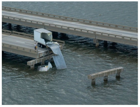
Figure 1.
A public-domain photo of a coastal bridge destroyed by Hurricane Ivan in Florida [12].
In recent years, in addition to numerical modeling, artificial intelligence (AI) has become a valuable approach in engineering applications [13,14]. Kufel et al. (2023) [15] and IBM (2016) [16] describe the relationship among artificial intelligence (AI), machine learning (ML), deep learning (DL), and neural network (NN) as a series of AI systems from largest to smallest, each encompassing the next, as shown in Figure 2. AI serves as the overall framework. ML is a subset of AI. Deep learning is a specialized area within ML. NN forms the foundation of deep learning algorithms. Dependent on the complexity of the study and amount of data, researchers may use shallow learning or deep learning in their machine learning studies. Shallow learning neural networks generally consist of only one hidden layer [17], making them faster to train and requiring less computational resources. By comparison, deep learning neural networks consist of many hidden layers [17,18] to achieve better accuracy for tasks with more complexity, which are more expensive and require more resources. One of the shortcomings in AI modeling is the limitation of data because most AI models are driven by data. Hybrid models that combine AI algorithms with traditional numerical methods have been developed in some studies that use data produced by numerical models.

Figure 2.
Schematic diagram to show relationship among AI, ML, DL, and NN. Shallow network consists of only one hidden layer.
Long Short-Term Memory (LSTM) is one of the deep learning neural networks that is popularly used in many different engineering fields. Li et al. (2022) [19] integrated LSTM with a convolutional neural network to simulate wave-induced loads for marine structures. Based on laboratory experimental data, Zhu et al. (2023) [20] applied the LSTM model to investigate wave–bridge interactions. Kar et al. (2024) [21] used LSTM to predict wave height in extreme events. Liu et al. (2023) [22] used LSTM in vessel trajectory prediction. Wang et al. (2023) [23] conducted LSTM simulation of wave propagation on the coast of Chesapeake Bay. Wu et al. (2024) [24] conducted 2D modeling of wave heights by using deep LSTM. In laboratory experiments, Zhang et al. (2024) [25] applied LSTM in real-time control and wave force predictions. Alizadeh and Nourani (2024) [26] applied LSTM networks in wave forecasting up to 6 h ahead with field buoy recorded data. Wang and Ying (2023) [27] presented integrated LSTM with GRU to predict ocean wave height based on field buoy data. Luo et al. (2022) [28] used Bi-LSTM model to simulate significant wave heights during hurricanes in the Atlantic Ocean. Yan et al. (2023) [29] conducted a study of time series prediction based on LSTM neural networks for the top tension responses of umbilical cables. Other LSTM model applications include Zheng (2019) [30], Xue et al. (2021) [31], and Chen et al. (2022) [32]. There are some other types of deep learning methods and systems. Lu et al. (2024) [33] applied a physically informed neural network (PINN) to investigate wave distribution. It solves the governing partial differential equations of physical phenomena using deep learning. Chen et al. (2023) [34] presented a study mapping coastal bathymetry by using PINN. Ahn and Kim (2021) [35] applied a neural network for extreme load prediction. Altunkaynak and Wang (2011) [36] used an expert system of Geno–Kalman Filtering (GKF) and fuzzy logic to predict the concentration of total suspended solids.
Feedforward neural network (FFNN) is among the most widely used types of neural networks, as described by Portillo and Negro (2022) [37] in their review of different types of AI applications in ocean engineering and other research fields [38,39,40,41,42]. A FFNN with one hidden layer is considered a shallow learning FFNN [18], while those with many hidden layers are deep learning networks. There are some successful references of applications of FFNNs in ocean engineering and oceanography [43,44,45,46,47,48]. Chen et al. (2024) [49] presented a decision-aid system for risk intervention based on a backpropagation neural network with a small dataset. Gao et al. (2024) [50] conducted a rapid prediction of an indoor airflow field using an operator neural network. Wu et al. (2020) [51] used the GAIFOA-BP neural network to predict strain under different loading of stored oil. Other FFNN applications include those detailed by Gabella (2021) [52], Li and Zhang (2021) [53], and Zhang and Liu (2023) [54]. In general, for modeling time series with neural network models, sequential data without gaps are used as inputs, and the model produces sequential data as outputs.
Because of FFNN’s advantage in recognizing patterns to correlate inputs and outputs, FFNNs with one hidden layer have been used in our previous studies for different applications, examples including modeling estuarine salinity in response to river flow and tides [55], tidal predictions in coastal inlets [56], storm surge predictions [57], tidal currents across coastal channel [58], long-term estuarine salinity variation in response to river flow and wind [59], and river flow predictions [60,61]. An FFNN with optimized backpropagation algorithms in model training and verification has been shown to be effective in our previous studies. Due to the straightforward manner in which feedforward neural networks can be configured, FFNNs have good advantages in pattern recognition to correlate between inputs and outputs when an optimized training algorithm is employed, which provides good reference for the wave load predictions in this study.
In recent years, the comparison of deep and shallow neural networks has sparked considerable research interest across various fields, with studies yielding diverse outcomes. For network security studies, Kim and Golfman (2018) [17] revealed that shallow neural networks were more accurate. In computer science studies, Herrera et al. (2022) [62] demonstrated that a deep neural network is better if the study situation has natural symmetries. Otherwise, shallow learning is expected to be more effective. Through the comparison of deep and shallow learning architectures, Meir et al. (2023) [63] found that the error of the shallow network decreased as a power law with the quantity of filters in the initial layer. This indicates that a shallow learning neural network can accomplish similar low errors as those from using more expensive deep learning architectures. However, no study has been performed comparing shallow and deep learning neural networks in coastal wave load studies.
In this study, we will evaluate and compare deep LSTM and shallow FFNNs in predicting hurricane wave loads on bridge decks. Data from previous full-scale numerical simulations of wave loads on bridges during two hurricanes will be used to train and verify the network performance of the deep LSTM and shallow FFNNs. The bridge deck broken by the Category 4 Hurricane Ivan in Florida is shown in Figure 1. This research seeks to deliver useful information for evaluating the effectiveness of deep and shallow learning neural networks for simulating extreme wave forces during hurricanes. The findings are expected to benefit ocean engineering design and coastal hazard mitigation efforts.
2. Description of Shallow FFNN and Deep LSTM Methodology
2.1. Shallow FFNN for Wave Load Modeling
A feedforward neural network (FFNN) is a fundamental type of neural network. Data flow forward from the input layer to the output layer, passing through one or more hidden layers. FFNNs do not have cycles or loops. Haykin (1999) [64] describes the basic theories and Li et al. (2022) [19] provide more recent overviews and descriptions of FFNNs. An FFNN can be trained to establish the correlation between inputs and target outputs. In an FFNN, outputs are linked to inputs via neurons that utilize weights and biases. An FFNN’s performance is determined by neuron connections in the network design and the magnitude of their weights and biases. The network repeatedly changes its weights and biases during training based on a specified algorithm. It continues until the anticipated error rate is achieved. FFNNs often use backpropagation optimization algorithms to train and improve their accuracy. Based on the method described in Haykin (1999) [64] and Li et al. (2022) [19], a shallow FFNN for wave loads designed for this study is shown in Figure 3. The FFNN includes three layers: one input layer, one hidden layer, and one output layer. Xi stands for the inputs; Yi means the neurons in the output layer. The input weights (Wij) are linked to the inputs. The output weights (Wjk) are linked to the output layer.
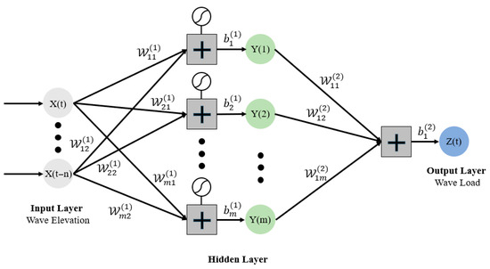
Figure 3.
Schematic diagram of the three-layer shallow learning FFNN model for wave loads proposed for this study. The FFNN consists of only one hidden layer.
The weights and biases in the FFNN have to be trained by data. The most common procedure is to divide the datasets into two parts: one for network training, and another for network verification [38]. Various training algorithms are available that produce different computation speeds in FFNN training and accuracy in network verifications. The most common one used in FFNN model training is the backpropagation (BP) algorithm [65,66]. The standard or basic backpropagation training method is the gradient descent method [65]. Optimized training methods can improve FFNN model training [38,64,66]. Huang and Murray (2008) [58]’s applications of FFNNs in tidal current simulations show that optimized SCG backpropagation [67] is efficient.
The major formula of the FFNN is given below:
where the elements of and denote the input and output weights, respectively. indicates the hidden layer activation function (tanh in this study), and represents the output activation function, which is linear for the regression task.
The Levenberg–Marquardt algorithm (LM) backpropagation (BP) training algorithm [64] is an optimized method that provides fast and accurate training. Therefore, the LM algorithm is one of the optimal options for fast and accurate training for our FFNN model. Rehman et al. (2024) [68] used Levenberg–Marquardt backpropagation to predict hydrodynamic forces for fluid over multiple cylinders. This provides a good reference for us to simulate hurricane wave forces. Considering that the LM algorithm has not been used in our previous investigations, it will be evaluated in this study and will be compared with other algorithms.
In this study, the three layers of the feedforward network (FFNN) are designed, as shown in Figure 4, to recognize the correlation and pattern between the wave elevation and wave loads. The hidden layer employs a hyperbolic tangent transfer function. The output layer adopts a linear transfer function. The network design and programming are conducted using the MATLAB Deep Learning Toolbox [69]. For the inputs of wave elevations, a sequential input of x = {X(t − i), …, X(t − 3), X(t − 2), X(t − 1), X(t)} is used to predict wave load outputs Z(t) at time t. The amount of data is selected based on a model sensitivity study.
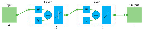
Figure 4.
Flow chart of shallow FFNN model with the number of neurons for wave loads with input of wave elevation.
To minimize overfitting problems, the number of neurons in the FFNN hidden layer was estimated by applying Fletcher and Goss (1993)’s approximation method [70]. The FFNN was trained by applying 50–60% of the data and then validated with the remaining 50–40% of the data. Through a series of initial tests, as discussed later in the model sensitivity study given in the discussion section later, the FFNN with 15 neurons in the hidden layer was selected as shown in Figure 4. Its size resulted in a low error and high correlation between inputs and outputs. The FFNN was trained and verified by using the data generated from our previous numerical wave load modeling studies [10,11]. The data covered two hurricane events: Hurricane Ivan which landed in Florida and Hurricane Katrina which landed near New Orleans. Input data included time series of hurricane wave elevations at the current time step and wave data in the past three consecutive time steps. Outputs from the FFNN were the time series of wave forces.
2.2. Deep LSTM Neural Network for Wave Load Modeling
A Long Short-Term Memory (LSTM) network is a specialized variant of a Recurrent Neural Network (RNN). It was described in detail by Hochreiter and Schmidhuber (1997) [71] and discussed further by MathWorks (2024) [69]. LSTMs are widely employed for tasks involving sequential data, with examples including learning, processing, and classification, due to LSTMs’ ability to capture and maintain long-term dependencies across time steps. Unlike standard RNNs, which often struggle with issues like the vanishing or exploding gradient during backpropagation, LSTM networks are designed with additional gates. These gates regulate the flow of information. They determine what is retained, discarded, or passed on to subsequent hidden states. Therefore, the gates enable the network to effectively capture long-term patterns. The reduced sensitivity to time gaps gives LSTM networks an advantage over traditional RNNs when handling sequential data. The architecture of an LSTM network includes an input layer, one or more hidden layers, and an output layer. The LSTM uses a memory block in the unit. As illustrated in Figure 5, this memory block includes three gate functions, each playing a distinct role in the information flow process. A sequential of inputs is x = {X(t − i), …, X(t − 3), X(t − 2), X(t − 1), X(t)}. The output sequence outputs are h = {h1, h2, h3, …, hi}. The forget gate is a critical component. It determines whether the current information should be forgotten or retained.
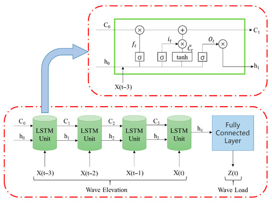
Figure 5.
Schematic diagram of LSTM architecture with 15 hidden units for wave load modeling. Major equations of LSTM are given below.
Mathematically, at a specific time step t, the formulas can be expressed as follows:
where and are the forget weight matrix and the forget hidden weight matrix, respectively; is the bias of the forget gate; and is the sigmoid function.
The input gate determines the information updating, and memorizes the new information. They are defined as follows:
where and denote the weights of the matrices associated with the input gate, and and are the weight matrices associated with the candidate memory cell. and are the bias vectors of the input gate and the updating cell state, respectively. Then, the new memory cell state is updated as follows:
where is the previous memory cell state and represents the element-wise product.
Finally, the output gate controls the output activations, and the hidden state sent to the next time step is defined as follows:
where is the output hidden weight matrix, represents the output weight matrix, and is the bias of the output gate.
In this study, we employ an LSTM network with the following architecture and parameters: In the input layer, input data include the time series of hurricane wave elevations at the current time step and wave data in the past three consecutive time steps. In the output layer, the time series of wave forces are output from the LSTM. The LSTM’s hidden layer consists of 15 hidden units based on the sensitivity study of different number of neurons. A regression layer is employed for calculating the loss for regression tasks.
2.3. General Neural Network Training and Verification Process
Two different datasets are prepared: one for model training and another for model validation. For network training, a model’s maximum iteration number and error are specified. During model training, the model performs simulations to reduce the errors between model-simulated best value and target goal (or actual value). If the error has not reached the goal, the network continues to adjust the networks’ parameters (weights and biases) until either the error reaches the given allowance value or reaches the defined maximum number of iterations. During verification, the trained neural network no longer adjusts its weights and biases. Instead, it directly uses the trained weights and biases to calculate the output values based on the given inputs without any iteration. Therefore, the correlation values during verification are used to evaluate if the network is good or overfitting. The network structure with the best correlation coefficient and minimum error will be selected for the application.
3. Case Study I: Simulation of Wave Loads During Hurricane Katrina for Submerged Bridge Deck in Biloxi Bay
3.1. Data Obtained from Full-Scale Numerical Wave Model Simulations of Biloxi Bay Bridge
Data for neural network studies are obtained from our previous CFD wave dynamic modeling studies. The dynamic wave load model employed in the present study has been satisfactorily validated in several earlier studies by comparing simulation results with laboratory experimental data or analytical solutions (e.g., Xiao and Huang, 2008, 2010, 2015, 2024 [72,73,74,75]; Huang and Xiao, 2009 [10]; Xiao et al., 2010, 2009, 2013 [11,76,77]. For example, Xiao and Huang (2008) [72] simulated solitary wave runup and forces on a vertical wall and compared the results with the analytical solutions of Fenton and Rienecker (1982) [78]. The time history of wave forces on the wall showed an overall correlation coefficient of 0.997 and an RMSE of 0.001. In addition, when compared to the laboratory data on uplift forces acting on coastal bridge decks from French (1969) [79], numerical results by Huang and Xiao (2009) [10] yielded a high correlation coefficient of 0.981 and a low RMSE of 0.0809. This provides strong quantitative evidence that the wave load model performs excellently in computing wave-induced forces on coastal bridge decks. More recently, in a comparison with three-dimensional experiments by Park et al. (2018) [80] on wave runup and slapping forces on an elevated house, the simulations by Xiao and Huang (2024) [75] achieved a correlation coefficient of 0.932 and an RMSE of 0.078, demonstrating the model’s capability in simulating 3D wave forces.
In 2005, Hurricane Katrina passed by Biloxi Bay in Louisiana. A significant portion of the bridge deck was impaired by waves and storm surges. Xiao et al. (2010) [11] conducted numerical wave load modeling. The study simulated wave forces for the submerged deck condition, as shown in Figure 6a. Initial surge water elevation was at the surface of the deck (Figure 6a). The numerical model was satisfactorily validated by comparison with experimental data before its application to the hurricane case study. Model simulations characterized wave–structure interactions, as shown in Figure 6b. The results revealed that the maximum force was greater than the deck weight. This caused the failure of the deck.
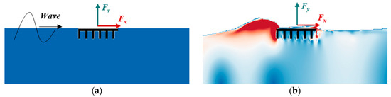
Figure 6.
Submerged bridge of horizontal force Fx and vertical force Fy during Hurricane Katrina: (a) initial water elevation, (b) example of wave–structure interaction.
The wave elevation and forces from Xiao et al.’s (2010) [11] study are used as data in this study to train and verify our shallow FFNN model and deep LSTM network. The storm surge elevation is 8.57 m at the top of the bridge deck, wave height is 2.60 m, and wave period is 5.5 s. Data are in 0.5 s intervals across approximately 10 wave periods. Therefore, there are about 12 data points in a wave period. Based on a model sensitivity study, the inputs of wave elevation data covering about 1/3 of the wave period, x = {X(t − 3), X(t − 2), X(t − 1), X(t)}, are used to provide good training and verification of the wave loads at the time Z(t). The data from the first six periods are employed for training the shallow FFNN and deep LSTM networks, while the remaining four periods are used for verification.
3.2. Shallow FFNN Training and Verification for Wave Loads for Hurricane Katrina
The shallow FFNN with one hidden layer, as shown in Figure 3 and Figure 4, was used to simulate wave forces. The hidden layer had 15 neurons. Ten different backpropagation algorithms were examined (Table 1) and the optimized Levenberg–Marquardt backpropagation algorithm was selected. We established a maximum of 200 epochs for the FFNN model training. In order to compare with the LSTM method, we used a very small truncational error (1.0 × 10⁻⁸) so that the model training was controlled by the maximum epochs. As shown in Figure 7, the best training performance of horizontal force reduced the mean square error to 1.654 × 10⁻⁶ with a correlation coefficient of 0.999 after the training stopped at 200 epochs; for the vertical wave force, the training performance showed a mean square error of 9.919 × 10⁻⁷ with a correlation coefficient of 0.999. In general, the training performance was very good when using the Levenberg–Marquardt backpropagation algorithm.

Table 1.
Hurricane Katrina case study: comparison of performance of different training algorithms for modeling of horizontal wave force.
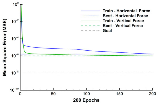
Figure 7.
Shallow FFNN training using LM training algorithm for wave forces during Hurricane Katrina.
After achieving the maximum training epochs, the FFNN is verified by using the remaining data. Using the inputs of wave elevation (Figure 8a), the FFNN predictions of horizontal force closely align with the data from the numerical model (Figure 8b), demonstrating a 0.999 correlation coefficient. Deviations between the FFNN predictions and the actual data primarily occur near the peak force, where the horizontal force rapidly transitions from increasing to decreasing. In contrast, a simple linear regression between the wave elevation and horizontal force yields a much lower correlation coefficient of 0.61. The FFNN model predictions of vertical forces also closely match the data from numerical wave load modeling (Figure 8c), achieving a 0.999 correlation coefficient. The maximum deviations are observed near the regions of minimal wave force, where fluctuations are likely due to turbulence from wave breaking and wave–structure interactions. Comparatively, simple linear regression between the wave elevation and vertical force results in a very poor correlation, with a coefficient of 0.47. These results show that our multilayer FFNN model, optimized with the LM training algorithm, is able to correlate the nonlinear relationships between wave elevation inputs and the complex wave load outputs, similar to those derived from sophisticated but time-consuming CFD numerical wave models.
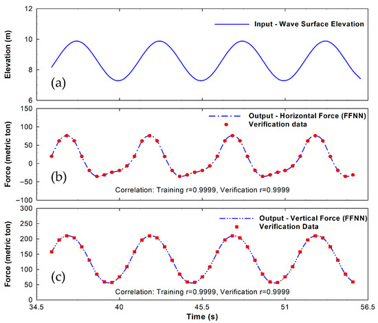
Figure 8.
FFNN verification for horizontal and vertical wave forces during Hurricane Katrina using LM training algorithm.
3.3. Deep LSTM Training and Verification for Wave Loads During Hurricane Katrina
Based on the deep LSTM network, as shown in Figure 5, the LSTM was trained by the adaptive moment estimation (Adam) optimization training method. We established the same number of maximum epochs of 200 as that for the FFNN model training so that we could compare the LSTM and FFNN model performance under the same epochs, as shown in Figure 9. For the dataset of ten wave periods, we used the first six wave periods of data for deep LSTM network training, and the remaining four wave periods of data for network verification. Model inputs consisted of wave elevations (Figure 10a). The outputs consisted of horizontal and vertical forces (Figure 10b,c).
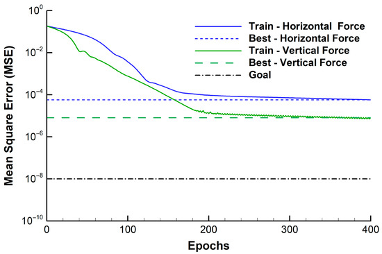
Figure 9.
Deep LSTM training using Adam optimizer for Hurricane Katrina.
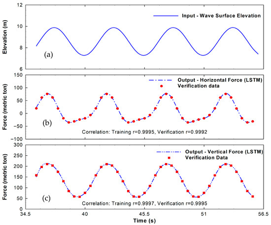
Figure 10.
Deep LSTM verification for horizontal and vertical wave force during Hurricane Katrina using Adam training optimizer.
After 200 epochs of network training, the correlation coefficients between model and data reach 0.9995 for horizontal force. The correlation coefficient for vertical force is 0.9997. After the satisfactory training, the trained LSTM network is validated by the remaining four periods of wave and force data for model verification. As shown in Figure 10, deep LSTM network simulations of wave forces align closely with the data. Despite the time series of horizontal force showing the nonlinear feature, the deep LSTM predictions reproduce the nonlinear pattern. For the verification data, the LSTM network produces the correlation coefficient of 0.9992 for horizontal force and 0.9995 for vertical force. The RMSE is 0.0171 for horizontal force and 0.0076 for vertical force, respectively.
3.4. Comparison of FFNN and LSTM for Hurricane Katrina Case Study
Statistics of shallow FFNN and deep LSTM model performance for horizontal wave forces are given in Table 1. It shows that both FFNN and LSTM are affected by the usage of different training algorithms. Therefore, selecting an appropriate training algorithm is important to achieve the desired accuracy for both deep LSTM and shallow FFNNs. For deep LSTM networks, three training algorithms have been investigated. Among them, adaptive moment estimation (Adam) results in the best result with the optimal correlation of 0.9992 and the minimum RMSE of 0.0171. By comparison, the best result from the shallow FFNN method is produced by the Levenberg–Marquardt algorithm (LM) backpropagation (BP) algorithm (Trainlm). It achieves a minimum RMSE error of 0.0014 with an optimal correlation coefficient of 0.9999. The shallow FFNN-LM method produces an equivalent correlation coefficient but with a lower RMSE by comparing with the LSTM using the adaptive moment estimation training optimizer. In addition, the training time for LSTM-LM is approximately four times faster than that for the LSTM (Table 1).
For deep LSTM networks, we have investigated three training methods: (a) stochastic gradient descent with a momentum (Sgdm) optimizer; (b) a root mean square propagation (Rmsprop) optimizer, which is a stochastic solver; (c) an adaptive moment estimation (Adam) optimizer for more efficient stochastic optimization to make the LSTM model perform even better. As shown in Table 1, all three training methods produce very high correlation coefficients above 0.985 for the verification dataset. The adaptive moment estimation (Adam) optimizer results in the highest correlation of 0.9992 with the minimum root mean square error of 0.0171 among the three training methods.
Referring to MatLab (Version 2023) [69], the training algorithms shown in Table 1 are described below. Sgdm is stochastic gradient descent with momentum. Rmsprop is root mean square propagation. Adam is adaptive moment estimation optimizer. Traingd is gradient descent backpropagation. Traindgx is gradient descent with momentum and adaptive learning rate backpropagation. Trainscg is scaled conjugate gradient backpropagation. Trainlm is Levenberg–Marquardt backpropagation. Trainrp is resilient backpropagation. Traingdm is gradient descent with momentum backpropagation. Traincgf is conjugate gradient backpropagation with Fletcher–Reeves updates. Traincgb is conjugate gradient backpropagation with Powell–Beale restarts. Trainbfg is BFGS quasi-Newton backpropagation. Traincgp is conjugate gradient backpropagation with Polak–Ribiére updates.
For a shallow FFNN, ten training algorithms available in MATLAB (Version 2023) have been evaluated. Results indicate that all training algorithms result in good results with correlation coefficients above 0.9235. Among all FFNN training algorithms, the basic gradient descent (Traingd) training algorithm takes the shortest time in model training and results in the largest error of 0.1888 with the lowest correlation coefficient of 0.9235. By comparison with the deep LSTM-Adam results of a correlation coefficient of 0.9992 and RMSE of 0.0171, as shown in Table 1, seven out of ten shallow FFNN training algorithms (Trainscg, Trainlm, Trainrp, Traincgf, Traincgb, Trainbfg, Traincgp) produce higher correlation coefficients and lower RMSE. In addition, the shallow FFNN’s training time is approximately 4 times faster than LSTM’s training time.
4. Case Study II: Simulation of Wave Loads During Hurricane Ivan for Emerged Bridge Deck in Escambia Bay
4.1. Data Obtained from Full-Scale Numerical Wave Model Simulations of Escambia Bay Bridge
A bridge near Pensacola in Florida was impaired by wave loads in Hurricane Ivan in 2004 (Figure 1). Huang and Xiao (2009) [10] conducted a numerical CFD modeling of wave force based on input of boundary wave elevation. The numerical model was validated by comparing simulations with data. The numerical model was then used to investigate wave forces during Hurricane Ivan (Figure 11). Initial water elevation was at the bottom of the structure (Figure 11a). An example of wave–structure interaction is shown in Figure 11b. Compared to the submerged condition, as shown in Figure 6b, the wave surface for the emerged structure in Figure 11b shows wave breaks in the wave–structure interactions. As a result, the wave forces (Figure 12b,c) show sharp nonlinear variations in comparison to the submerged structure case (Figure 8b,c). The sharp variations in wave force present a more complicated issue to test the LSTM and FFNN’s capability.
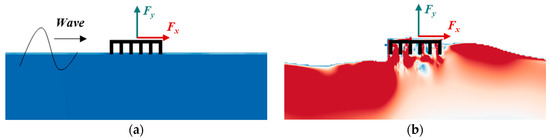
Figure 11.
Emerged bridge of horizontal force Fx and vertical force Fy in Hurricane Ivan: (a) initial condition; (b) example of wave–structure interactions and breaking.
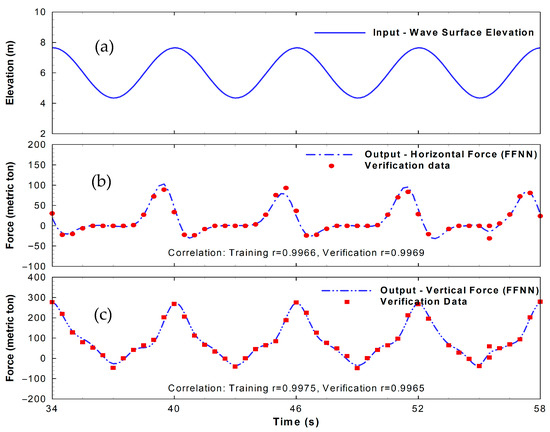
Figure 12.
FFNN verification for horizontal and vertical forces on the emerged bridge using the Levenberg–Marquardt BP algorithm.
The datasets from the CFD numerical modeling are used to investigate the FFNN and LSTM model performances. The dataset consists of wave elevations as inputs (Figure 12a). Horizontal and vertical wave forces serve as targets or outputs. Based on Huang and Xiao (2009) [10], the peak storm surge elevation is 6.0 m. The wave at the ocean boundary is about 150 m away from the bridge with a wave period of 6 s and a 1% highest wave height of 3.3 m. The time series of data are in 0.5 s intervals for 10 wave periods. Therefore, there are about 12 data points in a wave period. Based on a model sensitivity study, the inputs of wave elevation data covering about 1/3 of the wave period, x = {X(t − 3), X(t − 2), X(t − 1), X(t)}, are used to provide good training and verification of one output at time Z(t). Data for the first six wave periods are used for network training. Data for the remaining four wave periods are used as network verification. An example of wave action on the structure is given in Figure 11b. Comparing to the submerged deck condition as shown in Figure 6b, the emerged condition in Figure 11b shows wave breaking under the deck with a less smooth surface. Because of the wave breaking and wave–structure interactions due to the emerged structure’s condition (Figure 11b), the response of the wave forces (Figure 12b,c) is substantially different from the input of the wave elevation profile. Therefore, this case study can be used to evaluate the capability of deep LSTM and shallow FFNNs in predicting highly nonlinear wave forces on bridges.
4.2. Shallow FFNN Training and Verification for Hurricane Ivan
The shallow FFNN with only one hidden layer (Figure 3 and Figure 4) was applied to simulate wave forces. Fifteen neurons were used in the hidden layer. Ten different backpropagation algorithms were examined (Table 2) and the optimized Levenberg–Marquardt backpropagation algorithm was selected for presentation here. We established a maximum of 200 epochs for the FFNN model training for the purpose of comparison with the deep LSTM method. Levenberg–Marquardt BP was selected after the evaluation of ten different training algorithms, as shown in Table 2. Based on the inputs from boundary waves located approximately 150 m from the bridge site, data from previous numerical wave load modeling were applied to FFNN training and verification. The first six periods of data were allocated for training the FFNN model, while the subsequent four periods were used for verification.
Table 2.
Hurricane Ivan case study: comparison of different training methods for modeling horizontal wave force by LSTM and FFNNs.
The satisfactorily trained FFNNs are verified using the remaining data. The horizontal force displays a pattern significantly different from the wave elevation (Figure 12), showing strong nonlinearity. For horizontal force, while simple linear regression between the boundary wave elevation and wave force results in a very low correlation coefficient of 0.36, the shallow FFNN predictions of horizontal force align closely with the data, achieving a 0.9969 correlation and very low 0.0227 RMSE. For the vertical wave force in Figure 12, the FFNN model recognizes the historical pattern and satisfactorily predicts vertical wave force with a very high correlation coefficient of 0.9965, which is much better than the simple linear regression between the boundary wave elevation and wave force for a very low correlation coefficient of 0.47. Even the sharp changes in the peak wave forces match well between the data and the shallow FFNN model predictions, indicating that FFNN with the Levenberg–Marquardt backpropagation algorithm is capable of providing accurate predictions of nonlinear wave forces on bridges. Three training algorithms have been tested, including Sgdm, Rmsprop, and Adam.
4.3. Deep LSTM Training and Verification for Wave Forces During Hurricane Ivan
For the Hurricane Ivan case study, the deep LSTM model as shown in Figure 5 has been adopted to simulate wave forces. The LSTM model consists of 15 hidden units. Time series of wave elevation are used as input. The maximum simulation epoch is 200 which is the same as those specified for FFNN model simulations for model comparison. The first six wave periods of data are used for model training, while the remaining four wave periods of data are used for model verification. Three training algorithms have been tested, including Sgdm, Rmsprop, and Adam. Although LSTM networks with all three training algorithms produce satisfactory results as shown in Table 2, the Adam training optimizer results in the best results with the strongest correlation coefficient and the lowest error.
After the LSTM-Adam network has been satisfactorily trained, it is applied to predict the wave forces by the remaining data for verification. As shown in Figure 13, corresponding to the time series of wave elevation as input, LSTM model predictions of wave forces align closely with the overall trend of the data. The correlation coefficients are 0.9858 for the horizontal force and 0.9924 for the vertical force, respectively. For horizontal force, as shown in Figure 13, the LSTM slightly underestimates some peak wave force values. For vertical wave force, all peaks of vertical wave forces match well between LSTM predictions and data.
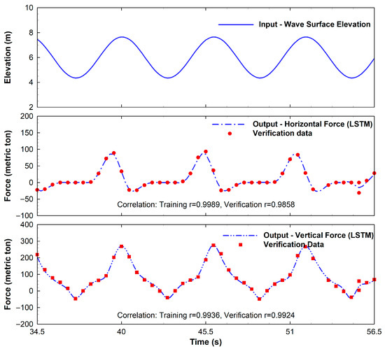
Figure 13.
Deep LSTM network verification for horizonal and vertical forces on the emerged bridge using Adam training optimizer.
4.4. Comparison of Shallow FFNN and Deep LSTM for Hurricane Ivan
A comparison of horizontal force verifications resulting from the shallow FFNN and deep LSTM networks is shown in Table 2. The LSTM network with the Adam training optimizer produces a very good correlation of 0.9858 and RMSE of 0.0439, which are comparatively better than the other two training algorithms (Sgdm and Rmsprop). Compared to LSTM-Adam’s correlation coefficient and RMSE, FFNN with eight out of ten backpropagation algorithms is shown to produce an equivalent or better correlation coefficient (above 0.9858) and lower RMSE (below 0.0439). In addition, the FFNN training times for different training algorithms are faster than LSTM’s training time by 3–5 times. But model verification in FFNN takes 2 times as much time as LSTM. The FFNN with the Levenberg–Marquardt BP algorithm results in 0.9969 correlation and 0.0227 RMSE, showing higher accuracy than the results obtained by LSTM-Adam.
5. Discussion
5.1. Data Gaps and Noise
The time series modeling by neural networks requires continuous data inputs. For the inputs of wave elevations, a sequential input of x = {X(t − i), …, X(t − 3), X(t − 2), X(t − 1), X(t)} is used to predict wave load Z(t) at time t. Therefore, users are unable to randomly select time series of data with data gaps in model training and verification. If data gaps exist in the input dataset, data processing has to be conducted to fill the data gaps before the data can be used by the neural network model.
If field measurement data with noise and gaps are available for neural network modeling, data processing and analysis have to be conducted first. Low-pass filters can be used to remove noise signals. For coastal waves, spectrum and frequency analysis may be used to identify the dominant wave frequencies or periods. Then, data gaps can be approximately filled by extending the dominant periodic wave signals. Huang and Xu (2009) [57] presented a good example of integrating low-pass filter and harmonic analysis to recover missing storm surge data during hurricanes in Florida.
5.2. Neural Network Versus Numerical Wave Load Model
After training, neural networks produce weight files that enable rapid and efficient wave load predictions. Consequently, both the FFNN and LSTM models can forecast wave force time series in under 0.09 s (as shown in Table 1 and Table 2) in model verification. The training durations for the two neural networks are relatively short, with maximum times recorded at 1.2269 s for the FFNN and 3.7123 s for the LSTM (Table 1 and Table 2, respectively). In contrast, the computational time consumed by the numerical wave load model is much longer. For instance, modeling 10 wave cycles takes around 33 min for the Hurricane Ivan case and approximately 38 min for the Hurricane Katrina case on the current computer system (Intel Core i5-8400, 2.80 GHz). In other words, neural network simulations are over 600 times faster than CFD wave load modeling in terms of computation speed.
When data, either from observation or CFD modeling, are available for training and verifying the model, both the FFNN and LSTM models in this study demonstrate their capability for rapid computation and deliver satisfactory predictions of hurricane wave load on coastal bridges. Therefore, we can use field observed data to perform quick predictions of wave loads on bridges. In addition, considering that traditional numerical CFD wave load modeling is time-consuming and costly, a hybrid modeling approach that integrates numerical wave load modeling with the FFNN or LSTM networks may be employed in future research. Traditional numerical CFD wave load models can be used to simulate wave loads and storm surges to generate a comprehensive dataset for wave loads under hurricane or extreme weather conditions. This large dataset would then be used to train the FFNN and LSTM models to provide cost-effective and rapid predictions of hurricane wave loads under various scenarios. Despite the fast simulation speed, neural networks have some limitations in comparison to CFD modeling. CFD models are physical-based models that can be used to investigate more details of the physics of the fluid, flow velocity fields, vortices, flow pressure, and wind forces.
The neural network models can also be used as supplemental tools to support expensive lab or field measurements of wave loads by using limited data to train the model for investigating more scenarios of wave loads under different wave conditions.
5.3. Shallow FFNN vs. Deep LSTM Neural Networks
The question of whether deep learning outperforms shallow learning has attracted research interest and discussion in recent years [18,61,62]. In some cases, deep learning is better than shallow learning [61]. In other cases, shallow learning is better than deep learning [18]. Our results present a comparison between deep learning and shallow learning for wave load studies in coastal and ocean engineering. Based on the two case studies of hurricane events (Table 1 and Table 2), both shallow FFNN and deep LSTM are shown to be capable of providing satisfactory predictions of time series of dynamic wave loads on bridges by using the inputs of wave elevations. For both FFNN and LSTM, the selection of appropriate training algorithms is important to achieve the neural network prediction accuracy. Different training methods may result in different accuracies and computation times. The shallow FFNN-LM network is one of the best training methods for FFNNs. The LSTM-Adam is the most accurate training optimizer for LSTM networks. In our two case studies, the FFNN-LM network demonstrates faster performance and slightly higher accuracy than the LSTM-Adam network. Levenberg–Marquardt (LM) optimized backpropagation is highly effective for training small-to-medium-sized neural networks because it combines the fast, second-order convergence of the Gauss–Newton method with the stability and robustness of the first-order gradient descent method. LM provides superior optimization for appropriate network types and datasets, but may be memory-intensive for large-scale deep learning. For our case study, the dataset is relatively small, which makes Levenberg–Marquardt (LM) optimized backpropagation effective. Deep learning LSTM has been recognized for its advantage in time series forecasting for large datasets. In this study, it has shown a very good correlation coefficient above 0.98. However, because our dataset is small, both FFNN and LSTM perform well, but FFNN has a slight advantage for small dataset problems. For networks with large datasets, LSTM may have some advantages.
There are other machine learning methods that may be worthy of investigation in the future. For example, Gated Recurrent Units (GRUs) are a type of Recurrent Neural Network (RNN) that address the challenges of traditional RNNs in learning long-term dependencies, using reset and update gates to control information flow and maintain relevant context in sequential data. GRUs are computationally efficient, have fewer parameters than LSTMs, and are effective for time series prediction where moderate sequential dependencies are present.
5.4. Effect of Network Size
In neural network models, increasing the number of neurons or units typically raises computational complexity. However, this increase does not always lead to better performance, particularly when the training dataset is small, as it can cause overfitting and reduced prediction accuracy. Consequently, selecting approximate neuron numbers is crucial to the improvement of the model’s generalization ability. This section uses the case of Hurricane Ivan to demonstrate the effects of network size. Different neuron/unit configurations (e.g., 5, 10, 15, 20, and 30) are applied to both FFNN and LSTM models, and horizontal force predictions are generated for each configuration. Table 3 shows that variations in the number of neurons/units significantly influence the correlation coefficient and RMSE error of horizontal force predictions for both FFNN and LSTM models, underscoring the critical role of neuron count in determining model performance.
Table 3.
Comparison of performance between shallow FFNN-LM and deep LSTM-Adam models with varying neuron sizes or units in the hidden layer for predicting the time history of horizontal forces during Hurricane Ivan.
In the FFNN-LM model, training and validation times exhibit minimal fluctuation, but prediction accuracy improves considerably as the number of neurons increases, peaking at 15 neurons with a 0.9969 correlation and an RMSE of 0.0227. However, as the number of neurons increases to 20 and 30, the model shows signs of overfitting, leading to a decline in accuracy. This trend suggests that using too few neurons results in underfitting, limiting the model’s capacity to capture essential data features. However, an excessive number of neurons leads to overfitting, thereby reducing the model’s generalization ability.
In contrast, the LSTM-Adam model demonstrates a gradual increase in training time as the number of hidden units rises, although its correlation coefficient and RMSE show small variations. The model achieves its best performance with 10 hidden units, yielding a 0.9902 correlation and RMSE of 0.0383. Beyond this point, both metrics remain relatively stable despite increases in hidden units. This behavior could be due to the LSTM’s inherent complexity, which may limit the benefits of adding more hidden units, especially with a relatively small dataset. Moreover, the LSTM model is more computationally intensive, with training time increasing substantially as hidden units are added, reflecting the higher resource demands of recurrent architectures in handling sequential data.
5.5. Spatial and Temporal Neural Network Modeling
In future studies, the time series modeling of neural networks may be expanded to investigate both spatial and temporal variations in wave pressure fields and forces acting on coastal structures. Wang et al. (2025) [81] provide a good reference for applying the neural network framework for high-resolution velocity fields in wave–structure interactions to provide more details of wave actions on coastal bridges during hurricanes. The spatial and temporal modeling by artificial neural networks may also be used to provide rapid predictions of storm surges to support real-time hurricane evacuations in Florida and the coast of the Gulf of Mexico. Traditional hydrodynamic modeling of hurricane-induced storm surges and waves (e.g., Huang et al., 2022 [82]; Vijayan et al., 2021 [83], 2023a [84], 2023b [85]; Ullman et al., 2019 [86]; Ma et al., 2024a [87], 2024b [88]) is time-consuming even using high-performance computers. Hurricane evacuations often require fast updates of both spatial and temporal distributions of storm surge and wave predictions when uncertainty of hurricane tracks are updated as hurricanes approach the coast (Alisan et al., 2020 [89]; Ghorbanzadeh et al., 2021 [90]; Yang et al., 2023a [91], 2023b [92], 2025 [93]). While neural networks have been used in some applications for coastal storm surge and wave modeling (e.g., Chondros et al., 2021 [94]; Wei et al., 2022 [95]; Qin et al., 2023 [96]; Ma et al., 2025 [97]), they require big data for network training and verification. Coastal and ocean hydrodynamic modeling may provide necessary data for spatial and temporal neural network training and verification. The trained and verified neural networks will then be able to provide rapid updates and predictions of storm surges and waves during hurricane events.
5.6. Limitation of Bridge Geometry
The scope of this study is to evaluate shallow learning and deep learning neural network models for hurricane wave force predictions. However, due to the limitations of wave and bridge geometry data, the case studies presented in this study are limited to only two selected bridge geometries. In future studies, if more hurricanes (including Ivan and Katrina) and more bridge geometries (including both bridges in Florida and Louisiana) are available, a generalized ANN model may be trained and verified by more broad big datasets for application to different hurricane events for different bridges.
6. Conclusions
Rapid and accurate predictions of hurricane wave forces on coastal bridges are important for assessing the causes of hurricane damage, supporting coastal structure design, and enhancing coastal resilience. Traditional numerical CFD modeling of hurricane wave loads, while comprehensive, is time-consuming and costly. Artificial neural networks provide a faster modeling approach for predicting wave forces. Whether deep learning or shallow learning neural networks are more efficient is dependent on different applications. For wave loads, the deep learning LSTM and shallow learning FFNN neural networks have been evaluated and compared in our investigations. Two case studies include an emerged bridge damaged by Hurricane Ivan in 2004 and a submerged bridge destroyed by Hurricane Katrina in 2005. Datasets were obtained from previous numerical wave load modeling studies for Hurricanes Ivan and Katrina. The deep LSTM network employs fifteen hidden units. The shallow FFNN has one hidden layer of fifteen neurons. The neural networks have been trained by the training dataset with the inputs of wave elevations and the targets of wave loads. Then, the trained neural networks are evaluated by another dataset for model verification.
To explore whether complex deep learning models outperform simpler shallow learning models for wave load predictions, the performances of deep LSTM and shallow FFNN have been evaluated and compared. Results indicate that both deep LSTM and shallow FFNN are able to provide very good accuracy in predictions of wave forces with correlation coefficients above 0.98 by comparing model simulations and data. Both LSTM and FFNN models’ performances are affected by the choice of training algorithms. The effects of different training algorithms, three for LSTM and ten for FFNN, were investigated. Results show that the best deep LSTM performance is achieved by the adaptive moment estimation (Adam) training optimizer. For shallow learning, FFNN-LM is among the most effective training methods for FFNNs. In general, shallow FFNN-LM network results in slightly better correlation coefficients and less error than those from the LSTM-Adam network for the wave force simulations. For the sharp variations in strongly nonlinear wave forces in the Hurricane Ivan case study of an emerged bridge condition, the FFNN-LM predictions of wave forces with a 0.997 correlation coefficient show better matches with the quick variations in peak wave forces than those from LSTM-Adam. The shallow FFNN-LM’s speed is approximately four times faster in model training but is about twice as slow in model verification or applications than those from the deep LSTM-Adam network, with a 0.986 correlation coefficient. The FFNN model is also almost 600 times faster than our previous numerical CFD wave modeling of wave loads in the case studies of Hurricanes Ivan and Katrina. However, the limitation of neural network models is contingent upon the availability of data. A hybrid modeling approach that integrates physical-based numerical wave load modeling and neural networks can be a good choice for wave load studies in the future.
Author Contributions
Conceptualization, H.X. and W.H.; methodology, H.X., W.H., and J.W.; validation, H.X. and J.W.; formal analysis, W.H.; investigation, H.X.; data curation, J.W.; writing—original draft preparation, H.X. and W.H.; writing—review and editing, W.H.; visualization, H.X.; supervision, W.H.; project administration, H.X.; funding acquisition, H.X. All authors have read and agreed to the published version of the manuscript.
Funding
This research was partially funded by the National Natural Science Foundation of China (Grant No. U22A20601) to support Hong Xiao’s time in preparing this manuscript.
Data Availability Statement
The raw data supporting the conclusions of this article will be made available by the authors on request.
Conflicts of Interest
The authors declare no conflicts of interest.
References
- Cruz, A.M.; Krausmann, E. Damage to Offshore Oil and Gas Facilities Following Hurricanes Katrina and Rita: An Overview. J. Loss Prev. Process Ind. 2008, 21, 620–626. [Google Scholar] [CrossRef]
- BOEM (Bureau of Ocean Energy Management). Newsroom Release #3486. Date: May 1, 2006. MMS Updates Hurricanes Katrina and Rita Damage. Available online: https://www.boem.gov/sites/default/files/boem-newsroom/Press-Releases/2006/press0501.pdf (accessed on 26 October 2025).
- Okeil, A.M.; Cai, C.S. Survey of Short- and Medium-Span Bridge Damage Induced by Hurricane Katrina. J. Bridge Eng. 2008, 13, 377–387. [Google Scholar] [CrossRef]
- Fan, X.; Zhang, J.; Liu, H. Numerical Analysis on the Secondary Load Cycle on a Vertical Cylinder in Steep Regular Waves. Ocean Eng. 2018, 168, 133–139. [Google Scholar] [CrossRef]
- Xie, P.; Chu, V.H. The Forces of Tsunami Waves on a Vertical Wall and on a Structure of Finite Width. Coast. Eng. 2019, 149, 65–80. [Google Scholar] [CrossRef]
- Xie, P.W.; Chu, V.H. The Impact of Tsunami Wave Force on Elevated Coastal Structures. Coast. Eng. 2020, 162, 103777. [Google Scholar] [CrossRef]
- Miao, Y.; Wang, K.H. Interaction between a Solitary Wave and a Fixed Partially Submerged Body with Two Extended Porous Walls. J. Eng. Mech. 2021, 147, 04021038. [Google Scholar] [CrossRef]
- Chen, M.; Huang, B.; Yang, Z.; Liao, L.; Zhou, J.; Ren, Q.; Zhu, B. Study on the Mechanical Characteristics and Failure Mechanism of the Coastal Bridge with a Box-Girder Superstructure under the Action of Breaking Solitary Waves. Ocean Eng. 2023, 287, 115834. [Google Scholar] [CrossRef]
- Yang, Z.; Zhu, B.; Huang, B.; Hou, J.; Zhang, Y.; Li, L. Numerical Study on the Behaviors of Coastal Bridges with Box Girder under the Action of Extreme Waves. Ocean Eng. 2023, 286, 115683. [Google Scholar] [CrossRef]
- Huang, W.; Xiao, H. Numerical Modeling of Dynamic Wave Force Acting on Escambia Bay Bridge Deck during Hurricane Ivan. J. Waterw. Port Coast. Ocean Eng. 2009, 135, 164–175. [Google Scholar] [CrossRef]
- Xiao, H.; Huang, W.; Chen, Q. Effects of Submersion Depth on Wave Uplift Force Acting on Biloxi Bay Bridge Decks during Hurricane Katrina. Comput. Fluids 2010, 39, 1390–1400. [Google Scholar] [CrossRef]
- NorthEscambia.com News. Available online: https://www.northescambia.com/2024/09/20-years-later-ivan-the-terrible (accessed on 19 October 2025).
- Floriano, B.; Hanson, B.; Bewley, T.; Ishihara, J.Y.; Ferreira, H.C. A Novel Policy for Coordinating a Hurricane Monitoring System Using a Swarm of Buoyancy-Controlled Balloons Trading off Communication and Coverage. Eng. Appl. Artif. Intell. 2025, 139, 109495. [Google Scholar] [CrossRef]
- Fatima, K.; Shareef, H.; Costa, F.B.; Bajwa, A.A.; Wong, L.A. Machine Learning for Power Outage Prediction during Hurricanes: An Extensive Review. Eng. Appl. Artif. Intell. 2024, 133, 108056. [Google Scholar] [CrossRef]
- Kufel, J.; Bargiel-Laczek, K.; Kocot, S.; Kozlik, M.; Bartnikowska, W.; Janik, M.; Czogalik, Ł.; Dudek, P.; Magiera, M.; Lis, A.; et al. What Is Machine Learning, Artificial Neural Networks and Deep Learning? Examples of Practical Applications in Medicine. Diagnostics 2023, 13, 2582. [Google Scholar] [CrossRef] [PubMed]
- IBM. IBM Data and AI Team. 2016. Available online: https://www.ibm.com/blog/ai-vs-machine-learning-vs-deep-learning-vs-neural-networks (accessed on 30 September 2024).
- Kim, D.E.; Gofman, M. Comparison of Shallow and Deep Neural Networks for Network Intrusion Detection. In Proceedings of the 2018 IEEE 8th Annual Computing and Communication Workshop and Conference (CCWC), Las Vegas, NV, USA, 8–10 January 2018; pp. 204–208. [Google Scholar]
- Emmert-Streib, F.; Yang, Z.; Feng, H.; Tripathi, S.; Dehmer, M. An Introductory Review of Deep Learning for Prediction Models with Big Data. Front. Artif. Intell. 2020, 3, 4. [Google Scholar] [CrossRef] [PubMed]
- Li, Q.; Luo, S.; Chen, Z.; Yang, C.; Zhang, J. Tactile Sensing, Skill Learning, and Robotic Dexterous Manipulation; Elsevier: Amsterdam, The Netherlands, 2022. [Google Scholar]
- Zhu, D.; Zhang, J.; Wu, Q.; Dong, Y.; Bastidas-Arteaga, E. Predictive Capabilities of Data-Driven Machine Learning Techniques on Wave-Bridge Interactions. Appl. Ocean. Res. 2023, 137, 103597. [Google Scholar] [CrossRef]
- Kar, S.; McKenna, J.R.; Sunkara, V.; Coniglione, R.; Stanic, S.; Bernard, L. XWaveNet: Enabling Uncertainty Quantification in Short-Term Ocean Wave Height Forecasts and Extreme Event Prediction. Appl. Ocean Res. 2024, 148, 103994. [Google Scholar] [CrossRef]
- Liu, R.W.; Hu, K.; Liang, M.; Li, Y.; Liu, X.; Yang, D. QSD-LSTM: Vessel Trajectory Prediction Using Long Short-Term Memory with Quaternion Ship Domain. Appl. Ocean Res. 2023, 136, 103592. [Google Scholar] [CrossRef]
- Wang, N.; Chen, Q.; Wang, H.; Capurso, W.D.; Niemoczynski, L.M.; Zhu, L.; Snedden, G.A. Field Observations and Long Short-Term Memory Modeling of Spectral Wave Evolution at Living Shorelines in Chesapeake Bay, USA. Appl. Ocean Res. 2023, 141, 103782. [Google Scholar] [CrossRef]
- Wu, G.K.; Li, R.Y.; Li, D.W. Research on Numerical Modeling of Two-Dimensional Freak Waves and Prediction of Freak Wave Heights Based on LSTM Deep Learning Networks. Ocean Eng. 2024, 311, 119032. [Google Scholar] [CrossRef]
- Zhang, M.; Yuan, Z.M.; Dai, S.S.; Chen, M.L.; Incecik, A. LSTM RNN-Based Excitation Force Prediction for the Real-Time Control of Wave Energy Converters. Ocean Eng. 2024, 306, 118023. [Google Scholar] [CrossRef]
- Alizadeh, M.J.; Nourani, V. Multivariate GRU and LSTM Models for Wave Forecasting and Hindcasting in the Southern Caspian Sea. Ocean Eng. 2024, 298, 117193. [Google Scholar] [CrossRef]
- Wang, M.; Ying, F. A Hybrid Model for Multistep-Ahead Significant Wave Height Prediction Using an Innovative Decomposition-Reconstruction Framework and E-GRU. Appl. Ocean Res. 2023, 140, 103752. [Google Scholar] [CrossRef]
- Luo, Q.R.; Xu, H.; Bai, L.H. Prediction of Significant Wave Height in Hurricane Area of the Atlantic Ocean Using the Bi-LSTM with Attention Model. Ocean Eng. 2022, 266, 110019. [Google Scholar] [CrossRef]
- Yan, J.; Zhang, Y.; Su, Q.; Li, R.; Li, H.; Lu, Z.; Lu, H.; Lu, Q. Time Series Prediction Based on LSTM Neural Network for Top Tension Response of Umbilical Cables. Mar. Struct. 2023, 91, 103448. [Google Scholar] [CrossRef]
- Zheng, Z.Y.; Wang, S.; Liu, Y.; Liu, C.; Xie, W.; Fang, C.; Liu, S. A Novel Equivalent Model of Active Distribution Networks Based on LSTM. IEEE Trans. Neural Netw. Learn. Syst. 2019, 30, 2611–2624. [Google Scholar] [CrossRef]
- Xue, H.; Huynh, D.Q.; Reynolds, M. PoPPL: Pedestrian Trajectory Prediction by LSTM With Automatic Route Class Clustering. IEEE Trans. Neural Netw. Learn. Syst. 2021, 32, 77–90. [Google Scholar] [CrossRef]
- Chen, H.; Lin, R.; Zeng, W. Short-Term Load Forecasting Method Based on ARIMA and LSTM. In Proceedings of the 2022 IEEE 22nd International Conference on Communication Technology (ICCT), Nanjing, China, 11–14 November 2022; pp. 1913–1917. [Google Scholar]
- Lu, H.; Wang, Q.; Tang, W.; Liu, H. Physics-Informed Neural Networks for Fully Non-Linear Free Surface Wave Propagation. Phys. Fluids 2024, 36, 062106. [Google Scholar] [CrossRef]
- Chen, Q.; Wang, N.; Chen, Z. Simultaneous Mapping of Nearshore Bathymetry and Waves Based on Physics-Informed Deep Learning. Coast. Eng. 2023, 183, 104337. [Google Scholar] [CrossRef]
- Ahn, Y.; Kim, Y. Data Mining in Sloshing Experiment Database and Application of Neural Network for Extreme Load Prediction. Mar. Struct. 2021, 80, 103074. [Google Scholar] [CrossRef]
- Altunkaynak, A.; Wang, K.H. A Comparative Study of Hydrodynamic Model and Expert System Related Models for Prediction of Total Suspended Solids Concentrations in Apalachicola Bay. J. Hydrol. 2011, 400, 353–363. [Google Scholar] [CrossRef]
- Portillo, N.; Negro, V. Review of the Application of Artificial Neural Networks in Ocean Engineering. Ocean Eng. 2022, 259, 111947. [Google Scholar] [CrossRef]
- Truong, T.T.; Dinh-Cong, D.; Lee, J.; Nguyen-Thoi, T. An Effective Deep Feedforward Neural Networks (DFNN) Method for Damage Identification of Truss Structures Using Noisy Incomplete Modal Data. J. Build. Eng. 2020, 30, 101244. [Google Scholar] [CrossRef]
- Le, H.Q.; Truong, T.T.; Dinh-Cong, D.; Nguyen-Thoi, T. A Deep Feed-Forward Neural Network for Damage Detection in Functionally Graded Carbon Nanotube-Reinforced Composite Plates Using Modal Kinetic Energy. Front. Struct. Civ. Eng. 2021, 15, 1453–1479. [Google Scholar] [CrossRef]
- Vasireddi, H.K.; Suganya Devi, K.; Raja Reddy, G.N.V. Deep Feed Forward Neural Network-Based Screening System for Diabetic Retinopathy Severity Classification Using the Lion Optimization Algorithm. Graefes Arch. Clin. Exp. Ophthalmol. 2022, 260, 1245–1263. [Google Scholar] [CrossRef] [PubMed]
- Gupta, T.K.; Raza, K. Optimizing Deep Feedforward Neural Network Architecture: A Tabu Search Based Approach. Neural Process. Lett. 2020, 51, 2855–2870. [Google Scholar] [CrossRef]
- Yang, J.; Li, J.; Yan, S.; Wang, Y.; Zhang, Y.; Yan, X. Fluid Catalytic Cracking Process Quality-Driven Fault Detection Based on Partial Least Squares and Deep Feedforward Neural Network. Trans. Inst. Meas. Control 2024, 46, 78–92. [Google Scholar] [CrossRef]
- Deo, M.C.; Jha, A.; Chaphekar, A.S.; Ravikant, K. Neural Networks for Wave Forecasting. Ocean Eng. 2001, 28, 889–898. [Google Scholar] [CrossRef]
- Patil, K.; Deo, M.C. Prediction of Daily Sea Surface Temperature Using Efficient Neural Networks. Ocean Dyn. 2017, 67, 357–368. [Google Scholar] [CrossRef]
- Sadeghifar, T.; Lama, G.F.C.; Sihag, P.; Bayram, A.; Kisi, O. Wave Height Predictions in Complex Sea Flows through Soft-Computing Models: Case Study of Persian Gulf. Ocean Eng. 2022, 245, 110467. [Google Scholar] [CrossRef]
- Tsai, J.C.; Tsai, C.H. Wave Measurements by Pressure Transducers Using Artificial Neural Networks. Ocean Eng. 2009, 36, 1149–1157. [Google Scholar] [CrossRef]
- Lee, J.B.; Roh, M.I.; Kim, K.S. Prediction of Ship Power Based on Variation in Deep Feed-Forward Neural Network. Int. J. Nav. Archit. Ocean Eng. 2021, 13, 641–649. [Google Scholar] [CrossRef]
- Zhao, Y.; Dong, S.; Jiang, F.; Incecik, A. Mooring Tension Prediction Based on BP Neural Network for Semi-Submersible Platform. Ocean Eng. 2021, 223, 108714. [Google Scholar] [CrossRef]
- Chen, Q.; Mao, P.; Zhu, S.; Xu, X.; Feng, H. A Decision-Aid System for Subway Microenvironment Health Risk Intervention Based on Backpropagation Neural Network and Permutation Feature Importance Method. Build. Environ. 2024, 253, 111292. [Google Scholar] [CrossRef]
- Gao, H.; Qian, W.; Dong, J.; Liu, J. Rapid Prediction of Indoor Airflow Field Using Operator Neural Network with Small Dataset. Build. Environ. 2024, 251, 111175. [Google Scholar] [CrossRef]
- Wu, L.; Yang, Y.; Maheshwari, M. Strain Prediction for Critical Positions of FPSO under Different Loading of Stored Oil Using GAIFOABP Neural Network. Mar. Struct. 2020, 72, 102762. [Google Scholar] [CrossRef]
- Gabella, M. Topology of Learning in Feedforward Neural Networks. IEEE Trans. Neural Netw. Learn. Syst. 2021, 32, 3588–3592. [Google Scholar] [CrossRef]
- Li, H.; Zhang, L. A Bilevel Learning Model and Algorithm for Self-Organizing Feed-Forward Neural Networks for Pattern Classification. IEEE Trans. Neural Netw. Learn. Syst. 2021, 32, 4901–4915. [Google Scholar] [CrossRef]
- Zhang, S.; Liu, Y. Forecasting Model of Total Import and Export Based on ARIMA Algorithm Optimized by BP Neural Network. In Proceedings of the 2023 IEEE 3rd International Conference on Data Science and Computer Application (ICDSCA), Dalian, China, 27–29 October 2023; pp. 1534–1538. [Google Scholar]
- Huang, W.; Foo, S. Neural Network Modeling of Salinity Variation in Apalachicola River. Water Res. 2002, 36, 356–362. [Google Scholar] [CrossRef]
- Huang, W.; Murray, C.; Kraus, N.; Rosati, J. Development of a Regional Neural Network for Coastal Water Level Predictions. Ocean Eng. 2003, 30, 2275–2295. [Google Scholar] [CrossRef]
- Huang, W.; Xu, S. Neural Network and Harmonic Analysis for Recovering Missing Extreme Water-Level Data during Hurricanes in Florida. J. Coast. Res. 2009, 25, 417–426. [Google Scholar] [CrossRef]
- Huang, W.; Murray, C. Multiple-Station Neural Network for Modelling Tidal Currents Across Shinnecock Inlet, USA. Hydrol. Process. 2008, 22, 1136–1149. [Google Scholar] [CrossRef]
- Le, D.; Huang, W.; Johnson, E. Neural Network Modeling of Monthly Salinity Variations in Oyster Reef in Apalachicola Bay in Response to Freshwater Inflow and Winds. Neural Comput. Appl. 2019, 31, 6249–6259. [Google Scholar] [CrossRef]
- Huang, W.; Xu, B.; Chan-Hilton, A. Forecasting flow in Apalachicola River using neural network. Int. J. Hydrol. Process. 2004, 18, 2545–2564. [Google Scholar] [CrossRef]
- Huang, W.; Cai, Y.; Chao, Y.N.; Teng, F.; Xu, S.D.; Wang, B.B. Neural Network Modelling of Flow in Yinluoxia Station Based on Flow in Zhamashike Station in Heihe River, China. Adv. Intell. Syst. Res. 2015, 123, 206–209. [Google Scholar]
- Herrera, S.R.; Ceberio, M.; Kreinovich, V. When Is Deep Learning Better and When Is Shallow Learning Better: Qualitative Analysis; Technical Report UTEP-CS-22-1691; University of Texas at El Paso: El Paso, TX, USA, 2022. [Google Scholar]
- Meir, Y.; Tevet, O.; Tzach, Y.; Hodassman, S.; Gross, R.D.; Kanter, I. Efficient Shallow Learning as an Alternative to Deep Learning. Sci. Rep. 2023, 13, 5423. [Google Scholar] [CrossRef]
- Haykin, S. Neural Networks: A Comprehensive Foundation, 2nd ed.; Prentice Hall: Upper Saddle River, NJ, USA, 1999. [Google Scholar]
- Hagan, M.T.; Demuth, H.; Beale, M. Neural Network Design; PWS Publishing: Boston, MA, USA, 1995. [Google Scholar]
- Mandal, S.; Prabaharan, N. Ocean Wave Forecasting Using Recurrent Neural Networks. Ocean Eng. 2006, 33, 1401–1410. [Google Scholar] [CrossRef]
- Fitch, J.P.; Lehman, S.K.; Dowla, F.U.; Lu, S.K.; Johansson, E.M.; Goodman, D.M. Ship Wake Detection Procedure Using Conjugate Gradient Trained Artificial Neural Network. IEEE Trans. Geosci. Remote Sens. 1991, 9, 718–725. [Google Scholar] [CrossRef]
- Rehman, K.U.; Shatanawi, W.A.; Mustafa, Z. Levenberg–Marquardt Backpropagation Neural Networking (LMB-NN) Analysis of Hydrodynamic Forces in Fluid Flow over Multiple Cylinders. AIP Adv. 2024, 14, 025051. [Google Scholar] [CrossRef]
- MathWorks. Deep Learning Toolbox. 2024. Available online: https://www.mathworks.com/products/deep-learning.html (accessed on 30 September 2024).
- Fletcher, D.; Goss, E. Forecasting with Neural Networks: An Application Using Bankruptcy Data. Inf. Manag. 1993, 24, 159–167. [Google Scholar] [CrossRef]
- Hochreiter, S.; Schmidhuber, J. Long Short-Term Memory. Neural Comput. 1997, 9, 1735–1780. [Google Scholar] [CrossRef]
- Xiao, H.; Huang, W. Numerical modeling of wave runup and forces acting on beachfront house. Ocean Eng. 2008, 35, 106–116. [Google Scholar] [CrossRef]
- Xiao, H.; Huang, W. Effects of turbulence models on numerical simulations of wave breaking and run-up on a mild slope beach. J. Hydrodyn. 2010, 22, 166–171. [Google Scholar] [CrossRef]
- Xiao, H.; Huang, W. Three-dimensional numerical modeling of solitary wave breaking and force on a cylinder pile in the coastal surf zone. J. Eng. Mech. 2015, 141, 04015007. [Google Scholar] [CrossRef]
- Xiao, H.; Huang, W. Failure mechanism and risk analysis of an elevated house damaged during Hurricane Michael by full-scale modeling of wave-surge loads. Ocean Eng. 2024, 300, 117387. [Google Scholar] [CrossRef]
- Xiao, H.; Huang, W.; Tao, J. Numerical modeling of wave overtopping a levee during Hurricane Katrina. Comput. Fluids 2009, 38, 991–996. [Google Scholar] [CrossRef]
- Xiao, H.; Huang, W.; Tao, J.; Liu, C. Numerical modeling of wave-current forces acting on horizontal cylinder of marine structures by VOF method. Ocean Eng. 2013, 67, 58–67. [Google Scholar] [CrossRef]
- Fenton, J.D.; Rienecker, M.M. A Fourier method for solving nonlinear water-wave problems: Application to solitary-wave interactions. J. Fluid Mech. 1982, 118, 411–443. [Google Scholar] [CrossRef]
- French, J.A. Wave Uplift Pressure on Horizontal Platforms; Report No. KH-R-19; W.M. Keck Laboratory of Hydraulics and Water Resources, California Institute of Technology: Pasadena, CA, USA, 1969. [Google Scholar]
- Park, H.; Trung, D.; Tomiczek, T.; Cox, D.T.; van de Lindt, J.W. Numerical modeling of non-breaking, impulsive breaking, and broken wave interaction with elevated coastal structures: Laboratory validation and inter-model comparisons. Ocean Eng. 2018, 158, 78–98. [Google Scholar] [CrossRef]
- Wang, J.; Liu, R.; Xiao, H. Point-cloud neural network framework for high-resolution velocity field reconstruction in wave-structure interaction. Ocean Eng. 2025, 340, 122223. [Google Scholar] [CrossRef]
- Huang, W.; Yin, K.; Ghorbanzadeh, M.; Ozguven, E.E.; Xu, S.; Vijayan, L. Integrating Storm Surge Modeling with Traffic Data Analysis to Evaluate the Effectiveness of Hurricane Evacuation. Front. Struct. Civ. Eng. 2022, 15, 1301–1316. [Google Scholar] [CrossRef]
- Vijayan, L.; Huang, W.; Yin, K.; Ozguven, E.; Burns, S.; Ghorbanzadeh, M. Evaluation of parametric wind models for more accurate modeling of storm surge: A case study of Hurricane Michael. Nat. Hazards 2021, 106, 2003–2024. [Google Scholar] [CrossRef]
- Vijayan, L.; Huang, W.; Ma, M.; Ozguven, E.; Ghorbanzadeh, M.; Yang, J.; Yang, Z. Improving the accuracy of hurricane wave modeling in Gulf of Mexico with dynamically-coupled SWAN and ADCIRC. Ocean Eng. 2023, 274, 114044. [Google Scholar] [CrossRef]
- Vijayan, L.; Huang, W.; Ma, M.; Ozguven, E.; Yang, J.; Onur, A. Rapid simulation of storm surge inundation for hurricane evacuation in Florida by multi-scale nested modeling approach. Int. J. Disaster Risk Reduct. 2023, 99, 104134. [Google Scholar] [CrossRef]
- Ullman, D.S.; Ginis, I.; Huang, W.; Nowakowski, C.; Chen, X.; Stempel, P. Assessing the Multiple Impacts of Extreme Hurricanes in Southern New England, USA. Geosciences 2019, 9, 265. [Google Scholar] [CrossRef]
- Ma, M.; Huang, W.; Jung, S.; Oslon, C.; Yin, K.; Xu, S. Evaluating Vegetation Effects on Wave Attenuation and Dune Erosion during Hurricane. J. Mar. Sci. Eng. 2024, 12, 1326. [Google Scholar] [CrossRef]
- Ma, M.; Huang, W.; Jung, S.; Xu, S.; Vijayan, L. Modeling hurricane wave propagation and attenuation after overtopping sand dunes during storm surge. Ocean Eng. 2024, 292, 116590. [Google Scholar] [CrossRef]
- Alisan, O.; Mahyar, G.; Mehmet, B.U.; Ayberk, K.; Eren, E.O.; Mark, H.; Huang, W. Extending interdiction and median models to identify critical hurricane shelters. Int. J. Disaster Risk Reduct. 2020, 43, 101380. [Google Scholar] [CrossRef]
- Ghorbanzadeh, M.; Vijayan, L.; Yang, J.; Ozguven, E.E.; Huang, W.; Ma, M. Integrating Evacuation and Storm Surge Modeling Considering Potential Hurricane Tracks: The Case of Hurricane Irma in Southeast Florida. ISPRS Int. J. Geo-Inf. 2021, 10, 661. [Google Scholar] [CrossRef]
- Yang, J.; Onur, A.; Mengdi, M.; Eren, E.O.; Huang, W.; Linoj, V. Spatial Accessibility Analysis of Emergency Shelters with a Consideration of Sea Level Rise in Northwest Florida. Sustainability 2023, 15, 10263. [Google Scholar] [CrossRef]
- Yang, J.; Vijayan, L.; Ghorbanzadeh, M.; Alisan, O.; Ozguven, E.E.; Huang, W.; Burns, S. Integrating storm surge modeling and accessibility analysis for planning of special-needs hurricane shelters in Panama City, Florida. Transp. Plan. Technol. 2023, 46, 241–261. [Google Scholar] [CrossRef]
- Yang, J.; Alisan, O.; Vijayan, L.; Huang, W.; Ozguvan, E. Critical Shelter Analysis Considering Social Vulnerability and Accessibility: A Case Study of Hurricane Michael Track Uncertainty. Appl. Spat. Anal. 2025, 18, 30. [Google Scholar] [CrossRef]
- Chondros, M.; Metallinos, A.; Papadimitriou, A.; Memos, C.; Tsoukala, V. A Coastal Flood Early-Warning System Based on Offshore Sea State Forecasts and Artificial Neural Networks. J. Mar. Sci. Eng. 2021, 9, 1272. [Google Scholar] [CrossRef]
- Wei, Z.; Nguyen, H.C. Storm Surge Forecast Using an Encoder–Decoder Recurrent Neural Network Model. J. Mar. Sci. Eng. 2022, 10, 1980. [Google Scholar] [CrossRef]
- Qin, Y.; Su, C.; Chu, D.; Zhang, J.; Song, J. A Review of Application of Machine Learning in Storm Surge Problems. J. Mar. Sci. Eng. 2023, 11, 1729. [Google Scholar] [CrossRef]
- Ma, M.; Chen, G.; Xu, S.; Tan, W.; Yin, K. Machine Learning-Based Short-Term Forecasting of Significant Wave Height During Typhoons Using SWAN Data: A Case Study in the Pearl River Estuary. J. Mar. Sci. Eng. 2025, 13, 1612. [Google Scholar] [CrossRef]
Disclaimer/Publisher’s Note: The statements, opinions and data contained in all publications are solely those of the individual author(s) and contributor(s) and not of MDPI and/or the editor(s). MDPI and/or the editor(s) disclaim responsibility for any injury to people or property resulting from any ideas, methods, instructions or products referred to in the content. |
© 2025 by the authors. Licensee MDPI, Basel, Switzerland. This article is an open access article distributed under the terms and conditions of the Creative Commons Attribution (CC BY) license (https://creativecommons.org/licenses/by/4.0/).