Deep Learning-Based Non-Parametric System Identification and Interpretability Analysis for Improving Ship Motion Prediction

Abstract

The proposed hybrid model integrates a convolutional neural network, bidirectional long short-term memory network, and attention mechanism. This model is applied to the nonparametric system identification of ship motion, incorporating wind factors. The model processes input data with different historical dimensions after preprocessing, extracts local features using a CNN layer, captures bidirectional temporal dependencies via a BiLSTM layer to provide comprehensive bidirectional information, and finally introduces a multi-head attention mechanism to enhance the model’s expressive and learning capabilities. However, the use of deep neural networks introduces difficulties in explaining internal mechanisms. The coupled CNN-BiLSTM-Attention model with SHapley Additive exPlanations was adopted for the prediction of ship motion processes and the identification of key input feature factors. The effectiveness of the proposed model was validated through experiments using a ship free-running motion dataset with wind interference. The findings indicate that, in comparison to conventional single-architecture models and composite architecture models, the proposed model attains smaller prediction errors and demonstrates augmented generalizability and robustness.

1. Introduction

Ship maneuvering motion models are among the most critical foundational elements of contemporary ship maneuverability theory. They play a pivotal role in ship motion simulation, control issues, and maritime safety [1,2]. Consequently, numerous researchers have devoted considerable efforts to developing a suitable and accurate ship maneuvering motion model. From a structural perspective, these models can be categorized into two types: integrated models and separated models. Integrated models [3,4] treat the ship hull, propeller, and rudder as an indivisible whole, with the mutual influences between various parts of the ship automatically considered in experiments, thus resulting in high accuracy. Separated models [5] are based on the individual performance of the ship hull, propeller, and rudder, aiming to simply represent the interference effects between the three with clear physical significance and high accuracy. The two model structures currently learn from each other, complementing each other’s strengths [6]. Furthermore, the response-type model [7] diverges from the aforementioned two models by conceptualizing the ship as a dynamic system, with the rudder angle serving as the system input and the bow angle or angular velocity as the system output. This model establishes the relationship between input and output from a control theory perspective [8]. However, traditional methods necessitate the determination of complex linear and nonlinear hydrodynamic coefficients in the model when simulating or forecasting ship motion. Presently, the acquisition of these parameters is predominantly facilitated by the following methodologies: constrained ship model tests, empirical formulas, fluid dynamic calculations, and system identification methods, which involves the construction of precise ship maneuvering models for nonlinear dynamic systems, derived from measurement data obtained from ship models or full-scale ship trials. The accessibility of data acquisition has led to considerable interest from researchers in this field.

System identification methods can be categorized into two types based on the availability of prior knowledge regarding the underlying mechanistic model: parameter identification methods and nonparametric modeling methods. The former are widely applied in parameter identification based on dynamic system responses and mechanistic models. In their seminal work, Liu, Y. et al. [9] advanced a maximum likelihood multi-newton recursive least squares method for the identification of the parameters of the K-T maneuverability index of the Nomoto model, which is a second-order nonlinear response model. Rin Suyama et al. [10] employed a scaled ship model as their research object. Within a system identification framework, they utilized a technique known as a Covariance Matrix Adaptation Evolution Strategy (CMA-ES) for parameter fine-tuning in the MMG model. This approach led to enhanced accuracy in the simulation of motion of the MMG model. In recent years, with the advent of advanced computer technology, artificial intelligence has become pervasive in various industries. The utilization of artificial intelligence technology facilitates the effective identification of both linear and nonlinear systems [11]. Wang et al. [12] applied the support vector machine (SVM) method to the hydrodynamic coefficients of a ship maneuvering motion model. Most of the aforementioned studies are predicated on prior mechanistic models and have not addressed the limitations of mechanistic models. It is evident that certain model parameters are devoid of practical physical significance, and the rigid model structure hinders the incorporation of environmental factors.

In light of the repercussions engendered by environmental uncertainty on ship maneuvering movements [13], the employment of data-driven nonparametric modeling methods has been shown to yield substantial advantages. These methods do not necessitate predefined mathematical expressions to describe system behavior; rather, they directly learn the mapping relationship between inputs and outputs through a large amount of observational data. It is noteworthy that extant studies have proposed the automated extraction of port calls from AIS data [14] and the optimization of speed threshold strategies for en route/operating scenarios based on geographic semantics [15]. These studies offer novel insights for the dynamic environmental modeling of ship behavior. Xue et al. [16] proposed an online rapid nonparametric identification method for Gaussian process noise inputs. This method makes it possible to construct relatively accurate models in a short time. However, it should be noted that this method is not applicable when the environment undergoes significant changes during the model learning process. In their study, Hou et al. [17] utilized a recurrent neural network (RNN) for nonparametric system identification. They employed ship maneuvering experiments and Z-shaped tests as training scenarios, thereby achieving prediction accuracy for uncertain experimental data. Lou et al. [18] investigated the impact of varying sampling intervals on deep neural network (DNN) models for ship dynamic modeling under real sea conditions, thus emphasizing the importance of data processing. Wakita et al. [19] proposed an RNN for nonparametric system identification. This model was developed using ship maneuvering test data and manually random maneuvering navigation data. The model’s development focused on the accurate representation of low-speed maneuvers. Zhu et al. [20] employed a deep deterministic policy gradient (DDPG) algorithm and the prioritized experience replay (PER) mechanism to analyze the characteristics between the goal of deep reinforcement learning (DRL) and the modeling process of the nonparametric model. Experiments were conducted using the Mariner cargo ship. Wang et al. [21] employed real navigation data from onboard VDR systems to establish four distinct types of deep neural network models: the DNN, long short-term memory (LSTM) network, RNN, and Gated Recurrent Unit (GRU) models. Their findings demonstrate the feasibility and practical application value of ship maneuvering motion models constructed using deep networks. In their study, Woo et al. [22] utilized an RNN based on LSTM to process the motion state of unmanned surface vehicles (USVs). This approach employed extensive free-motion data and actuator data. Jiang et al. [23] proposed a methodology involving the use of white noise interference of varying levels to emulate standard maneuvering data for the training of LSTM models. The trained models demonstrated commendable generalization performance and robustness, exhibiting the capacity to accurately map the relationship between input and output.

LSTM has been identified as a popular choice among researchers due to its capacity to incorporate historical movement information about ships. However, unidirectional LSTM networks are constrained in their ability to make predictions based on future trends, as they are only able to utilize historical information. Building upon LSTM, Siami-Namini et al. [24] compared the performance of LSTM networks and bidirectional LSTM (BiLSTM) in time series prediction. BiLSTM considers not only the data sequence from the present to the future but also the reverse data sequence, with the additional network layer improving accuracy. Mei et al. [25] proposed a deep learning network architecture based on BiLSTM, combining a CNN and attention mechanisms to capture the nonlinearity and coupling of the dynamics of autonomous underwater vehicles (AUVs). Chen et al. [26] contemplated empirical mode decomposition (EMD) data preprocessing methods and proposed a hybrid LSTM architecture for the online accurate prediction of mooring tension for semi-submersible offshore platforms.

In the context of developing a ship maneuvering model by using deep learning methodologies, the establishment of a robust correspondence between inputs and outputs assumes paramount importance. In its capacity as a model of ship maneuvering motion, the outputs typically encompass surge, sway, and yaw accelerations. A substantial corpus of research has been conducted in this area, with a range of input–output configurations observed across studies [21,22,23]. For instance, some works use surge velocity, sway velocity, and yaw velocity as inputs, while others incorporate rudder angle and propeller speed as additional variables. These variations highlight that defining the relationship between inputs and outputs remains a central challenge in modeling.

In the context of deep learning, another factor to consider is interpretability. Deep learning applications are often likened to a “black box,” in which the model focuses only on the input and output while disregarding its internal mechanisms. In 2010, Shapley values were first applied to machine learning. Štrumbelj et al. [27] pioneered the use of Shapley values to explain machine learning model predictions. In 2017, Lundberg et al. drew upon the principles of game theory to propose the SHapley Additive Explanations (SHAP) method. The goal of this method is to elucidate the impact of input features on predictions for designated data points. This approach unified various explainability methods, such as LIME and DeepLIFT, within a theoretical framework. Since then, the scope of this term has expanded to include deep learning. Zhu et al. [28] applied SHAP explainability analysis to three deep learning models for pose prediction in parallel robots. They used Shapley values to explain the impact of robot movements on pose deviations, which enhanced the interpretability of deep learning models in predicting these deviations. He et al. [29] trained drones to perform path planning in a simulated environment using deep reinforcement learning (DRL) methods and conducted an interpretability analysis of deep reinforcement learning using Class Activation Mapping (CAM) feature visualization and Shapley values.

To summarize, despite the considerable progress made in ship motion modeling by previous studies, there are still several critical issues that have yet to be resolved. Traditional parametric models are limited by physical assumptions and are unable to adapt to dynamic environmental changes. In contrast, deep learning models are effective in nonlinear modeling, but they often lack an explicit modeling of environmental disturbances, which limits their generalization performance. Furthermore, most methods inadequately account for the coupled effects between environmental factors, such as wind perturbations, and operational variables. The “black-box” nature of these models also hinders their practical deployment. Consequently, the development of a nonparametric system identification method that combines high accuracy, environmental adaptability, and interpretability to address the challenges of nonlinear coupling under dynamic disturbances has become a pivotal research direction in ship motion prediction.

To address the aforementioned issues, we propose a data-driven CNN-BiLSTM-Attention model for ship nonparametric system identification, incorporating the influence of wind conditions on ship motion. Free-running data from ship simulations is then employed as training data for the model, following the implementation of necessary normalization and other processing procedures.

Secondly, to address the determination of inputs and outputs, a four-degree-of-freedom ship maneuvering model was constructed, covering surge, sway, roll, and yaw motions. The model inputs incorporate kinematic states, including surge velocity, sway velocity, roll rate, and yaw rate, alongside control commands such as rudder angle and propeller speed. To account for wind disturbances, environmental factors such as wind speed and direction are integrated into the inputs. Furthermore, given the significant influence that historical states exert on ship maneuverability, motion data from preceding time steps is included as additional inputs to improve prediction accuracy. The outputs correspond to the accelerations of the four motion components.

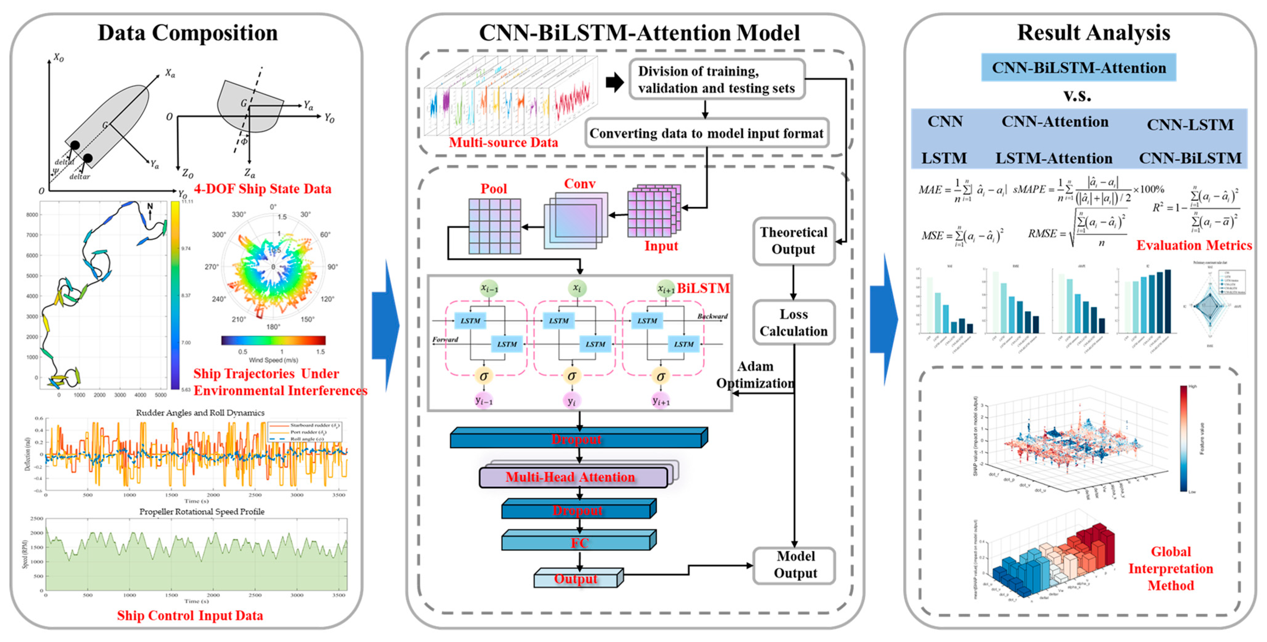
Finally, the objective of this study is to develop a multi-input–multi-output (MIMO) 4-DOF ship maneuvering model. In addition to comparing the ship state forecasting performance and ship trajectory prediction performance of various deep learning methods, it is also necessary to conduct an interpretability analysis of this “black box.” The methods studied in this research effectively provide explanations for ship state forecasting. In the context of predicting the 4-DOF maneuvering motion model of a ship under wind interference, the methods demonstrate enhanced expressive capabilities and higher prediction accuracy, exhibiting robust environmental adaptability. Table 1 List of symbols summarizes the main symbols, parameters, and variables used in this study. As shown in Figure 1, the main contributions of this study are as follows:

Table 1. List of symbols.

Symbol	Physical Meaning/Description
$u,v,w$	Surge, sway, and heave velocities in the body-fixed coordinate system.
$p,q,r$	Rolling, pitching, and yaw rates representing angular velocities about the principal axes.
$\dot{u},\dot{v},\dot{p},\dot{r}$	Linear and angular accelerations corresponding to $u,v,p,r$.
$\varphi ,\theta ,\psi$	Roll, pitch, and yaw angles describing vessel attitude.
${\mathrm{delta},\mathrm{detla}}_t,\delta$	Rudder angle, deflection of the rudder from the neutral position controlling yaw motion.
$n$	Propeller rotational speed determining thrust magnitude.
$X,Y,K,N$	Hydrodynamic forces (surge, sway) and moments (roll, yaw) acting on the hull.
$m,I_x,I_z$	Ship mass and moments of inertia about the longitudinal and vertical axes.
$V_w,alph{a}_t({\alpha }_x,{\alpha }_y)$	True wind speed and relative wind angle acting on the vessel.
$f(\cdot )$	Nonlinear mapping function approximated by the deep learning model.
$W,b$	Trainable weight matrices and bias vectors in each neural network layer.
$h_t,c_t$	Hidden and cell state vectors in LSTM/BiLSTM units representing temporal dependencies.
$Q,K,V$	Query, key, and value matrices used in the multi-head attention mechanism.
$MAE,RMSE,sMAPE,R^2$	Evaluation metrics measuring absolute, relative, and overall prediction accuracy.
${\Phi }_i$	SHapley value of feature i, indicating its contribution to the model’s output.
$S$	Set of all features considered in SHAP computation.
${\varphi }_i$	Marginal contribution of feature i to model prediction, computed by game-theoretic averaging.

Figure 1. The framework of the proposed method.

(1)

A hybrid model combining convolutional neural networks, bidirectional long short-term memory networks, and attention mechanisms was proposed and applied to the nonparametric system identification of ship motion.

(2)

The predictive capability of the model can be enhanced by incorporating environmental factors and additional historical factors as inputs, based on traditional ship operation motion models.

(3)

The proposed CNN-BiLSTM-Attention model was compared with the current mainstream deep learning models CNN, LSTM, LSTM-Attention, CNN-LSTM, and CNN-BiLSTM, considering four evaluation metrics: MAE, sMAPE, RMSE, and R2.

(4)

A coupled CNN-BiLSTM-Attention model employing SHapley Additive exPlanations (SHAP) technology was adopted to predict ship motion processes and identify key input feature factors for global interpretation and analysis.

2. The Construction of a MIMO Ship Maneuvering Motion Model

This section presents a comprehensive overview of the construction process for a MIMO ship maneuvering motion model. It encompasses the establishment of a traditional four-degree-of-freedom ship maneuvering model and the fundamental principles of the nonparametric system identification method proposed in this study. The method involves the utilization of a CNN-BiLSTM-Attention deep learning network and associated network components, as well as comparison algorithms, among other components.

2.1. An Introduction to the 4-DOF Ship Maneuvering Motion Model

The establishment of a ship maneuvering motion model is based on two systems: the ship coordinate system and the global coordinate system. A ship in motion at sea exhibits six degrees of freedom. The establishment of a mathematical model for ship maneuvering necessitates the construction of a reference coordinate system that describes the relevant motion variables of the ship, as illustrated in Figure 2.

Figure 2. The ship’s inertial coordinate system and body-fixed coordinate display. (a) presents a schematic representation of the six degrees of freedom of movement of a ship, while (b,c) show schematic representations of the four degrees of freedom of movement of a ship.

$O_0-X_0{Y}_0{Z}_0$ is representative of the inertial coordinate system, while $O-XYZ$ is representative of the body-fixed coordinate system. The arbitrary motion of a vessel in six degrees of freedom is described relative to a body-fixed coordinate system rigidly attached to the ship hull, with its origin typically at the center of gravity. This system defines six motion components that describe the vessel’s dynamics in the body-fixed coordinate frame. Specifically, the surge velocity ($u$), sway velocity ($v$), and heave velocity ($w$) denote the linear translational velocities along the longitudinal, transverse, and vertical axes, respectively. The rolling rate ($p$), pitching rate ($q$), and yaw rate ($r$) represent the angular velocities about these axes. These six components collectively describe the vessel’s three-dimensional motion state. In the inertial coordinate system, the motion state of a ship can be described using the Cartesian coordinates ${[x,y,z]}^T$ and the attitude angles ${[\varphi ,\theta ,\psi ]}^T$. It is important to note that ships exhibit underactuation, which necessitates the degradation or linearization of the system model during ship motion control design. The establishment of a ship maneuvering motion model involves the selection of appropriate degrees of freedom based on requirements, typically as follows:

One-degree-of-freedom models are employed in the design of ship forward speed control and heading control systems.

The design of 3-degree-of-freedom models can be further subdivided into numerous types, with the most prevalent being the planar motion model, which encompasses surge, sway, and yaw. A 4-degree-of-freedom model is predicated on the 3-degree-of-freedom planar motion model, with the incorporation of a rolling motion equation, as illustrated in Figure 2c. In this figure, the hull rotates around the $X_O$ axis, which is perpendicular to the $Y_O$-$Z_O$ plane.

Six degrees of freedom are frequently employed in the prediction of ship maneuvering performance, with a predominant application in various types of ship maneuvering simulators. In view of the acknowledged effect of wind on ship motion, the 4-DOF description of ship motion states is advantageous in that it offers both high accuracy and low computational complexity. In consideration of the geometric symmetry inherent in conventional hull forms, the pitch and heave motions exhibit a weak coupling with lateral and yaw motions. Consequently, these motions can be neglected without compromising the overall integrity of the analysis. The dynamic relationships of 4-DOF ship motion are described in Equation (1).

$$\left\{\begin{array}{l}m\left(\dot{u}-vr-x_G{r}^2+z_{G}pr\right)=X\hfill \\ m\left(\dot{v}+ur+x_G\dot{r}-z_G\dot{p}\right)=Y\hfill \\ I_{xx}\dot{p}-m{z}_G\left(\dot{v}+ur\right)=K\hfill \\ I_{zz}\dot{r}+m{x}_G\left(\dot{v}+ur\right)=N\hfill \end{array}\right.$$

(1)

In this system, $X,Y,K$ and $N$ represent the corresponding force components, roll and yaw moment, respectively. These forces and moments represent the external actions acting on the vessel, which collectively determine its motion states and are influenced by control commands. These functions are characterized by their high degree of complexity, nonlinearity, and multi-variable structure. In this framework, $m$ signifies the vessel’s mass, while $X_G,Y_G$ denote the coordinates of the ship’s center of gravity within the specified reference frame. $I_{xx}$ and $I_{zz}$ represent the moments of inertia of the ship’s mass with respect to the x and z axes, respectively. Firstly, it is evident that the inputs and outputs can be designated as the ship’s surge velocity, sway velocity, yaw rate, and roll rate (${[u,v,p,r]}^T$) and accelerations (${[\dot{u},\dot{v},\dot{p},\dot{r}]}^T$), in conjunction with the ship’s rudder angle and propeller speed. This configuration constitutes the conventional 4-DOF ship maneuvering motion model. Equation (1) is reformulated into Equation (2) to express the 4-DOF dynamics concisely, where the nonlinear function $F\left(·\right)$ encapsulates the coupled interactions among motion states, control inputs, and environmental forces. Here, ${[detla,n]}^T$ represent the rudder angle and propeller speed, with the yaw rate r fully characterizing heading dynamics through its time integral $\psi ={\displaystyle \int rdt}$.

$${[\dot{u},\dot{v},\dot{p},\dot{r}]}^T=F\left(\begin{array}{c}{[u,v,p,r]}^T\\ {[delta,n]}^T\end{array}\right)$$

(2)

Based on Equation (2), environmental disturbance forces are incorporated into this nonlinear system. The marine environment exerts a multifaceted influence on the motion state of a vessel, with its dynamic changes directly determining the vessel’s stability, safety, and operational efficiency. We selected wind as the representative factor in our analysis, given the well-known saying, “No wind, no waves.” In the context of wind interference, our analysis is constrained to the two-dimensional horizontal characteristics of wind, namely wind speed $v_w$ and wind direction. To more accurately assess wind interference on a vessel, the wind direction angle must be transformed into the angle at which the vessel is subjected to wind interference relative to the vessel’s wind angle, denoted by $\alpha$.

$${[\dot{u},\dot{v},\dot{p},\dot{r}]}^T=F\left(\begin{array}{c}{[u,v,p,r]}^T\\ {[delta,n]}^T\\ {[v_w,alpha]}^T\end{array}\right)$$

(3)

It is evident that historical data are characterized by their continuity and direct impact on the motion state of a vessel. This data encompasses the motion patterns exhibited by the vessel under various environmental conditions. The analysis of time series data facilitates the extraction of the inertial motion patterns of the vessel, including periodic swaying, acceleration or deceleration trends, and nonlinear characteristics. The variables in Equation (3) are transformed into fixed-length sliding window features (e.g., historical data from the past 1 s, 5 s, 10 s, and 50 s) to provide time-dependent input for the deep neural network. As demonstrated in Equation (4), the historical data point $histor{y}_t$ is employed as a component of the input to construct a MIMO ship maneuvering motion model.

$${[\dot{u},\dot{v},\dot{p},\dot{r}]}^T=F\left(\begin{array}{c}{[u,v,p,r]}^T\\ {[delta,n]}^T\\ {[v_w,alpha]}^T\\ histor{y}_t\end{array}\right)$$

(4)

2.2. The Construction of Deep Learning Networks

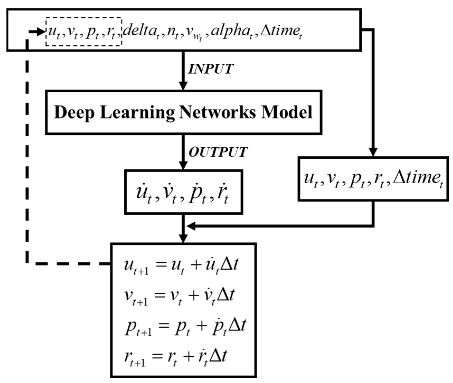
In accordance with the principles of deep learning neural network theory, when furnished with adequate and pertinent training data, these models possess the capacity to efficiently fit linear and nonlinear equations under the guidance of data. Therefore, deep neural networks can serve as an alternative to the nonlinear function $F\left(·\right)$ in Equation (4), as demonstrated in Figure 3. This section will commence with an introduction to the fundamental principle equations of a solitary network architecture model. Thereafter, a proposal for a composite network will be put forth.

Figure 3. Input and output of deep learning models.

2.2.1. Convolutional Neural Network Model

Convolutional neural networks (CNNs) have seen extensive application in various research domains and industrial projects [30]. The fundamental composition of a CNN comprises an input layer, convolutional layers, pooling layers, fully connected layers, and an output layer [31]. As illustrated in Figure 4, the convolutional layers and pooling layers are generally configured as multiple instances, arranged in an alternating pattern. In this pattern, a convolutional layer is connected to a pooling layer, followed by another convolutional layer, and this sequence repeats. In the convolution layer, each neuron in the output feature map is locally connected to its inputs. The weighted sum of the local inputs, multiplied by the corresponding connection weights, is added to the bias value to obtain the input value of the neuron. This process is analogous to the convolution process, which is the basis for the nomenclature of CNNs.

Figure 4. The structure of the convolutional neural network module.

CNNs possess several salient characteristics that have attracted the attention of many researchers, including local connectivity, weight sharing, pooling operations, and multi-layer structures. CNNs have been demonstrated to reduce the number of weights that need to be trained through a process known as weight sharing, thereby decreasing the computational complexity of the network. Concurrently, the implementation of pooling operations endows the network with specific invariance properties, including translation invariance and scaling invariance, with respect to local transformations of the input. This enhancement in invariance capabilities consequently leads to an improvement in the generalization ability of the network [32]. CNNs have the capacity to directly input raw data into the network, thereby enabling implicit learning from the training data. This process obviates the drawbacks associated with manual feature extraction, which can result in the accumulation of errors. The classification process is entirely automated.

2.2.2. LSTM and BiLSTM Model

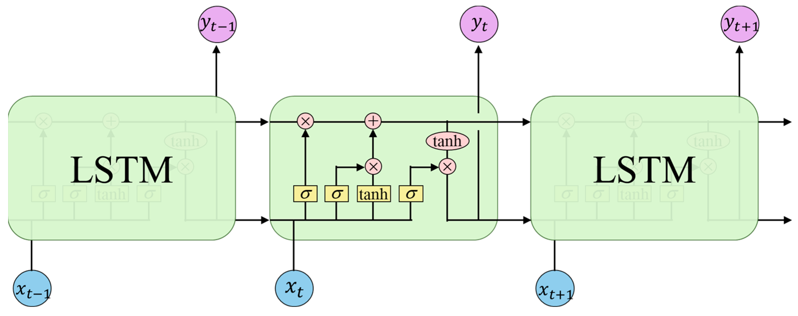
LSTM represents an enhancement to the neural network structure of RNNs, as illustrated in Figure 5. RNNs can process inputs of variable temporal lengths. However, as the quantity of inputs increases, RNNs become susceptible to issues such as gradient disappearance and gradient explosion. Hochreiter et al. [31] proposed the long short-term memory network, which aims to improve the traditional recurrent neural network model. LSTM has emerged as the most efficacious sequence model in practical applications. In comparison to the hidden units of RNNs, the internal structure of LSTM hidden units is more intricate. When information flows through the network, LSTM selectively amplifies or reduces information by introducing linear interventions, ensuring that the information processing of units at the current iteration time maintains strong temporal relevance with distant historical information.

Figure 5. Framework of LSTM model.

According to the LSTM structure depicted in Figure 5, $x_t$ and $y_t$ represent the input and output, respectively, while ${\tilde{C}}_t$ serves as the storage unit. The implementation of a nonlinear conversion gate structure is predicated on the utilization of distinct weight matrices $W$ and bias terms $b$, in accordance with the sigmoid function $\sigma \left(·\right)$. The expressions for each gate and memory cell in the gate mechanism and the storage unit ${\tilde{C}}_t$ are provided in Equation (5) and Equation (6), respectively:

$$\left\{\begin{array}{l}Forge{t}_t=\sigma (W_{forget}[H_{t-1},X_t]+b_{forget})\hfill \\ Inpu{t}_t=\sigma (W_{input}[H_{t-1},X_t]+b_{input})\hfill \\ Outpu{t}_t=\sigma (W_{output}[H_{t-1},X_t]+b_{output})\hfill \end{array}\right.$$

(5)

$$\widetilde{C_t}=\varphi (W_C[H_{t-1},X_t]+b_C)$$

(6)

The opening and closing of the input, output, and forget doors serve to regulate the flow of information. This results in outputs that are based on the unit status, and the final output is equal to Equation (7).

$$Y_t=Outpu{t}_t\varphi (\widetilde{C_t})$$

(7)

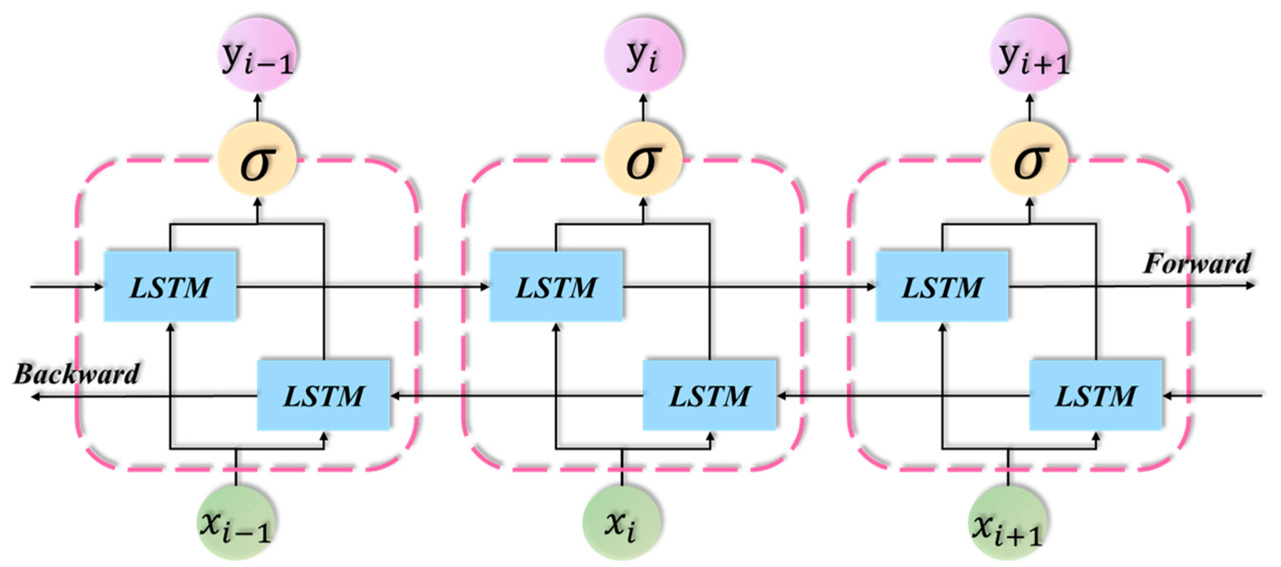
While LSTM addresses the shortcomings of RNNs, such as gradient explosion, it does not leverage information from sequences in the opposite direction during training. Consequently, it is unable to fully utilize time series data. This limitation is magnified to an infinite degree in complex ship motion states [24]. The BiLSTM model was proposed as a solution to these issues. The structure under consideration is a combination of forward and backward double-loop structures, as illustrated in Figure 6.

Figure 6. Framework of BiLSTM model.

From a temporal perspective, the BiLSTM network augments the unidirectional data flow from the past to the future in the LSTM network by introducing a bidirectional data flow from the future to the past. Furthermore, the absence of a connection between the hidden layers that act on the past and those that act on the future enables the BiLSTM network to more effectively capture temporal features in the data. In various application domains, the BiLSTM model has been shown to outperform conventional unidirectional LSTM models in terms of performance [33,34]. The BiLSTM model possesses a distinctive operational mechanism, thus allowing it to traverse the input data twice—initially from left to right and subsequently from right to left—thereby more effectively capturing underlying contextual information.

2.2.3. Multi-Head Attention Mechanisms

Multi-head attention represents a refinement of conventional attention mechanisms, as illustrated in Figure 7. It enhances the model’s expressive and learning capabilities by dividing the input features into multiple “heads,” with each head processing data independently [35]. In the multi-head attention mechanism, each element of the input sequence is mapped to three distinct vector spaces, referred to as the key ($K$), query ($Q$), and value ($V$) vectors.

Figure 7. The framework of multi-head attention mechanisms.

Research has demonstrated that, in comparison with the approach of calculating attention exclusively for $K$, $Q$, and $V$ with single attention, effectiveness is enhanced by learning multiple mappers through the model and executing multiple linear mappings for each dimension of $K$, $Q$, and $V$, as illustrated in Equations (8) and (9).

$$MultiHead(Q,K,V)=Concat(hea{d}_1,\dots ,hea{d}_h)W^O$$

(8)

$$\begin{array}{ll}hea{d}_i=& Attention(Q{W}_i^Q,K{W}_i^K,V{W}_i^V)\\ & W_i^Q\in {ℝ}^{d_{\mathrm{mod}el}\times d_k},W_i^K\in {ℝ}^{d_{\mathrm{mod}el}\times d_k},W_i^V\in {ℝ}^{d_{\mathrm{mod}el}\times d_k},W_i^O\in {ℝ}^{d_{\mathrm{mod}el}\times d_k}\end{array}$$

(9)

The incorporation of an attention mechanism within a neural network has been demonstrated to facilitate the network’s capacity to capture global dependencies with greater effectiveness, enhance the model’s selective attention capabilities, augment its parallelization capabilities, and fortify its expressive capabilities, among other advantages [36,37]. The utilization of attention mechanisms has been demonstrated to exert a favorable influence on neural networks.

2.2.4. CNN-BiLSTM-Attention Model

The model structure can be analyzed as shown in Figure 8 by combining a CNN with BiLSTM and then adding a multi-head attention mechanism. The CNN layer effectively reduces the dimension of the input data and enhances feature extraction capabilities through convolution operations performed by convolution kernels and down-sampling processes implemented by pooling layers. The BiLSTM layer has been shown to have significant advantages in terms of processing time series data. It has been demonstrated to be effective in capturing the long-term dependencies between dynamic features and navigation state features in time series data. BiLSTM comprises two LSTM units that operate in opposite directions, with each unit responsible for processing information in a specific direction. This enables the model to concurrently acquire information from both preceding and subsequent time steps, thereby facilitating a more comprehensive understanding of dynamic alterations in the sequence. CNN-BiLSTM integrates the strengths of both models, leveraging their complementarity. The incorporation of a multi-head attention mechanism enhances the model’s learning and expressive capabilities by capturing data diversity from multiple perspectives through the parallel processing and integration of attention heads.

Figure 8. The framework of CNN-BiLSTM-Attention.

3. SHapley Additive exPlanations Technology

Machine learning and deep learning have achieved considerable success in a variety of applications; however, their lack of interpretability significantly restricts their use in real-world scenarios, particularly those that are critical to safety. The present study focuses on the application of the SHAP interpretable method in a deep learning-based ship maneuvering motion model. SHAP is a post hoc explanation framework that is based on game theory [38] and local explanations [39]. It provides Shapley values to assess the contribution of each feature. Shapley values are utilized to ascertain the marginal contribution of each feature to the model’s prediction outcomes, as expressed by the following mathematical formulation:

$${\varphi }_i(v)=\sum _{S\subseteq N\setminus \left\{i\right\}}{\displaystyle \frac{\left|S\right|!(|N|-|S|-1)!}{\left|N\right|!}}\left[v(S\cup \{i\})-v(S)\right]$$

(10)

In this context, $!$ denotes the factorial operation, $N$ denotes the set of all features, and $S$ denotes the subset of features that does not include feature $i$. $v\left(S\right)$ represents the predicted value on the feature subset $S$, and ${\varphi }_i\left(v\right)$ denotes the contribution of the feature to the prediction result, i.e., the Shapley value. This is the core of SHAP. In comparison to conventional feature importance methodologies, SHAP has been demonstrated to exhibit enhanced consistency, as it facilitates the representation of the positive/negative relationship between each predictor and the target variable. Furthermore, SHAP can be utilized for both local and global interpretation [40]. With respect to local interpretability, it is important to note that each feature has its own set of Shapley values. Consequently, this approach can be employed to elucidate the contribution of each feature to the prediction for each sample, thereby enhancing transparency and facilitating the analysis of the reliability of the predictive model. In addition, the visual results obtained from SHAP analysis are especially useful for interpreting models, as demonstrated in Figure 9. A comprehensive explanation and clarification of the global interpretation of the model will be provided in the subsequent sections of this paper.

Figure 9. Global explanation and analysis diagram of SHAP technology.

4. Experimental Data and Design

This section provides a comprehensive overview of the preliminary phase of the experiment and its components, encompassing the composition of experimental data, the determination of the historical dimensions of input data, and the selection of evaluation indicators and related algorithm parameters, as well as environmental parameters.

4.1. Composition of Experimental Data

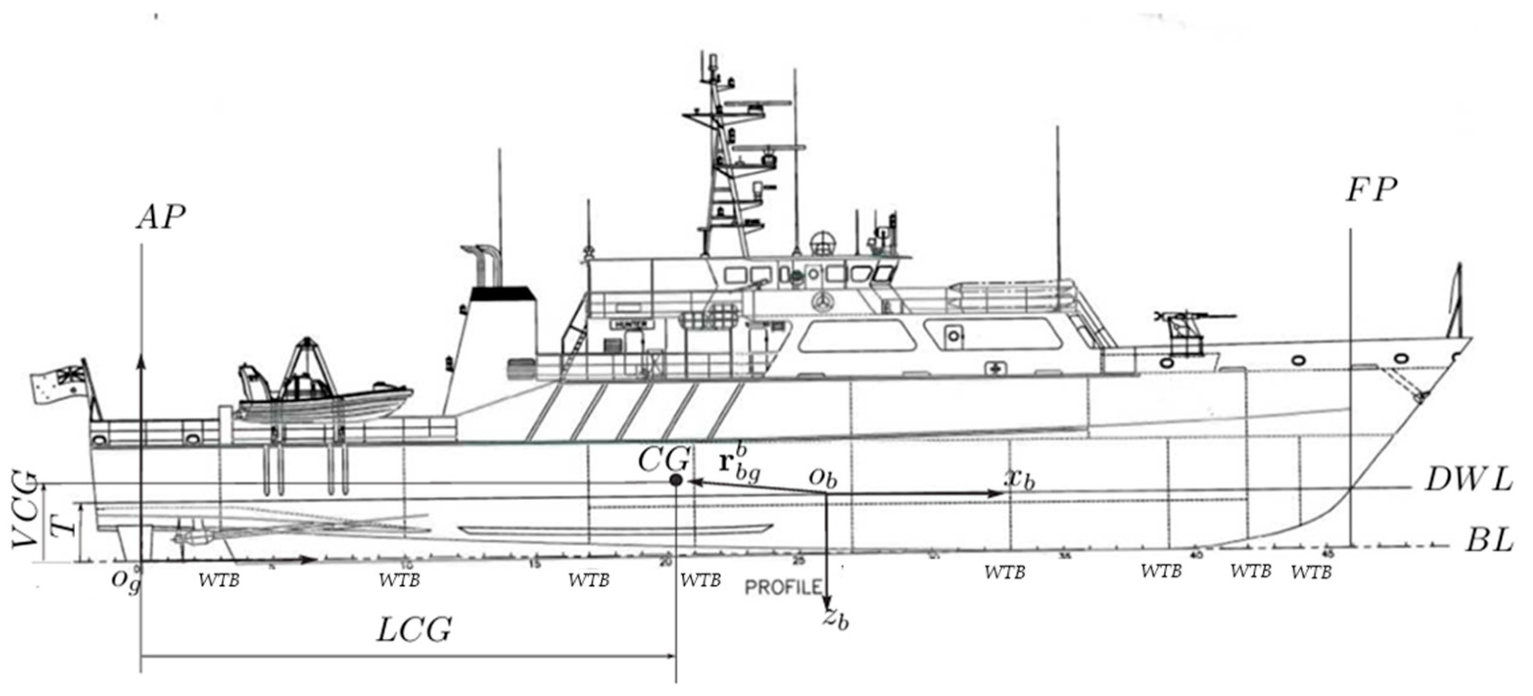
The experimental data presented in this study were obtained from [41]. A single-rudder, single-propeller patrol boat based on [42]’s design was developed. The original patrol boat was modified and expanded with the addition of a set of symmetrically placed propellers and a rudder, as illustrated in Figure 10. Furthermore, the environmental effects on the vessel’s motion were simulated using Isherwood’s wind model [43] to generate wind forces. The generation of wind-induced waves was accomplished through the utilization of the JONSWAP spectrum [44], and the subsequent calculation of wave forces was performed employing the wave force response amplitude operator (RAO).

Figure 10. Image of patrol boat proposed by Perez et al. [42].

The dataset under consideration contains 125 sets of data simulating ship motion for one hour in various sea states while performing random maneuvers in 4 degrees of freedom (surge–sway–yaw–roll). All motion states were sampled at 1 Hz, thus corresponding to the characteristic periods of ship dynamics. The conventional dataset is divided into training, testing, and validation sets in a 6:3:1 ratio, totaling 96 h. Furthermore, the analysis of the final results will also utilize the 29 h of data not included in the conventional dataset. Figure 11 displays the complete path of a single motion in the non-conventional dataset, along with scatter plots of wind speed and direction in polar coordinates and control input diagrams during the simulated voyage. The trajectory is depicted with uniform plotting, with the initial vessel coordinates designated as (0,0).

Figure 11. Dataset visualization, including ship trajectory maps, wind speed and direction maps, and control input maps.

4.2. Evaluation Indicators

The evaluation of a model’s performance is conducted from two complementary perspectives. Firstly, the model’s intrinsic predictive capability is validated. Secondly, its effectiveness is compared against that of alternative methods. The present study adopts a range of four metrics used to comprehensively quantify predictive accuracy and global fit quality. The four metrics employed are as follows: the mean absolute error ($MAE$), symmetrical mean absolute percentage error ($sMAPE$), root mean square error ($RMSE$), and the coefficient of determination ($R^2$). The $MAE$ is a metric used to quantify the average absolute deviation between the values predicted by a model and the actual values. Smaller values indicate higher precision. The $RMSE$, on the other hand, is a metric that emphasizes larger errors by squaring the residuals, thereby highlighting the model’s sensitivity to extreme deviations. However, the traditional $MAPE$ is susceptible to distortion when actual values approach zero (e.g., low-speed ship maneuvers), thus resulting in biased error statistics. To address this issue, the $sMAPE$ normalizes errors by using the sum of predicted and actual values, thereby reducing bias in scenarios in which the errors are near zero. Concurrently, $R^2$ quantifies the proportion of variance explained by the model, with values approaching 1 denoting superior global fit. The integration of absolute error, relative error, and global fit metrics within the evaluation framework ensures the capture of both localized error distributions and overall trend consistency. This approach guarantees robust and comprehensive results. The following mathematical expressions are utilized to calculate the aforementioned evaluation metrics:

$$MAE={\displaystyle \frac{1}{n}}\sum _{i=1}^n\mid {\hat{y}}_i-y_i\mid ,$$

(11)

$$sMAPE={\displaystyle \frac{1}{n}}\sum _{i=1}^n{\displaystyle \frac{\left|{\widehat{y}}_i-y_i\right|}{\left(\left|{\widehat{y}}_i\right|+\left|y_i\right|\right)/2}}\times 100\%,$$

(12)

$$RMSE=\sqrt{\frac{{\displaystyle \sum _{i=1}^n}{\left({\widehat{y}}_i-y_i\right)}^2}{n}},$$

(13)

$$R^2=1-\frac{{\displaystyle \sum _{i=1}^n}{\left({\widehat{y}}_i-y_i\right)}^2}{{\displaystyle \sum _{i=1}^n}{\left(y_i-\overline{y}\right)}^2}$$

(14)

In this context, for the $i$-th data point in the evaluation set, $y_i$ denotes the observed value of vessel dynamic parameters, ${\widehat{y}}_i$ represents the model’s predicted value, and $\overline{y}$ is the arithmetic mean of all $y_i$. To assess the performance differences between the CNN–BiLSTM–Attention model and other algorithms in a more intuitive manner, the following improvement rates are defined: $E_{MAE}$, $E_{sMAPE}$, $E_{RMSE}$, and $E_{R^2}$ [26]. The detailed mathematical expressions are shown below. When their value is greater than 0, it indicates that the method proposed in this paper is superior to the comparison algorithms. $MA{E}_{IM}$, $sMAP{E}_{IM}$, $RMS{E}_{IM}$, and $R_{IM}^2$ represent the evaluation metrics corresponding to the method proposed in this study, while $MA{E}_{CA}$, $sMAP{E}_{CA}$, $RMS{E}_{CA}$, and $R_{CA}^2$ represent the evaluation metrics corresponding to the comparison algorithms.

$$E_{MAE}=({\displaystyle \frac{MA{E}_{CA}-MA{E}_{IM}}{MA{E}_{CA}}})\times 100\%,$$

(15)

$$E_{sMAPE}=({\displaystyle \frac{sMAP{E}_{CA}-sMAP{E}_{IM}}{sMAP{E}_{CA}}})\times 100\%,$$

(16)

$$E_{RMSE}=({\displaystyle \frac{RMS{E}_{CA}-RMS{E}_{IM}}{RMS{E}_{CA}}})\times 100\%,$$

(17)

$$E_{R^2}=\left|{\displaystyle \frac{R_{CA}^2-R_{IM}^2}{R_{CA}^2}}\right|\times 100\%$$

(18)

4.3. Determination of Historical Data Dimensions

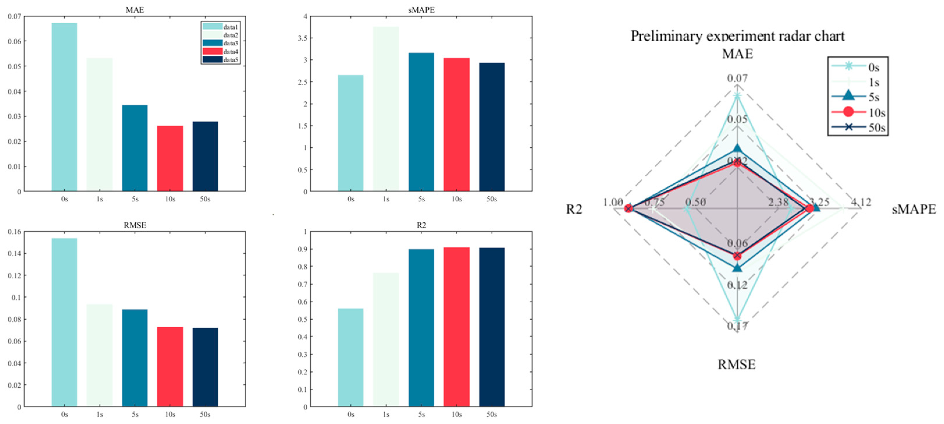
As previously mentioned, the construction of fixed-length sliding window features provides time-dependent input for deep neural networks. The selection of an appropriate historical data dimension is beneficial for improved prediction. Specifically, we conducted a preliminary experiment utilizing a single hour of data for training, testing four distinct durations (1 s, 5 s, 10 s, and 50 s) of past ship movement history, and a scenario lacking historical data. The effects of these durations on the model performance of the deep learning network were then compared. The results of the preliminary experiment were exclusively employed as a reference point for the determination of the historical data dimension. As demonstrated in Table 2 and Figure 12, the performance of the aforementioned algorithm is shown to vary with different historical data dimensions on the training set.

Table 2. Indicators of preliminary experiment evaluation results.

Items	MAE	sMAPE	RMSE	${\mathit{R}}^2$
0 s	0.0670	2.6426	0.1533	0.5576
1 s	0.0531	3.7412	0.0932	0.7602
5 s	0.0344	3.1501	0.0884	0.8960
10 s	0.0260	3.0280	0.0725	0.9058
50 s	0.0276	2.9250	0.0717	0.9044

Figure 12. Visualization of preliminary experiment evaluation indicators.

As demonstrated in Table 2 and Figure 12, incorporating historical data significantly enhances model performance. As the historical window increases from 1 s to 10 s, there is a consistent improvement in the four evaluation metrics. This finding suggests that longer windows are better at capturing the dynamic characteristics of ship motion. However, extending the window to 50 s leads to performance fluctuations in some metrics and increased computational costs. Therefore, 10 s is adopted as the input length. This choice is based on two factors. Firstly, the typical response time scales of ship motion, such as rudder lag and wave excitation cycles, are usually in the order of seconds. This allows the 10 s window to balance dynamic modeling needs and efficiency. Secondly, experimental validation confirms that the 10 s window outperforms shorter or longer windows in most metrics.

5. Results and Discussion

This section is devoted to a comprehensive comparison of the CNN–BiLSTM–Attention model with other comparison algorithms. Four evaluation metrics are selected to assess the predictive capabilities of the CNN–BiLSTM–Attention model. The dataset used for model development consists of 125 one-hour simulations under various sea states, which are divided into training, validation, and testing sets in a 6:3:1 ratio, totaling 96 h of data. To further examine the model’s generalization ability, an additional 29 h non-conventional dataset, independent from the training process, is employed for external evaluation. The final stage of the process involves the implementation of the SHAP technique for global interpretation and analysis.

5.1. The Training Process

All experiments in this study were conducted on an Intel Core i9-14900KF CPU with 128 GB of DDR5 memory and an NVIDIA RTX 5080 graphics card with 16 GB of VRAM. The experimental code was executed on MathWorks’ MATLAB R2023b platform, utilizing the Deep Learning Toolbox for the design of deep learning neural networks. The Deep Learning Toolbox furnishes functions, applications, and Simulink modules for the design, implementation, and simulation of deep neural networks.

The present study employs the CNN-BiLSTM-Attention model to predict ship maneuvering movements, with each submodule of the model requiring reasonable design. This is because as the number of neurons increases, more training cycles are required, which in turn leads to an increase in training time. To achieve a balance between training time, model complexity, and model performance, this study references the work of other scholars [21,25] on deep learning network design, with specific parameters as shown in Table 3. The model employs the ReLU activation function, Adam optimizer, and MSE loss function. The number of epochs is set to 5000, with an initial learning rate of 0.001, which is adjusted to 0.0002 after 3000 iterations, and a batch size of 256. The model’s training is executed through the utilization of the Adam gradient descent algorithm, which is employed to optimize the loss function value. The Adam algorithm is a refined gradient optimization algorithm that has demonstrated its effectiveness in producing satisfactory results [45]. In comparison with classical algorithms, the Adam algorithm has demonstrated a substantial enhancement in computational efficiency and is well-suited for addressing optimization problems involving large-scale data and multiple parameters [46].

Table 3. Architecture and hyperparameters of the CNN–BiLSTM–Attention model.

Component	Configuration and Description
Input	$u,v,p,r,\mathrm{detla},n,V_w,alpha$ sampled at 1 Hz; historical time steps are used as sequential inputs.
CNN stack	Two Conv1D layers: filters [32, 64]; kernel size = 3; stride = 1; padding = “same”; each followed by ReLU and MaxPool (pool size = 2).
Temporal alignment	Feature maps flattened/reshaped into a time–feature sequence for recurrent processing.
BiLSTM	Two bidirectional LSTM layers; 128 hidden units per direction.
Multi-head self-attention	Number of heads = 3; key dimension = 6; attention weights computed with softmax.
Outputs	Predicted accelerations $[\dot{u},\dot{v},\dot{p},\dot{r}]$.
Loss	MSE.
Activation function	ReLU.
Optimizer	Adam.
Learning-rate schedule	Initial 0.001; reduced to 0.0002 after 3000 iterations.
Dropout	0.05.
Batch size	256.
Epochs	5000.

5.2. Comparative Experiments of Different Models

In this section, we undertake further comparative research, comparing the proposed method with several mainstream prediction models. Five mainstream deep neural network models are selected for comparison: CNN, LSTM, LSTM-Attention, CNN-LSTM, and CNN-BiLSTM. These models are used for time series prediction. The conventional datasets referenced in the preceding section are utilized for training, and their superiority and robustness are substantiated by comparing the prediction results with unconventional datasets.

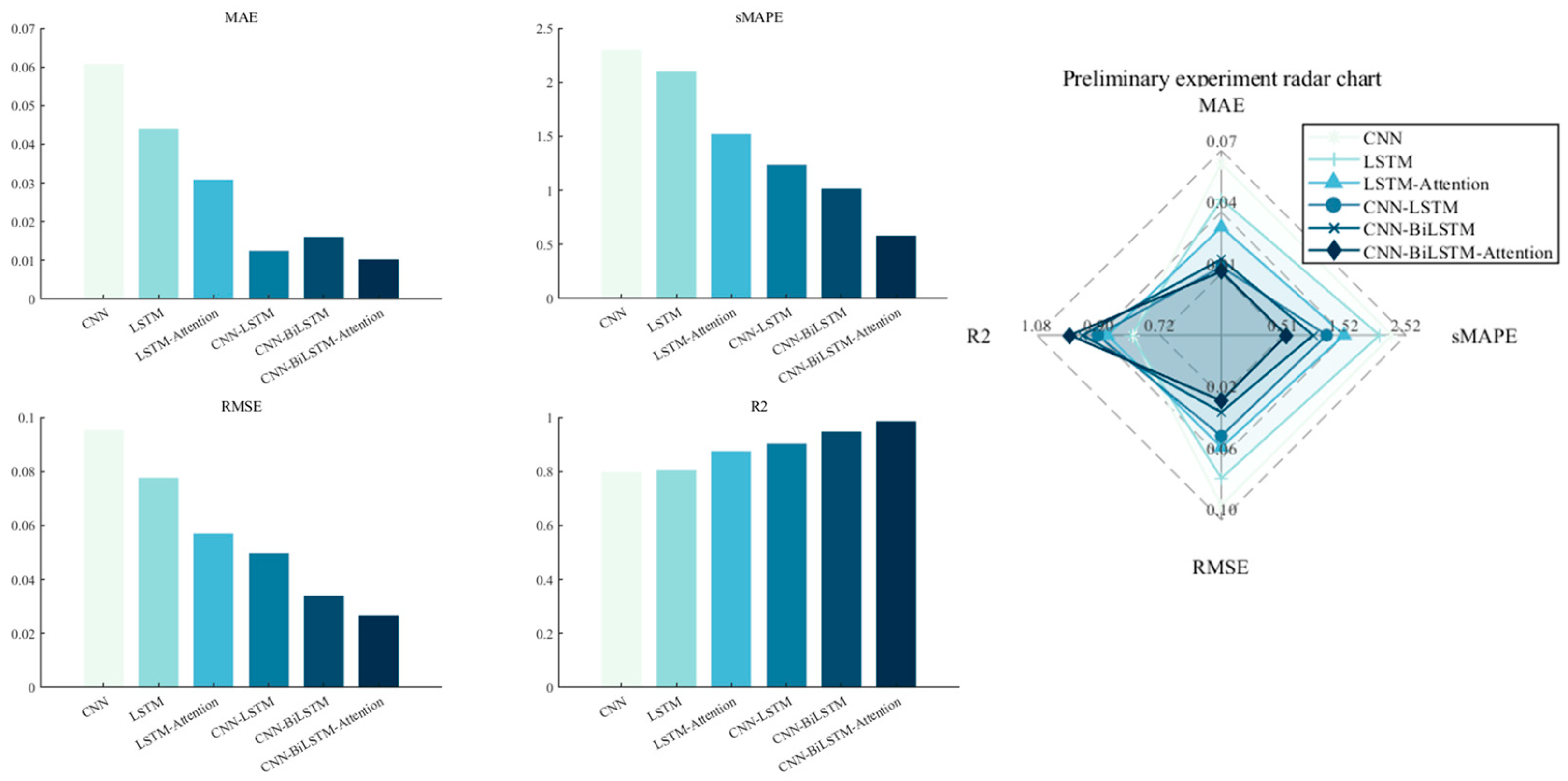
The proposed CNN-BiLSTM-Attention model was evaluated using five evaluation metrics, and its training performance on the conventional training set is shown in Table 4 and Figure 13. As demonstrated in Table 4, the CNN-BiLSTM-Attention model demonstrates superior performance across all metrics, exhibiting the lowest MAE and sMAPE values among all models. This finding suggests that the model attains the lowest average absolute discrepancy between predicted outcomes and actual values, thereby demonstrating optimal performance. The RMSE is a metric that quantifies the discrepancy between predicted and actual values. It exhibits heightened sensitivity to substantial errors. The CNN-BiLSTM-Attention model demonstrates the lowest values for both metrics, indicating that it not only exhibits the smallest average error but also performs optimally when handling samples with substantial errors. The R² value of the CNN-BiLSTM-Attention model is 0.983, which is the highest among all models, thus indicating the optimal fitting effect. Furthermore, single-architecture models demonstrate inferior performance in predicting ship maneuvering movements when compared to hybrid structure models. The CNN-BiLSTM-Attention model demonstrates remarkable effectiveness across all evaluation metrics, particularly in terms of reducing prediction errors and enhancing model interpretability.

Table 4. Effectiveness of different models in terms of four evaluation indicators.

	CNN	LSTM	LSTM- Attention	CNN-LSTM	CNN-BiLSTM	CNN-BiLSTM-Attention
$MAE$	0.0186	0.0188	0.0177	0.0158	0.0122	0.0099
$sMAPE$	1.1914	1.1903	1.1120	1.0269	1.0057	0.6708
$RMSE$	0.0418	0.0419	0.0409	0.0396	0.0338	0.0262
$R^2$	0.8368	0.8381	0.8718	0.900	0.9354	0.9829

Figure 13. Effectiveness of different models in terms of four evaluation indicators.

To further evaluate the enhanced predictive capabilities of the proposed method on a single prediction model, $E_{MAE}$, $E_{sMAPE}$, $E_{RMSE}$, and $E_{R^2}$ are calculated, and their values are presented in Table 5. As illustrated in this table, the proposed CNN-BiLSTM-Attention model was enhanced relative to the comparison model. A comparison with single-structure deep learning models is more significant, and the predictive performance was also improved compared with other hybrid structure models. A comparison with the CNN-BiLSTM model reveals that the proposed method achieves an 18.41% improvement in the MAE, a 33.30% improvement in the sMAPE, a 22.23% improvement in the RMSE, and a 4.8% improvement in R² by incorporating the multi-head attention mechanism.

Table 5. Improvement rate of CNN-BiLSTM-Attention over other models.

	CNN	LSTM	LSTM- Attention	CNN-LSTM	CNN-BiLSTM
$E_{MAE}$	46.46	46.86	43.74	36.78	18.41
$E_{sMAPE}$	55.34	43.65	39.67	34.69	33.30
$E_{RMSE}$	37.14	37.36	35.79	33.58	22.33
$E_{R^2}$	14.85	14.72	11.30	8.32	4.83

To achieve a more precise reflection of the model’s predictive performance beyond the confines of the training set, a comparison of its performance was conducted using unconventional datasets. As demonstrated in Table 6, under the unconventional training set, the proposed algorithm and the comparison algorithms were evaluated using four ship motion description variables: $u$, $v$, $p$ and $r$ This table compares the prediction performance of the CNN-LSTM, CNN-BiLSTM, and CNN–BiLSTM–Attention models across the variables using four metrics: the $MAE$, $sMAPE$, $RMSE$, and $R^2$. The data indicates that the CNN–BiLSTM–Attention model demonstrates the optimal performance across all metrics. In particular, the model’s mean absolute error ($MAE$) demonstrated a substantial decline, from 0.1620 in the CNN-LSTM configuration to 0.011. Concurrently, the R² metric exhibited a notable enhancement, increasing from 0.9027 to 0.9843. These observations suggest that the incorporation of an attention mechanism into the model design led to a substantial enhancement in its capacity to discern salient features. While CNN-BiLSTM demonstrated enhancements over the baseline model, its error rate remained at a higher level compared to the version incorporating a multi-head attention mechanism. The errors of the variable in question are generally higher than those of other variables, which may be related to the complexity of its data distribution.

Table 6. The validation of simulation data.

	CNN-LSTM				CNN-BiLSTM				CNN-BiLSTM-Attention
	$\mathit{u}$	$\mathit{v}$	$\mathit{p}$	$\mathit{r}$	$\mathit{u}$	$\mathit{v}$	$\mathit{p}$	$\mathit{r}$	$\mathit{u}$	$\mathit{v}$	$\mathit{p}$	$\mathit{r}$
MAE	0.0153	0.0156	0.0162	0.159	0.0122	0.0126	0.0131	0.0128	0.0095	0.0101	0.0112	0.099
sMAPE	1.0245	1.0232	1.0643	1.0336	1.0068	1.0078	1.0082	1.008	0.6843	0.7105	0.7522	0.6635
RMSE	0.0394	0.0391	0.0411	0.0392	0.0327	0.0333	0.0358	0.0347	0.0262	0.0268	0.0271	0.0265
R2	0.9193	0.9263	0.8942	0.9125	0.9308	0.9279	0.9187	0.9294	0.9844	0.9821	0.9819	0.9848

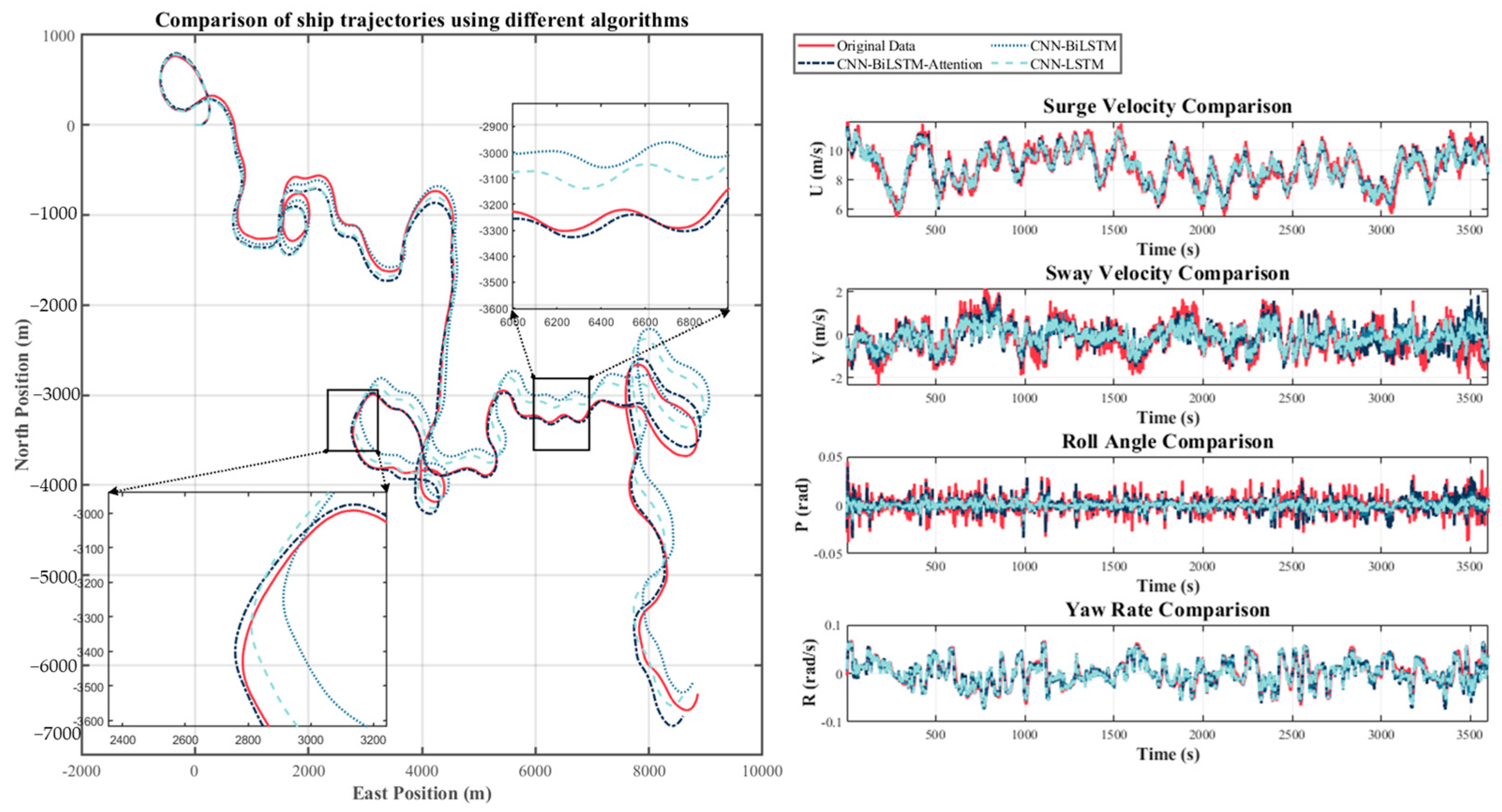
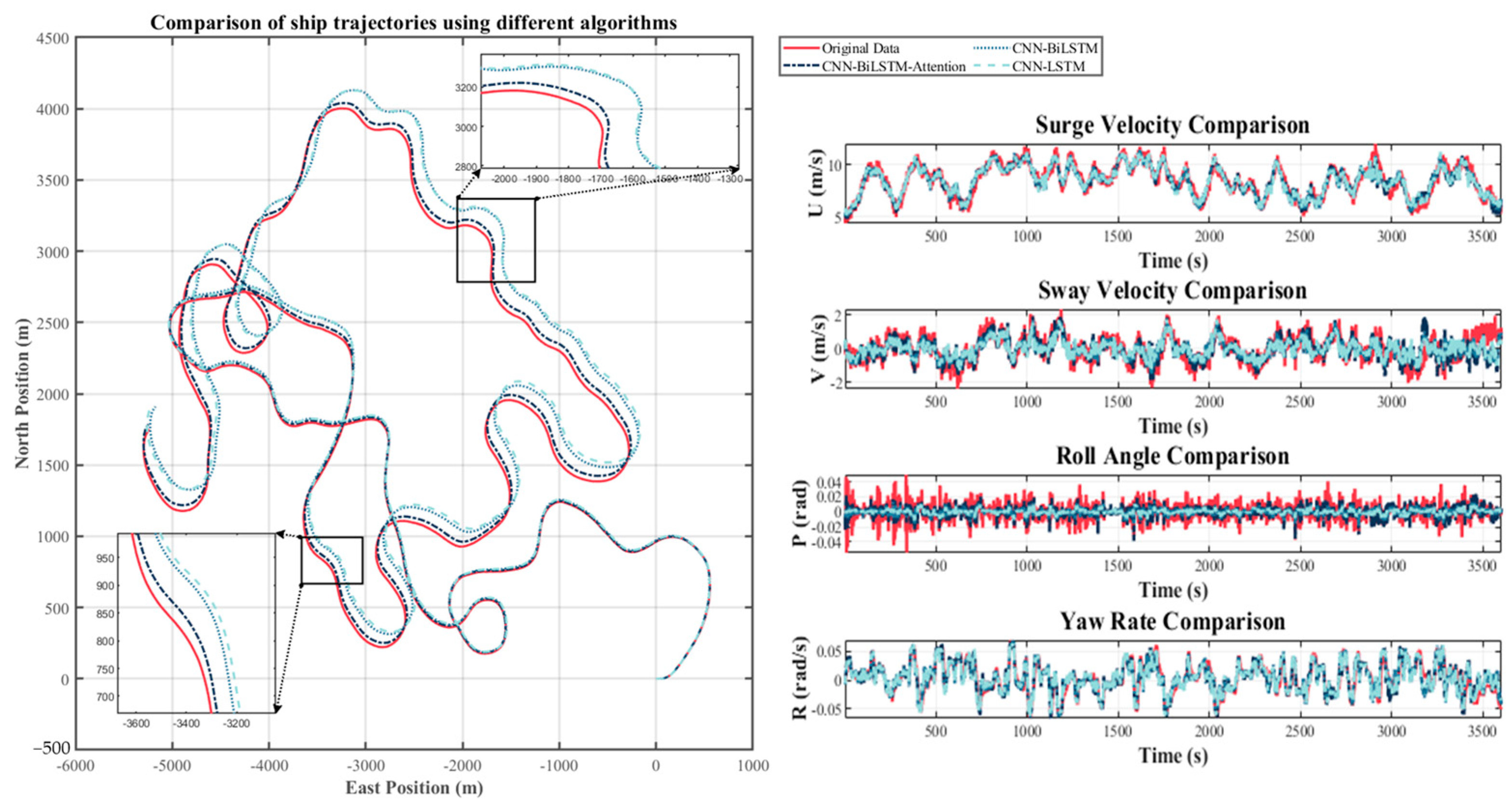
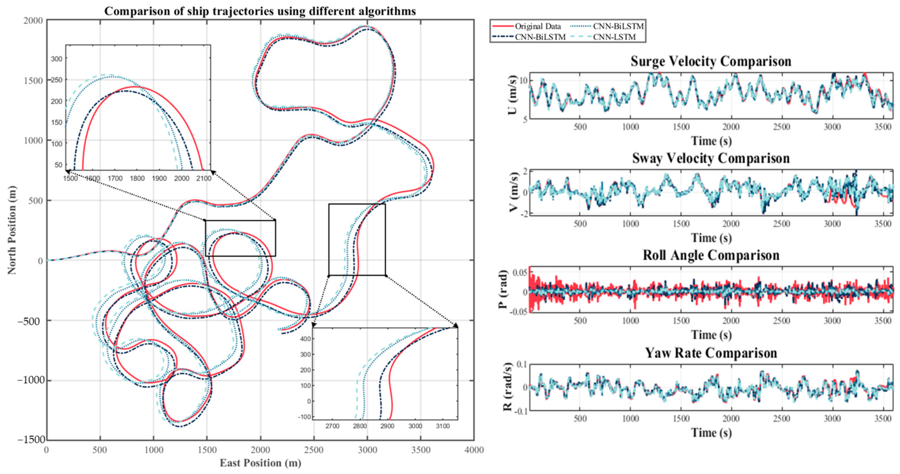
In this study, we will present the prediction performance for three distinct wind speed ranges: specifically, the velocity ranges were set at 0.5 m per second (m/s) to 2.5 m per second (m/s), 2.5 m per second to 5.0 m per second, and 3.5 m per second to 4.5 m per second. The trajectory plots are displayed in Figure 14, Figure 15 and Figure 16. The trajectory is obtained by performing two numerical integrations of the acceleration obtained from the model to determine the ship’s position and heading angle, thereby generating the trajectory. Figure 14 presents a comparison between the predicted trajectories and the actual trajectories for the wind speed range of 0.5 m/s to 2.5 m/s. Figure 15 also presents comparison plots of the four ship motion description variables ($u$, $v$, $p$ and $r$). The CNN-LSTM and CNN-BiLSTM models are utilized as references. Figure 16 presents a comparison between the predicted trajectories and the actual trajectories for wind speeds ranging from 3.5 m/s to 4.5 m/s, along with four comparison diagrams of ship motion description variables. As illustrated by the comparison diagrams, the CNN-BiLSTM-Attention model exhibited remarkable predictive effectiveness, aligning with the findings presented in Table 6. When confronted with varying wind speeds, the CNN-BiLSTM model demonstrated enhanced interference resilience in comparison to both the CNN-BiLSTM and CNN-LSTM models.

Figure 14. Predicted and actual trajectory comparison diagram under wind speeds ranging from 0.5 m/s to 2.5 m/s.

Figure 15. Predicted and actual trajectory comparison diagram under wind speeds ranging from 2.5 m/s to 5.0 m/s.

Figure 16. Predicted and actual trajectory comparison diagram under wind speeds ranging from 3.5 m/s to 4.5 m/s.

5.3. Global Interpretation and Analysis of Models

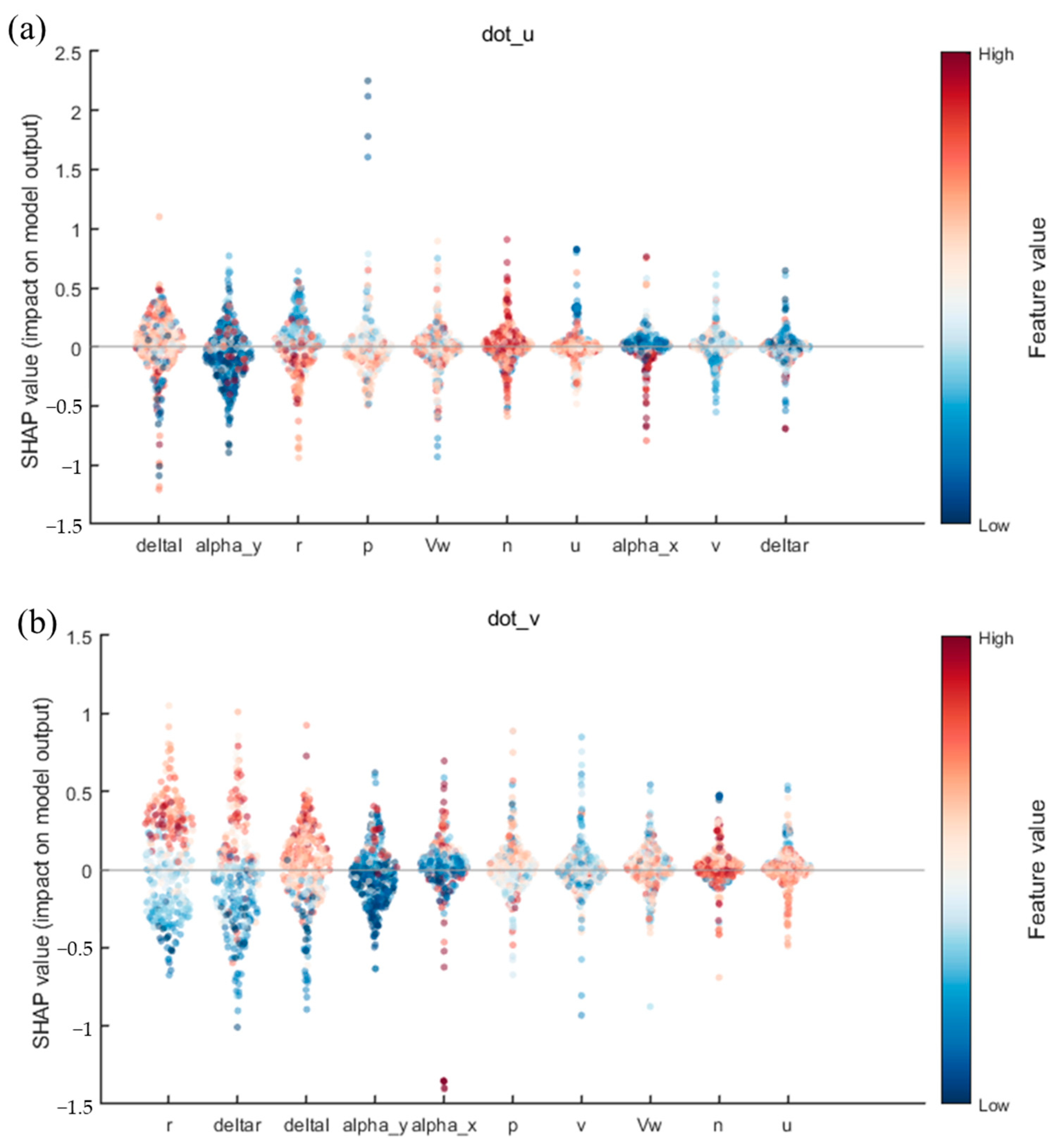
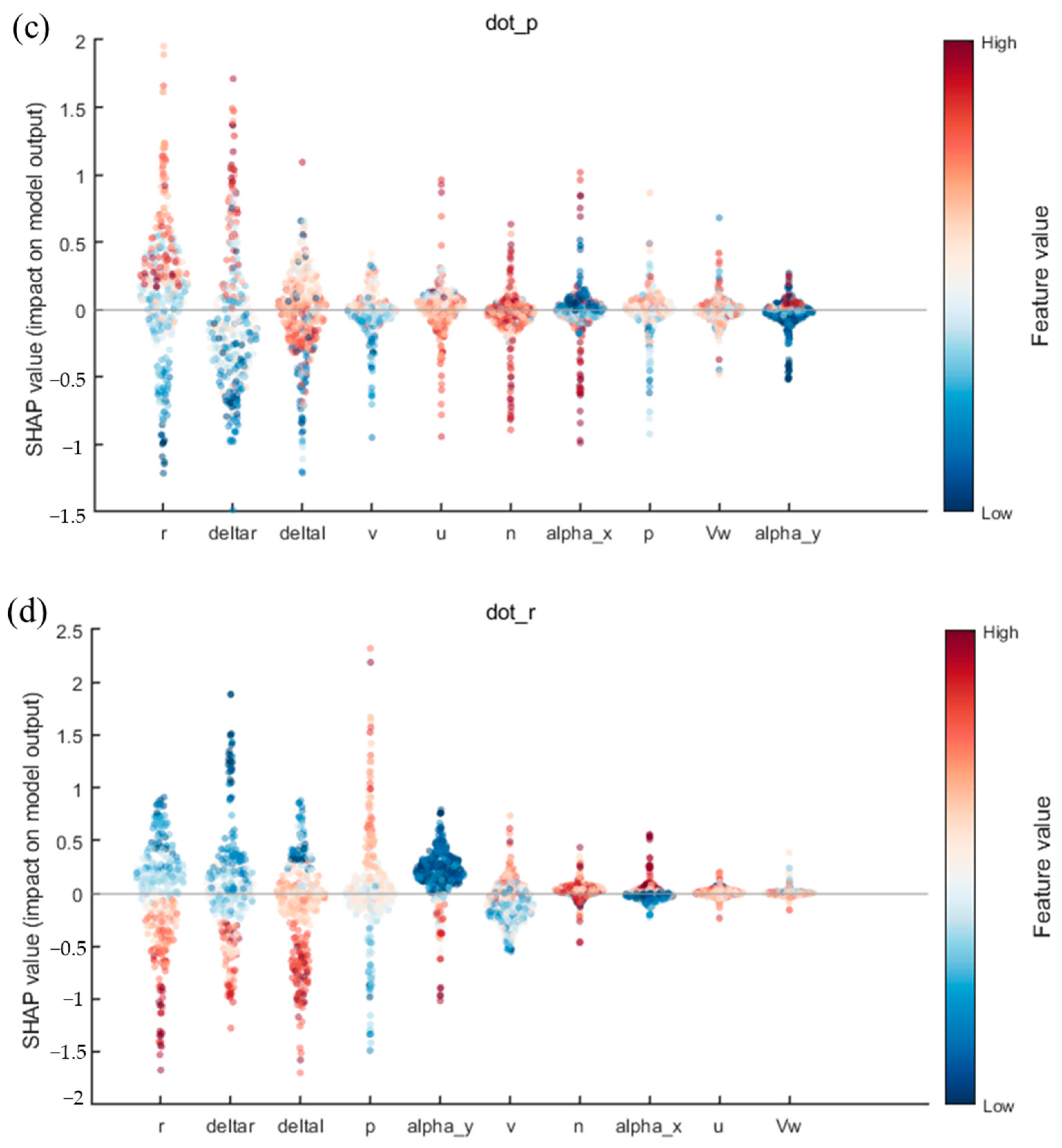
In this subsection, we will utilize SHapley Additive exPlanations technology to provide a comprehensive explanation of the CNN-BiLSTM-Attention model proposed in this paper. Furthermore, to demonstrate the impact of historical data as input on the output, we will also use SHAP on the black-box model when historical data are included as input. As demonstrated in Figure 17, in the absence of historical data (i.e., when considering Equation (3)), the inputs comprise the ship’s surge velocity, sway velocity, roll rate, and yaw rate (${[u,v,p,r]}^T$), as well as the ship’s rudder angle, propeller speed, wind speed, and wind angle, and the output is defined as the acceleration (${[\dot{u},\dot{v},\dot{p},\dot{r}]}^T$). In this figure, dot_u, dot_v, dot_p, and dot_r represent the predicted effects of surge acceleration ($\dot{u}$), sway acceleration ($\dot{v}$), roll angle acceleration ($\dot{p}$), and yaw angle acceleration ($\dot{r}$), respectively.

Figure 17. The ranking of factors influencing the ship’s maneuvering motion model based on the experimental results without historical data: (a) the influence of each feature on the prediction of surge acceleration ($\dot{u}$); (b) the influence of each feature on the prediction of sway acceleration ($\dot{v}$); (c) the influence of each feature on the prediction of bow roll angle angular velocity ($\dot{p}$); and (d) the influence of each feature on the prediction of yaw angle acceleration ($\dot{r}$).

SHAP plots have been demonstrated to reveal the influence of different features on the model output, as well as their directionality. In the dot_u model, the features delta and alpha_y exert a substantial positive influence on model prediction, particularly when feature values are elevated. Conversely, the effects of r and p are negligible and unstable. In the dot_v model, delta and alpha_x demonstrate a significant negative impact on output when feature values are high, while the effects of v and Vw are comparatively minimal. In the contexts of dot_p and dot_r, the variables deltar and deltas are found to be of pivotal significance. Specifically, deltar exerts a pronounced positive influence on output, particularly at elevated feature values in the dot_p scenario. Conversely, deltas demonstrates a negative correlation at reduced feature values in the dot_r setting. Furthermore, p and alpha_y exhibit a degree of influence in dot_r. In sum, deltar and deltal occupy a central position in all model outputs, with their directional changes directly linked to fluctuations in the model prediction results. The predominant role of p in dot_p and dot_r underscores its significance.

As demonstrated in Figure 18, following the incorporation of historical data, the factors influencing the output underwent substantial alterations. In this study, the top 15 features were selected based on their contribution to the output. An analysis of the SHAP plot reveals the critical role of historical data in model prediction, with its dynamic correlation and cumulative effect on time series features exerting a substantial influence on the stability and directionality of the model output. In the dot_u section, multiple historical time point features, represented by u and p, exhibit a pronounced driving effect on the model results. Changes in the feature values of certain specific historical stages directly determine the positive or negative bias of the output. In dot_r, the SHAP values of the deltar series features are highly concentrated and deviate from zero, thus indicating that historical difference features (e.g., fluctuations or trends between adjacent time points) are the primary source of model sensitivity. In dot_p and dot_v, the significant contribution of the v series and historical features such as u and p further underscores the supporting role of time series data in pressure and velocity prediction, with their distribution range and change direction directly influencing the model’s dynamic response. Overall, the model is highly dependent on historical data. The feature values at different time points are not only independent but also interact with each other, thereby increasing the complexity of the prediction results through mutual correlations. This finding underscores the significance of optimizing the quality of historical data inputs and capturing the evolutionary patterns of key time windows to enhance model robustness and interpretability.

Figure 18. The importance ranking of factors affecting the ship maneuvering motion model is as follows, as seen in the experimental results with historical data: (a) the influence of each feature on the prediction of surge acceleration ($\dot{u}$); (b) the influence of each feature on the prediction of sway acceleration ($\dot{v}$); (c) the influence of each feature on the prediction of roll angle acceleration ($\dot{p}$); and (d) the influence of each feature on the prediction of yaw angle acceleration ($\dot{r}$).

6. Conclusions

This study proposes a data-driven method that utilizes deep learning technology to address the non-systematic identification problem related to ship maneuvering motion models. Unlike previous studies, not only does the proposed method use traditional ship maneuvering models with speed, propeller speed, and rudder angle as inputs and acceleration as output, but it also considers the interference of wind conditions on the ship’s four degrees of freedom by directly incorporating wind speed and wind angle into the inputs. This improvement in the prediction of the ship’s motion state is a significant contribution of this study. Furthermore, given the continuous nature of the ship’s motion state and the forces acting upon it, the incorporation of appropriately dimensioned historical data as input can enhance the model’s predictive capability and robustness.

A rudimentary preliminary experiment was conducted to investigate the impact of different dimensions of ship motion history states as input on model prediction. Five distinct historical dimensions (0 s, 1 s, 5 s, 10 s, and 50 s) were subjected to rigorous testing, and the influence of the data of these dimensions was evaluated using established evaluation metrics. Among these dimensions, the 10 s historical motion data demonstrated superior performance.

The present study developed a deep learning model with a hybrid network structure—CNN-BiLSTM-Attention. To provide a comprehensive comparison of the model’s performance in non-system identification problems, two single network models (CNN and LSTM) and three hybrid network structure models (LSTM-Attention, CNN-LSTM, and CNN-BiLSTM) were additionally established. While all these models demonstrate a certain level of predictive capability, the CNN-BiLSTM-Attention model proposed in this study exhibits superior performance across four evaluation metrics (MAE, sMAPE, RMSE, and R2). SHAP analysis revealed that the features included in the model improved the predictive accuracy of this method, thus resulting in more reliable predictions. This further confirmed the effectiveness and robustness of the CNN-BiLSTM-Attention method for identifying ship motion models.

Despite the extensive experimental validation of the proposed method’s feasibility and superiority in this study, limitations are still present due to existing knowledge constraints. For instance, the data utilized were derived from simulations of existing open-source ship dynamic models. Future research could collect experimental data using scaled ship models or real ships.

References

- Zhao, L.; Xu, M.; Liu, L.; Bai, Y.; Zhang, M.; Yan, R. Intelligent Shipping: Integrating Autonomous Maneuvering and Maritime Knowledge in the Singapore-Rotterdam Corridor. Commun. Eng. 2025, 4, 11. [Google Scholar] [CrossRef]
- Zhuang, S.; Liu, Y.; Wang, W.; Guo, S.; Ni, D. Traffic Flow Theory for Waterway Traffic: Current Challenges and Countermeasures. J. Mar. Sci. Eng. 2024, 12, 2254. [Google Scholar] [CrossRef]
- Chislett, M.S.; Strom-Tejsen, J. Planar Motion Mechanism Tests and Full-Scale Steering and Manoeuvring Predictions for a MARINER Class Vessel. Int. Shipbuild. Prog. 1965, 12, 201–224. [Google Scholar] [CrossRef]
- Norrbin, N.H. Theory and Observations on the Use of a Mathematical Model for Ship Manoeuvring in Deep and Confined Waters; Swedish State Shipbuilding Experimental Tank (SSPA): Gothenburg, Sweden, 1971; 122p. [Google Scholar]
- Ogawa, A.; Kasai, H. On the Mathematical Model of Manoeuvring Motion of Ships. Int. Shipbuild. Prog. 1978, 25, 306–319. [Google Scholar] [CrossRef]
- Abkowitz, M.A. Measurement of Hydrodynamic Characteristics from Ship Maneuvering Trials by System Identification; Society of Naval Architects and Marine Engineers (SNAME): Jersey City, NJ, USA, 1980; 27p. [Google Scholar]
- Nomoto, K.; Taguchi, T.; Honda, K.; Hirano, S. On the Steering Qualities of Ships. Int. Shipbuild. Prog. 1957, 4, 354–370. [Google Scholar] [CrossRef]
- Sutulo, S.; Soares, C.G. Nomoto-Type Manoeuvring Mathematical Models and Their Applicability to Simulation Tasks. Ocean. Eng. 2024, 304, 117639. [Google Scholar] [CrossRef]
- Liu, Y.; An, S.; Wang, L.; Liu, P.; Deng, F.; Liu, S.; Wang, Z.; Fan, Z. Maneuverability Prediction of Ship Nonlinear Motion Models Based on Parameter Identification and Optimization. Measurement 2024, 236, 115033. [Google Scholar] [CrossRef]
- Suyama, R.; Matsushita, R.; Kakuta, R.; Wakita, K.; Maki, A. Parameter Fine-Tuning Method for MMG Model Using Real-Scale Ship Data. Ocean Eng. 2024, 298, 117323. [Google Scholar] [CrossRef]
- Chiuso, A.; Pillonetto, G. System Identification: A Machine Learning Perspective. Annu. Rev. Control Robot. Auton. Syst. 2019, 2, 281–304. [Google Scholar] [CrossRef]
- Wang, Z.; Zou, Z.; Soares, C.G. Identification of Ship Manoeuvring Motion Based on Nu-Support Vector Machine. Ocean Eng. 2019, 183, 270–281. [Google Scholar] [CrossRef]
- Shigunov, V. Manoeuvrability in Adverse Conditions: Rational Criteria and Standards. J. Mar. Sci. Technol. 2018, 23, 958–976. [Google Scholar] [CrossRef]
- Iphar, C.; Le Berre, I.; Foulquier, É.; Napoli, A. Port Call Extraction from Vessel Location Data for Characterising Harbour Traffic. Ocean. Eng. 2024, 293, 116771. [Google Scholar] [CrossRef]
- Yan, Z.; Cheng, L.; He, R.; Yang, H. Extracting Ship Stopping Information from AIS Data. Ocean Eng. 2022, 250, 111004. [Google Scholar] [CrossRef]
- Xue, Y.; Chen, G.; Li, Z.; Xue, G.; Wang, W.; Liu, Y. Online Identification of a Ship Maneuvering Model Using a Fast Noisy Input Gaussian Process. Ocean Eng. 2022, 250, 110704. [Google Scholar] [CrossRef]
- Hao, L.; Han, Y.; Shi, C.; Pan, Z. Recurrent Neural Networks for Nonparametric Modeling of Ship Maneuvering Motion. Int. J. Nav. Archit. Ocean. Eng. 2022, 14, 100436. [Google Scholar] [CrossRef]
- Lou, J.; Wang, H.; Yuan, W.; Yi, H. Influence of Sample Intervals in Real-Sea Trails on the Nonparametric Model of 3-DoF Ship Motion Predictions. J. Ocean. Eng. Sci. 2024, 10, 621–645. [Google Scholar] [CrossRef]
- Wakita, K.; Maki, A.; Umeda, N.; Miyauchi, Y.; Shimoji, T.; Rachman, D.M.; Akimoto, Y. On Neural Network Identification for Low-Speed Ship Maneuvering Model. J. Mar. Sci. Technol. 2022, 27, 772–785. [Google Scholar] [CrossRef]
- Zhu, M.; Tian, K.; Wen, Y.-Q.; Cao, J.-N.; Huang, L. Improved PER-DDPG Based Nonparametric Modeling of Ship Dynamics with Uncertainty. Ocean Eng. 2023, 286, 115513. [Google Scholar] [CrossRef]
- Wang, Z.; Kim, J.; Im, N. Non-Parameterized Ship Maneuvering Model of Deep Neural Networks Based on Real Voyage Data-Driven. Ocean Eng. 2023, 284, 115162. [Google Scholar] [CrossRef]
- Woo, J.; Park, J.; Yu, C.; Kim, N. Dynamic Model Identification of Unmanned Surface Vehicles Using Deep Learning Network. Appl. Ocean. Res. 2018, 78, 123–133. [Google Scholar] [CrossRef]
- Jiang, Y.; Hou, X.-R.; Wang, X.-G.; Wang, Z.-H.; Yang, Z.-L.; Zou, Z.-J. Identification Modeling and Prediction of Ship Maneuvering Motion Based on LSTM Deep Neural Network. J. Mar. Sci. Technol. 2022, 27, 125–137. [Google Scholar] [CrossRef]
- Siami-Namini, S.; Tavakoli, N.; Namin, A.S. The Performance of LSTM and BiLSTM in Forecasting Time Series. In Proceedings of the 2019 IEEE International Conference on Big Data (Big Data), Los Angeles, CA, USA, 9–12 December 2019; pp. 3285–3292. [Google Scholar]
- Mei, B.; Li, C.; Liu, D.; Zhang, J.; Wang, H. AUV Maneuvering Modeling Using System Identification Methods with Adaptive VMD, Improved CNN, and Free-Running Model Test. Ocean Eng. 2025, 324, 120645. [Google Scholar] [CrossRef]
- Chen, Y.; Yuan, L.; Qin, L.; Zhang, N.; Li, L.; Wu, K.; Zhou, Z. A Forecasting Model with Hybrid Bidirectional Long Short-Term Memory for Mooring Line Responses of Semi-Submersible Offshore Platforms. Appl. Ocean. Res. 2024, 150, 104145. [Google Scholar] [CrossRef]
- Strumbelj, E.; Kononenko, I. An Efficient Explanation of Individual Classifications Using Game Theory. J. Mach. Learn. Res. 2010, 11, 1–18. [Google Scholar]
- Zhu, X.; Zhang, H.; Liu, Z.; Cai, C.; Fu, L.; Yang, M.; Chen, H. Deep Learning-Based Interpretable Prediction and Compensation Method for Improving Pose Accuracy of Parallel Robots. Expert Syst. Appl. 2025, 268, 126289. [Google Scholar] [CrossRef]
- He, L.; Aouf, N.; Song, B. Explainable Deep Reinforcement Learning for UAV Autonomous Path Planning. Aerosp. Sci. Technol. 2021, 118, 107052. [Google Scholar] [CrossRef]
- Li, Z.; Liu, F.; Yang, W.; Peng, S.; Zhou, J. A Survey of Convolutional Neural Networks: Analysis, Applications, and Prospects. IEEE Trans. Neural Netw. Learn. Syst. 2022, 33, 6999–7019. [Google Scholar] [CrossRef]
- LeCun, Y.; Boser, B.; Denker, J.S.; Henderson, D.; Howard, R.E.; Hubbard, W.; Jackel, L.D. Backpropagation Applied to Handwritten Zip Code Recognition. Neural Comput. 1989, 1, 541–551. [Google Scholar] [CrossRef]
- Gu, J.; Wang, Z.; Kuen, J.; Ma, L.; Shahroudy, A.; Shuai, B.; Liu, T.; Wang, X.; Wang, G.; Cai, J.; et al. Recent Advances in Convolutional Neural Networks. Pattern Recognit. 2018, 77, 354–377. [Google Scholar] [CrossRef]
- Cui, Z.; Ke, R.; Pu, Z.; Wang, Y. Deep Bidirectional and Unidirectional LSTM Recurrent Neural Network for Network-Wide Traffic Speed Prediction. arXiv 2019, arXiv:1801.02143. [Google Scholar] [CrossRef]
- Handhayani, T.; Lewenusa, I.; Herwindiati, D.E.; Hendryli, J. A Comparison of LSTM and BiLSTM for Forecasting the Air Pollution Index and Meteorological Conditions in Jakarta. In Proceedings of the 2022 5th International Seminar on Research of Information Technology and Intelligent Systems (ISRITI), Yogyakarta, Indonesia, 8–9 December 2022; pp. 334–339. [Google Scholar]
- Vaswani, A.; Shazeer, N.; Parmar, N.; Uszkoreit, J.; Jones, L.; Gomez, A.N.; Kaiser, Ł.; Polosukhin, I. Attention Is All You Need. arXiv 2023, arXiv:1706.03762. [Google Scholar]
- Li, J.; Wang, X.; Tu, Z.; Lyu, M.R. On the Diversity of Multi-Head Attention. Neurocomputing 2021, 454, 14–24. [Google Scholar] [CrossRef]
- Chen, H.; Jiang, D.; Sahli, H. Transformer Encoder With Multi-Modal Multi-Head Attention for Continuous Affect Recognition. IEEE Trans. Multimed. 2021, 23, 4171–4183. [Google Scholar] [CrossRef]
- Štrumbelj, E.; Kononenko, I. Explaining Prediction Models and Individual Predictions with Feature Contributions. Knowl. Inf. Syst. 2014, 41, 647–665. [Google Scholar] [CrossRef]
- Ribeiro, M.T.; Singh, S.; Guestrin, C. “Why Should I Trust You?”: Explaining the Predictions of Any Classifier. In Proceedings of the 22nd ACM SIGKDD International Conference on Knowledge Discovery and Data Mining (KDD ’16), San Francisco, CA, USA, 13–17 August 2016; Association for Computing Machinery: San Francisco, CA, USA, 2016; pp. 1135–1144. [Google Scholar] [CrossRef]
- Lundberg, S.M.; Erion, G.; Chen, H.; DeGrave, A.; Prutkin, J.M.; Nair, B.; Katz, R.; Himmelfarb, J.; Bansal, N.; Lee, S.-I. From Local Explanations to Global Understanding with Explainable AI for Trees. Nat. Mach. Intell. 2020, 2, 56–67. [Google Scholar] [CrossRef]
- Baier, A.; Boukhers, Z.; Staab, S. Hybrid Physics and Deep Learning Model for Interpretable Vehicle State Prediction. arXiv 2022, arXiv:2103.06727. [Google Scholar] [CrossRef]
- Perez, T.; Ross, A.; Fossen, T. A 4-DOF Simulink Model of a Coastal Patrol Vessel for Manoeuvring in Waves. In Proceedings of the 7th IFAC Conference on Manoeuvring and Control of Marine Craft, Lisbon, Portugal, 20–22 September 2006; International Federation for Automatic Control: Lisbon, Portugal, 2006; pp. 1–6. [Google Scholar]
- Isherwood, R.M. Wind Resistance of Merchant Ships; Royal Institution of Naval Architects: London, UK, 1973; Volume 115, pp. 327–338. [Google Scholar]
- Hasselmann, K.; Barnett, T.; Bouws, E.; Carlson, H.; Cartwright, D.; Enke, K.; Ewing, J.; Gienapp, H.; Hasselmann, D.; Kruseman, P.; et al. Measurements of Wind-Wave Growth and Swell Decay during the Joint North Sea Wave Project (JONSWAP). Deut. Hydrogr. Z. 1973, 8, 1–95. [Google Scholar]
- Kingma, D.P.; Ba, J. Adam: A Method for Stochastic Optimization. arXiv 2017, arXiv:1412.6980. [Google Scholar] [CrossRef]
- Reddi, S.J.; Kale, S.; Kumar, S. On the Convergence of Adam and Beyond. arXiv 2019, arXiv:1904.09237. [Google Scholar] [CrossRef]
Disclaimer/Publisher’s Note: The statements, opinions and data contained in all publications are solely those of the individual author(s) and contributor(s) and not of MDPI and/or the editor(s). MDPI and/or the editor(s) disclaim responsibility for any injury to people or property resulting from any ideas, methods, instructions or products referred to in the content. |
© 2025 by the authors. Licensee MDPI, Basel, Switzerland. This article is an open access article distributed under the terms and conditions of the Creative Commons Attribution (CC BY) license (https://creativecommons.org/licenses/by/4.0/).