Abstract
Sessile marine organisms form the foundation of many coastal ecosystems, playing crucial roles in functions like water filtration and habitat provision. Understanding their population dynamics—particularly the interplay of growth, reproduction, and detachment under environmental stress—is essential for both ecological research and effective coastal management. This work presents a comprehensive numerical model for simulating the growth, reproduction, mortality and detachment of sessile organisms using a hybrid dynamic energy budget (DEB)–statistical approach. Our model incorporates bioenergetic processes, environmental stress responses, space competition, and layering dynamics. The simulation framework considers the effects of temperature, salinity, dissolved oxygen, and food availability on organism physiology while tracking growth, reproduction, and mortality and detachment. Model validation was performed using field data collected from sessile invertebrate populations around a floating platform in the estuary of the Sumida River in Tokyo, Japan, from September 2002 to September 2003. Our approach successfully reproduced observed patterns with high accuracy. The model revealed that temperature stress and salinity fluctuations interact synergistically, amplifying mortality and detachment rates beyond what would be predicted by each factor independently. Comparative analyses with reduced models lacking either mortality or detachment components demonstrated the importance of including both processes for the accurate prediction of population dynamics. Our case study provides a robust framework for predicting sessile organism responses to environmental variability and highlights key areas for future research in benthic ecosystem modeling.
1. Introduction
Sessile marine organisms form the foundation of many coastal ecosystems and play crucial roles in ecosystem functions including water filtration, habitat provision, and nutrient cycling [1,2,3]. These organisms, including mussels, barnacles, tube worms, and bryozoans, are also economically important in aquaculture operations worldwide [4]. Understanding their population dynamics, particularly the processes of growth, reproduction, and detachment, is essential for both ecological research and habitat management.
The dynamics of sessile organisms are governed by complex interactions between physiological processes and environmental conditions. Unlike mobile species, sessile organisms cannot escape unfavorable conditions, making them particularly vulnerable to environmental stressors [5]. Temperature and salinity fluctuations, food availability, dissolved oxygen levels, and competition for space all significantly impact their survival and growth [6,7,8]. Climate change has intensified these challenges, with increasing frequencies of extreme weather events leading to more variable conditions in coastal environments [9].
Mathematical modeling offers powerful tools for understanding these complex dynamics. Early models of sessile organisms focused primarily on growth rates under stable conditions [10,11]. While valuable, these approaches did not adequately address the dynamic nature of detachment processes or the effects of multiple interacting stressors. More recent efforts have incorporated aspects of bioenergetics [12], but comprehensive models integrating physiological responses with environmental variables remain limited.
Dynamic Energy Budget (DEB) theory provides a promising framework for modeling sessile organism physiology [12,13,14]. By tracking the acquisition and allocation of energy for maintenance, growth, and reproduction, DEB models can predict how organisms respond to changing environmental conditions [15]. However, adapting DEB theory to sessile organisms requires specialized considerations for detachment dynamics, space competition, and population structuring.
Several studies have examined specific aspects of sessile organism detachment. Carrington [16] investigated the mechanical properties of byssal threads in mussels, while Zardi et al. [17] assessed the effects of wave action on detachment risk. Montalto et al. [18] incorporated temperature effects into a DEB model for mussels but did not address detachment dynamics comprehensively. Saurel et al. [19] developed a spatial model for mussel bed formation but with simplified bioenergetics.
However, a critical gap remains in the literature: no existing model has integrated comprehensive detachment dynamics with bioenergetic processes while accounting for synergistic environmental stress interactions. Previous detachment models have typically focused on single stressors or mechanical forces in isolation, failing to capture the complex physiological responses that drive detachment under multiple environmental pressures. Moreover, existing approaches have not provided a unified framework that simultaneously predicts growth, mortality, and detachment as interconnected processes within a single modeling system. The present work addresses this limitation by developing the first integrated DEB–statistical framework that explicitly models detachment as a physiologically driven process responding to synergistic temperature–salinity interactions, while maintaining full coupling with bioenergetic and population dynamics.
Specifically, we seek to (1) quantify how environmental factors affect growth, mortality and detachment rates, (2) model competition for space and layering dynamics, and (3) predict population responses to variable environmental conditions (Figure 1).
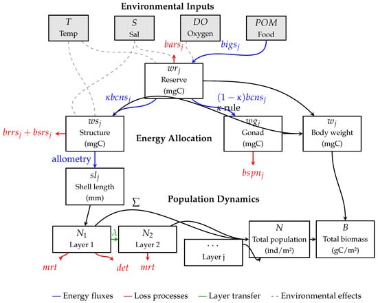
Figure 1.
Schematic representation of the DEB–statistical model for sessile organisms. Boxes represent state variables from the model equations (Table 1): (reserve materials), (structural materials), (gonadal materials), (shell length), (individual body weight), (population by layer), N (total population), and B (total biomass). Arrows represent processes and fluxes (Table 1): energy flows (blue), loss processes (red), layer transfers (green), and environmental effects (gray dashed).
At broader spatial scales, meta-population processes such as larval dispersal, connectivity among sites, and recruitment pulses can strongly influence local persistence under climate change. Our present model is explicitly single-site and does not include dispersal or source–sink dynamics. We therefore interpret results at the local population scale and acknowledge the absence of dispersal as a limitation (see Section 3.7).

Table 1.
Other equations implemented in the Sessile DEB–statistical model. Boxed equations indicate the key model outputs used to produce results (shell length, individual weight, population number, total biomass).
Table 1.
Other equations implemented in the Sessile DEB–statistical model. Boxed equations indicate the key model outputs used to produce results (shell length, individual weight, population number, total biomass).
| Variable | Equation |
|---|---|
| Temperature–filtration factor | |
| Temperature–respiration factor | |
| Salinity–filtration factor | |
| Salinity–respiration factor | |
| Oxygen solubility | |
| Dissolved oxygen saturation | |
| Dissolved oxygen limitation | |
| Seston | |
| Food carbon | |
| Respiration modifier 1 | |
| Assimilation efficiency | |
| Energy gain | |
| Energy loss | |
| Respiration modifier 2 | |
| Filtration rate | |
| Potential ingestion | |
| Maximum ingestion | |
| Actual ingestion | |
| Active respiration | |
| Routine respiration | |
| Standard respiration | |
| Consumption | |
| Spawning biomass |
2. Methods
Our model simulates the dynamics of sessile organisms using a modified dynamic energy budget (DEB) approach. The framework tracks individual organisms within a population, modeling their growth, energy allocation, reproduction, and responses to environmental conditions. The model operates at two scales: (1) individual bioenergetics and (2) population dynamics including detachment, competition for space, and layering.
The model consists of several interconnected modules (Figure 1). The core bioenergetic module follows the standard DEB theory [20], tracking energy flow through an organism. Energy from food is first assimilated and then allocated to maintenance, growth, and reproduction according to the kappa rule [21]. The environmental response module modifies these energy flows based on temperature, salinity, and dissolved oxygen conditions [22]. The detachment module and mortality module calculate probabilities of organism loss as functions of environmental conditions and organism state. Finally, the spatial competition module manages population density and layering dynamics when space becomes limited.
Specifically, in our model, mussels are divided into multiple groups based on the layering structure of the mussel bed. Let denote the total number of groups, with representing the surface (food-facing) layer, representing the inner living layers. The living biomass of mussels is then
where is the total biomass of mussels in group j, is the number of mussels in group j and is the mean body weight of a mussel in group j.
2.1. Bioenergetic Growth Submodel
In the bioenergetic growth submodel, the body weight of a mussel in group j is partitioned into reserved materials (, mgC), structural materials (, mgC), and gonadal materials (, mgC):
A mussel filters ambient suspended particles (organic and inorganic). A net fraction of organic matter is assimilated into reserves (after feces), while reserves are mobilized to fuel maintenance, growth, and reproduction. The discrete-time updates (time step , in days) follow
where
- -
- (mgC day−1): net ingestion flux to reserves (post-feces assimilation);
- -
- (mgC day−1): reserve mobilization (consumption) flux;
- -
- , , (mgC day−1): standard, routine, and active respiration costs, respectively;
- -
- (mgC day−1): spawning (gonad loss) flux;
- -
- (-): allocation fraction of mobilized reserves to structure/maintenance [23].
In DEB theory, the -rule specifies that a fixed fraction of mobilized reserve () is allocated to somatic maintenance and growth (structure), while the remaining fraction is available for maturation and reproduction. Maintenance has priority; when is insufficient to cover maintenance costs, growth ceases and reserves are used to meet maintenance before any allocation to reproduction occurs [12,21]. The modeling of each variable is summarized in Table 1.
Structural materials are closely linked to shell length. Using the same allometry as in the model summary (Table 1),
where denotes shell length (mm) for group j (i.e., ).
2.2. Mortality and Detachment Module
The model includes two distinct processes for population loss: mortality and detachment.
For mortality, we implemented an empirical equation developed by Ma et al. [24] from experimental studies on Asian green mussels (Perna viridis). Although the dominant species in our study was the blue mussel (Mytilus galloprovincialis), contributing over 99% of the biomass, this equation was adopted as a reasonable approximation. The justification lies in the physiological similarities between these two species from the Mytilidae family, which are known to exhibit comparable responses to environmental stressors such as temperature and salinity [7]:
where M is the mortality rate over a 7-day period, T is temperature and S is salinity. For other species or study systems, these parameters would need to be recalibrated to reflect species-specific physiological responses.
For the detachment component, we developed a physiological stress model based on the optimization of field-collected detachment data. The model uses logistic response curves [25] for both temperature and salinity stress, with a synergistic interaction term [26]:
where D is the detachment rate over a 20-day period, is temperature stress (increasing with temperature above ), is salinity stress (decreasing with salinity below ), and control the transition steepness of the stress responses, represents the strength of the synergistic interaction between stressors, is the baseline detachment rate under optimal conditions, and is the maximum detachment rate under extreme stress.
The optimized parameter values for our study system were °C, , psu, , , , and . These values were determined through gradient-based optimization (L-BFGS-B method) to minimize the mean squared error between predicted and observed detachment rates.
ANOVA was used to assess the performance of the nonlinear stress model. The total variability in detachment rates was partitioned into regression and error components, resulting in an F-statistic of 8.0417 and a p-value of 0.0317 (with 6 and 4 degrees of freedom for the model and error, respectively). This indicates that the model is significant. A lack-of-fit test was not performed due to the lack of replication. The optimal conditions for minimizing the detachment rate were then determined using a grid search method (see Section 3.2).
To convert the 20-day detachment rate to a daily rate, we must account for the cumulative nature of the detachment process. If we denote the daily detachment rate as , then the relationship between the 20-day detachment rate D and is given by
Solving the daily detachment rate requires
Similarly, the daily mortality rate is
2.3. Competition Submodel
The competition for space and food among mussels is modeled as a function of the population density of mussels. The growth of mussels leads to competition for space. Space limitation is handled explicitly via layer formation when the occupied area exceeds the available substrate. Let denote the available substrate area, the current number of layers, the number of individuals in layer j, and the representative shell length for layer j.
Individual area demand (per mussel) is given by
The total occupied area () and the overcapacity fraction are
Here, is the capacity area, i.e., the area of substrate attached by sessile organisms. The model assumes that space occupied by dead individuals becomes available for settlement immediately upon mortality. While a more complex model could certainly include a state variable for the area occupied by empty shells, we opted for this more parsimonious approach to limit the number of model parameters for which we have limited empirical data (e.g., shell decay rates).
When , a fraction of the outermost layer () population is transferred to the next layer:
This operator can cascade if overcapacity persists, resulting in additional layers. The total living population is
The population affected by detachment and mortality is
Here, t indexes the discrete daily step and n the within-step update.
To represent the mixing of physiological states caused by this transfer, for any per-capita state variable (shell length, reserves, structure, and gonad), the inner layer state after transfer is the weighted average
When , no transfer or mixing occurs.
Following transfer, inner layers (disadvantaged in food access) are assumed to enter a reserve-driven regime with no feeding, where reserves fuel standard maintenance and allocation. For layers ,
The outermost layer () remains food-facing and follows the full DEB dynamics with ingestion.
For a comprehensive overview of the model equations, please refer to Table 1.
2.4. Case Study
The model was applied to simulate sessile organism populations around a floating platform that moors the training ship Shioji-maru of Tokyo University of Marine Science and Technology in the estuary of the Sumida River, Japan (Figure 2). Field data were collected from September 2002 to September 2003. Artificial substrata including polyvinyl chloride plates (30 cm diameter) and acrylic plates (20 cm × 20 cm) were deployed to monitor biofouling dynamics. Environmental parameters including water temperature, salinity, dissolved oxygen, chlorophyll a, and turbidity were measured continuously using automated sensors (Table 2). The dominant sessile organism was the blue mussel Mytilus galloprovincialis, which formed dense multi-layered aggregations on seawalls and piles around the floating platform.
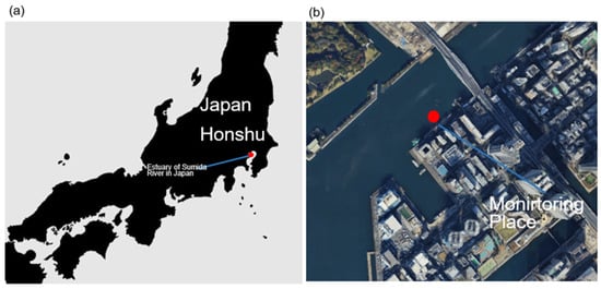
Figure 2.
Study location in the estuary of the Sumida River, Japan. (a) Map showing the location of the study site in the estuary of the Sumida River, Honshu, Japan. (b) Satellite image of the monitoring place, indicating the floating platform mooring the training ship Shioji-maru with the arrangement of monitoring equipment and artificial substrata for water quality measurement and multi-layer structure examination.
Table 2.
Summary of water quality monitoring instruments and setup.
The study site was characterized by estuarine conditions with variable environmental parameters driven by freshwater input from the Sumida River and tidal exchange with Tokyo Bay. Water quality sensors were positioned at 50 cm below the surface and maintained through regular cleaning every two weeks (weekly during summer) to prevent biofouling interference. Additional water quality data including particulate organic matter (POM) and particulate inorganic matter (PIM) concentrations were obtained from monitoring stations at Tsukuda Bridge and Reimei Bridge to provide comprehensive food availability estimates for the bioenergetic model.
To monitor population dynamics and physiological responses, multiple experimental approaches were employed. Artificial substrata suspended in nets allowed for regular sampling of mussel aggregations every two weeks, with detailed measurements of wet weight, shell length, and spatial distribution. Oxygen consumption rates were measured using bell jar experiments, where mussels and surrounding seawater were enclosed for 45 min while monitoring dissolved oxygen concentration changes. These physiological measurements provided critical validation data for the DEB model parameters.
The multi-layer structure analysis involved a systematic examination of mussel positioning within dense aggregations. Mussels were categorized into three distinct layers based on shell gape visibility from the surface: the first layer (gape completely exposed), second layer (gape partially exposed), and third layer (gape completely buried). This layering classification provided essential data for validating the spatial competition module of the model and understanding resource limitation effects in dense assemblages.
Sensor maintenance: every two weeks (every one week in summer) for cleaning and data transfer.
2.5. Computational Conditions
The model was implemented in Fortran 90 and ran with a primary time step of 1 day (86,400 s) for state updates, while certain internal fluxes are integrated at a finer internal resolution (seconds) to ensure numerical stability. The simulation period covered September 2002 through September 2003. Parameter values were initially derived from the literature sources (see Table 3) for blue mussels (Mytilus edulis and Mytilus galloprovincialis), as they are among the most extensively researched sessile organisms [27] and they are the dominant species in our case study (Table 3).
Table 3.
Physiological parameters used in the model.
The initial conditions were set based on observational data. The starting shell length (sl) for mussels was established at 5 mm, with an initial population density (pn) of 300,000 individuals per square meter. The initial structural material (ws) is calculated based on the shell length. The reserved material (wr) is defined as 10% of the structural material. As mussels with a 5 mm shell length are not yet mature, the initial gonadal material (wg) is assumed to be zero.
For each simulation, the model was initialized with empirically observed environmental conditions, initial organism densities and shell length. Environmental forcing variables (temperature, salinity, dissolved oxygen, and food concentration) were interpolated from field measurements to provide continuous inputs to the model.
3. Results and Discussion
3.1. Biomass Dynamics
The full simulation (Figure 3) incorporating both mortality and detachment mechanisms closely aligns with the observed biomass measurements throughout the study period. When comparing the different simulation scenarios, the contrast is striking; the simulation excluding both mortality and detachment (dotted line) predicts a biomass accumulation reaching approximately 1500 g by mid-2003, which is substantially higher than the observed values.
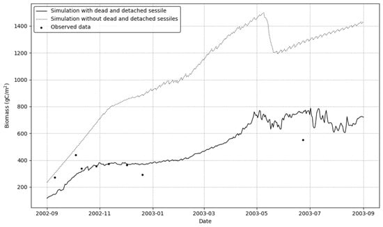
Figure 3.
Illustrationof comparative results of simulation model under different mechanistic scenarios alongside observed field data. The figure shows predicted biomass (gC/m2) under two simulation scenarios: full simulation with mortality and detachment (solid line) and simulation without mortality and detachment (dotted line). Black dots represent field measurements.
This dramatic difference highlights the critical importance of including mortality and detachment mechanisms in bioenergetic models. Under the environmental conditions experienced at the study site, these combined processes were the dominant mechanism controlling population size. The simulation without these regulatory processes shows unrealistically high biomass accumulation that does not match the field observations.
The close correspondence between our full simulation results and field observations validates the model’s capability to accurately capture the complex dynamics of sessile organism populations.
3.2. Detachment Dynamics
The instantaneous detachment weight (Figure 4a) shows significant variability. After a period of low detachment from September 2002 to April 2003, the rate began to increase, rising sharply from May 2003. It exhibited strong fluctuations from July to September 2003, with peaks reaching approximately 4 gC/m2/day.
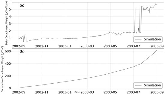
Figure 4.
Temporal dynamics of organism detachment under variable environmental conditions from September 2002 to September 2003. The simulation shows both instantaneous (a) and cumulative (b) detachment patterns throughout the monitoring period.
These temporal patterns in detachment dynamics coincided with seasonal changes in environmental parameters, particularly temperature and salinity. The increase in detachment from spring to summer 2003 aligns with rising water temperatures, which trigger physiological stress responses when they exceed optimal thermal ranges. The high variability in late summer suggests a complex interplay of environmental stressors during this period.
The cumulative detachment weight (Figure 4b) demonstrates a steady increase throughout the monitoring period, with the model simulation predicting a total cumulative detachment of approximately 600 gC/m2 by September 2003.
Our grid search optimization approach identified precise conditions for minimizing detachment, a temperature of 22.00 °C and salinity of 32‰, corresponding to a minimum detachment rate of . This finding aligns with previous physiological studies on bivalves [28,34] but provides a more specific quantification of optimal conditions. The systematic exploration of the temperature–salinity parameter space revealed a relatively narrow optimum window, with detachment rates increasing rapidly outside these conditions.
The model confirms that detachment responds non-linearly to environmental stressors, with synergistic effects between temperature and salinity as implemented in Equations (7)–(9) and (11). This mathematical relationship successfully reproduces the observed detachment patterns and supports the hypothesis that multiple stressors interact in ways that cannot be predicted by examining each factor in isolation.
The synergistic effect of temperature and salinity on marine invertebrates is a well-documented phenomenon [37]. High temperatures can exacerbate the physiological stress caused by low salinity, as organisms must expend more energy on osmoregulation, leaving fewer resources to maintain attachment strength [38]. Conversely, suboptimal salinity can lower an organism’s thermal tolerance limits. Our findings are consistent with studies on other bivalves, which have shown that interactive effects of multiple stressors are often more significant than their additive effects [39]. By quantifying this synergy, our model provides a more realistic depiction of the environmental pressures facing sessile organisms in dynamic estuarine environments.
3.3. Mortality Rate Analysis
Figure 5 illustrates the temporal dynamics of mortality rates at the study site from September 2002 to September 2003. The pattern reveals distinct seasonal trends. Mortality rates were high in September 2002 (around 53%) before decreasing to a low of approximately 41% in late October. From November 2002, the rate began a steep and steady climb, peaking at nearly 60% for a sustained period from January to March 2003. Following this peak, mortality rates declined through the spring, reaching a minimum of around 37% in late June. A second, highly variable period of increased mortality occurred from July to September 2003, with rates fluctuating between 41% and 56%.
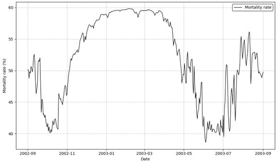
Figure 5.
Seasonal variation in mortality rates of sessile organisms from September 2002 to September 2003.
The periods of high mortality correspond to seasonal temperature extremes. The primary peak from January to March 2003 aligns with the coldest winter water temperatures, indicating that low temperatures were a major source of physiological stress. The decline in mortality from April to June corresponds with the transition to more favorable spring conditions. The second peak during the summer months of July and August aligns with high water temperatures, another period of thermal stress.
This bimodal pattern, with high mortality in both winter and summer, is consistent with the predictions from Equation (6), where the optimal temperature is 23.698 °C and the optimal salinity is 32‰. The model effectively captures how physiological stress is amplified at both low and high temperature extremes, likely interacting with salinity to drive mortality. The close correspondence between the simulated seasonal mortality trends and the model’s formulation validates its ability to capture the complex, non-linear responses of sessile organisms to environmental stressors.
3.4. Population Dynamics Analysis
The temporal evolution of the sessile organism population demonstrated a dramatic and continuous decline throughout the monitoring period (Figure 6). The simulation began in September 2002 with a very high population density of approximately 275,000 individuals/m2. This was followed by a steep and steady decrease, with the population density falling to around 100,000 individuals/m2 by January 2003 and further declining to below 25,000 individuals/m2 by the end of the study period in September 2003.
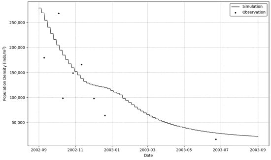
Figure 6.
Temporal dynamics of sessile organism population from September 2002 to September 2003. The continuous line represents simulation results, while black dots indicate field observations of population counts.
This substantial population crash aligns precisely with the high mortality rates detailed in Section 3.3. The sharp decline observed from autumn 2002 through the winter of 2003 directly corresponds to the period of extreme thermal stress where mortality rates peaked near 100%. The population continued to decline, albeit at a slower pace, through the summer of 2003 as organisms faced a second period of stress from high temperatures.
The validation of our numerical model against empirical observations demonstrates its efficacy in reproducing these harsh population dynamics. The close agreement between the simulated and observed population numbers throughout the year-long decline indicates that our approach effectively captures the mortality processes governing the sessile organism community under severe environmental stress.
3.5. Shell Length Analysis
Figure 7 illustrates the temporal evolution of shell length across different layers of sessile organisms and their final distribution by layer. The data reveal distinct patterns of growth and resource competition within the layered community structure.
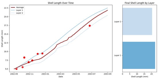
Figure 7.
Temporal dynamics and final distribution of shell length in layered sessile organisms. Left panel: Evolution of shell length (mm) across two layers from September 2002 to September 2003, showing simulation results (lines) and field observations (dots). Right panel: Final shell length distribution by layer.
An analysis of shell length dynamics over time demonstrates a clear stratification effect, with significant differences in growth trajectories between the outer (Layer 1) and inner (Layer 2) layers. The left panel shows that organisms in Layer 1 consistently grew faster and achieved a larger final size of approximately 22.5 mm. In contrast, organisms in Layer 2 experienced slower growth, reaching a final size of about 21 mm. The simulation results closely track the field observations throughout the study period, validating the model’s growth predictions.
The final shell length distribution, shown in the right panel, confirms this size disparity. The body size differences between the two layers follow a gradient that corresponds to resource availability. Organisms in Layer 1 achieved a larger final size, while those in Layer 2 exhibited smaller dimensions. This gradient reflects diminishing access to resources with increasing depth in the community structure.
These findings align with theoretical predictions from our spatial competition module (Equation (19)), which anticipated resource limitations in deeper layers. The model successfully captured the size gradients observed between the layers, demonstrating that competition for space—and consequently for food and oxygen—represents a fundamental structuring mechanism in sessile communities. Positioning relative to the water column serves as a primary determinant of growth potential and survival probability.
3.6. Individual Mean Weight Analysis
Figure 8 illustrates the temporal dynamics of average individual weight distribution across different layers of sessile organisms from September 2002 to September 2003. The data reveal distinctive patterns of biomass allocation and resource utilization within the layered community structure.
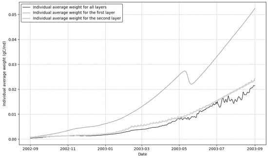
Figure 8.
Temporaldynamics of average wet weight distribution across community layers from September 2002 to September 2003. The black line represents the overall average wet weight across all layers, while light gray and dark gray lines show the average wet weight for the first and second layers, respectively.
The average weight for the first layer (the light gray line) consistently exceeded the others, showing steady growth to a peak of approximately 0.06 gC/ind and demonstrating the advantageous position of organisms with direct access to the water column. In contrast, the second layer (the dark gray line) exhibited much slower growth, reaching only about 0.025 gC/ind. The average weight for all layers combined (the black line) was the lowest and showed the most fluctuation, particularly after May 2003. A noticeable dip in the first layer’s growth occurred in May 2003 before it resumed an upward trend.
The data clearly illustrate that layer position strongly influences individual organism performance. The consistent and widening gap between the growth curves for the first and second layers highlights the critical importance of resource access in determining growth potential. This emphasizes how vertical positioning within the community structure serves as a primary determinant of biomass accumulation in sessile communities.
3.7. Limitation and Future Work
While our integrated DEB–statistical approach successfully modeled sessile organism dynamics, several limitations of the current study should be acknowledged and addressed in future research.
First, dispersal and meta-population connectivity are not represented. Recruitment from external sources and source–sink dynamics can buffer local populations against adverse conditions, especially under climate variability. Our single-site formulation therefore provides local-scale predictions and may underestimate persistence that would arise under strong connectivity among habitats.
A primary limitation of our approach is the reliance on literature-derived parameters predominantly calibrated for mussel species. In the present study, bivalves contributed over of biomass, making this approximation acceptable. However, applying this model to systems with multiple co-dominant sessile species would require significant additional parameterization efforts. Future work should focus on expanding the parameter database for non-bivalve sessile organisms and developing methods for integrating multiple species-specific DEB models within a single simulation framework.
The DEB-based model requires initial body length as a fundamental input parameter. We used a measured initial length of 5 mm as our initial condition. For studies with multiple co-dominant species, a more robust approach would incorporate weighted averages of body lengths across different species when such data are available. Future iterations of the model could implement dynamic initialization based on community composition surveys, allowing for a more accurate representation of mixed-species assemblages during the early colonization phase.
The current model framework is optimized for bivalves, particularly mussels, which dominated our study site. However, this approach overlooks the numerical significance of other sessile taxa in many field studies around the world. Future model development should incorporate parallel calculations for each taxonomic group, integrating results according to their relative contribution. This would enable a more comprehensive prediction of both weight dynamics and population structure, essential for understanding biodiversity patterns in sessile communities.
Finally, observational coverage is sparse beyond six months, with only one data point available after this period. This limits our ability to validate long-term dynamics and may increase uncertainty in late-stage predictions. Additional monitoring at longer durations would improve parameter identifiability and validation of the tail of the trajectories.
4. Conclusions
This study presents a comprehensive numerical framework that successfully integrates bioenergetic processes with environmental stress responses to predict sessile organism dynamics. Our combined DEB–statistical approach effectively captured complex patterns of growth, mortality, and detachment observed in the field, providing valuable insights into the mechanistic underpinnings of population fluctuations in sessile communities.
The model demonstrated that mortality and detachment respond to different environmental triggers, with mortality primarily controlled by sustained temperature extremes, while detachment exhibited greater sensitivity to synergistic interactions between temperature and salinity fluctuations. Our findings identified precise environmental thresholds (an optimal temperature of 22.00 °C and salinity of 32‰) that minimize detachment risk, providing quantitative targets for habitat management and aquaculture operations.
The layering dynamics revealed by our model highlight the critical importance of spatial positioning within sessile communities.
Importantly, the analysis of detachment dynamics offers further insight into the effects of benthic environmental variability, revealing how episodic stress events and resource limitations can drive community structure and turnover in sessile populations, establishing priorities for future research on benthic ecosystem modeling.
From an applied perspective, this modeling framework offers a valuable tool for predicting sessile organism responses to environmental variability, with particular relevance to aquaculture operations, biofouling management, and marine infrastructure planning. The demonstrated ability to accurately forecast biomass development and detachment events under variable conditions provides a quantitative basis for anticipating climate change impacts on coastal ecosystems.
Future research should focus on expanding this framework to incorporate species-specific parameterization, and broader taxonomic diversity. Integrating additional biological processes, such as reproduction and larval supply dynamics, would further enhance the model’s predictive capacity. As coastal environments face increasing pressures from climate change and anthropogenic activities, robust predictive models like the one presented here will become increasingly valuable for managing and conserving these ecologically and economically important communities.
Author Contributions
Conceptualization, T.T. and D.K.; methodology, T.T.; software, T.T.; validation, T.T.; formal analysis, T.T.; investigation, T.T.; resources, D.K., A.T., Y.Y. and M.H.; data curation, T.T.; writing—original draft preparation, T.T.; writing—review and editing, T.T., D.K., J.Z., A.T., Y.Y. and M.H.; visualization, T.T.; supervision, D.K.; project administration, D.K., Y.Y. and M.H. All authors have read and agreed to the published version of the manuscript.
Funding
This research received no external funding.
Data Availability Statement
All data included in this study are available upon request by contact with the corresponding author.
Acknowledgments
The authors would like to express their gratitude to National Institute for Environmental Research, Japan, for providing data of water quality in the estuary of the Sumida River.
Conflicts of Interest
The authors Akane Takahashi, Yoshinobu Yoneyama, Masanobu Hasebe are employed by the company Shimizu Corporation. The remaining authors declare that the research was conducted in the absence of any commercial or financial relationships that could be construed as a potential conflict of interest.
References
- Gili, J.M.; Coma, R. Benthic Suspension Feeders: Their Paramount Role in Littoral Marine Food Webs. Trends Ecol. Evol. 1998, 13, 316–321. [Google Scholar] [CrossRef]
- Gutiérrez, J.L.; Jones, C.G.; Strayer, D.L.; Iribarne, O.O. Mollusks as Ecosystem Engineers: The Role of Shell Production in Aquatic Habitats. Oikos 2003, 101, 79–90. [Google Scholar] [CrossRef]
- Venter, O.; Pillay, D.; Prayag, K. Water Filtration by Burrowing Sandprawns Provides Novel Insights on Endobenthic Engineering and Solutions for Eutrophication. Sci. Rep. 2020, 10, 1913. [Google Scholar] [CrossRef] [PubMed]
- FAO. The State of World Fisheries and Aquaculture 2022; FAO: Rome, Italy, 2022. [Google Scholar]
- Helmuth, B.; Mieszkowska, N.; Moore, P.; Hawkins, S.J. Living on the Edge of Two Changing Worlds: Forecasting the Responses of Rocky Intertidal Ecosystems to Climate Change. Annu. Rev. Ecol. Evol. Syst. 2006, 37, 373–404. [Google Scholar] [CrossRef]
- Miller, N.A.; Chen, X.; Stillman, J.H. Metabolic Physiology of the Invasive Clam, Potamocorbula amurensis: The Interactive Role of Temperature, Salinity, and Food Availability. PLoS ONE 2014, 9, e91064. [Google Scholar] [CrossRef]
- Fly, E.K.; Hilbish, T.J. Physiological Energetics and Biogeographic Range Limits of Three Congeneric Mussel Species. Oecologia 2013, 172, 35–46. [Google Scholar] [CrossRef]
- Petes, L.E.; Menge, B.A.; Murphy, G.D. Environmental Stress Decreases Survival, Growth, and Reproduction in New Zealand Mussels. J. Exp. Mar. Biol. Ecol. 2007, 351, 83–91. [Google Scholar] [CrossRef]
- Harley, C.D.G.; Randall Hughes, A.; Hultgren, K.M.; Miner, B.G.; Sorte, C.J.B.; Thornber, C.S.; Rodriguez, L.F.; Tomanek, L.; Williams, S.L. The Impacts of Climate Change in Coastal Marine Systems. Ecol. Lett. 2006, 9, 228–241. [Google Scholar] [CrossRef]
- Jackson, J.B.C. Competition on Marine Hard Substrata: The Adaptive Significance of Solitary and Colonial Strategies. Am. Nat. 1977, 111, 743–767. [Google Scholar] [CrossRef]
- Sebens, K.P. The Limits to Indeterminate Growth: An Optimal Size Model Applied to Passive Suspension Feeders. Ecology 1982, 63, 209–222. [Google Scholar] [CrossRef]
- Kooijman, B. Dynamic Energy Budget Theory for Metabolic Organisation, 3rd ed.; Cambridge University Press: Cambridge, UK, 2009. [Google Scholar]
- Sokolova, I.M.; Frederich, M.; Bagwe, R.; Lannig, G.; Sukhotin, A.A. Energy Homeostasis as an Integrative Tool for Assessing Limits of Environmental Stress Tolerance in Aquatic Invertebrates. Mar. Environ. Res. 2012, 79, 1–15. [Google Scholar] [CrossRef]
- Van Haren, R.J.F.; Kooijman, S.A.L.M. Application of a Dynamic Energy Budget Model to Mytilus edulis (L.). Neth. J. Sea Res. 1993, 31, 119–133. [Google Scholar] [CrossRef]
- Sarà, G.; Rinaldi, A.; Montalto, V. Trait-Based Bioenergetic Mechanistic Approach for Predictions of Life History Traits in Marine Organisms. Mar. Ecol. 2014, 35, 506–515. [Google Scholar] [CrossRef]
- Capelle, J.J.; Hartog, E.; Wilkes, T.; Bouma, T.J. Seasonal Variation in Cooperative and Competitive Behavior in Blue Mussels. PLoS ONE 2023, 18, e0293142. [Google Scholar] [CrossRef] [PubMed]
- Zardi, G.; McQuaid, C.; Nicastro, K. Seasonality of Wave Action, Attachment Strength and Reproductive Output in Mussels. Mar. Ecol. Prog. Ser. 2007, 334, 155–163. [Google Scholar] [CrossRef]
- Montalto, V.; Sarà, G.; Ruti, P.M.; Dell’Aquila, A.; Helmuth, B. Temporal Data Resolution and Predictions of Climate Change Effects on Bivalves. Ecol. Model. 2014, 278, 18150–18155. [Google Scholar] [CrossRef]
- Saurel, C.; Gascoigne, J.C.; Palmer, M.R.; Kaiser, M.J. In Situ Mussel Feeding Behavior. Limnol. Oceanogr. 2007, 52, 1919–1929. [Google Scholar] [CrossRef]
- Kooijman, S.A.L.M. Dynamic Energy Budgets in Biological Systems: Theory and Applications in Ecotoxicology; Cambridge University Press: Cambridge, UK, 1993. [Google Scholar]
- Nisbet, R.M.; Muller, E.B.; Lika, K.; Kooijman, S.A.L.M. From Molecules to Ecosystems through DEB Models. J. Anim. Ecol. 2000, 69, 913–926. [Google Scholar] [CrossRef]
- Baretta, J.; Ruardij, P. Tidal Flat Estuaries: Simulation and Analysis of the EMS Estuary; Springer: Berlin/Heidelberg, Germany, 1988. [Google Scholar]
- Bayne, B.L.; Gabbott, P.A.; Widdows, J. Some Effects of Stress in the Adult on the Eggs and Larvae of Mytilus edulis L. J. Mar. Biol. Assoc. UK 1975, 55, 675–689. [Google Scholar] [CrossRef]
- Ma, Z.; Fu, Z.; Yang, J.; Yu, G. Combined Effects of Temperature and Salinity on Perna viridis. Antioxidants 2022, 11, 2009. [Google Scholar] [CrossRef]
- Deutsch, C.A.; Tewksbury, J.J.; Huey, R.B.; Sheldon, K.S.; Ghalambor, C.K.; Haak, D.C.; Martin, P.R. Impacts of Climate Warming on Terrestrial Ectotherms across Latitude. Proc. Natl. Acad. Sci. USA 2008, 105, 6668–6672. [Google Scholar] [CrossRef]
- Côté, I.M.; Darling, E.S.; Brown, C.J. Interactions among Ecosystem Stressors. Proc. R. Soc. B 2016, 283, 20152592. [Google Scholar] [CrossRef]
- Bandara, N.; Zeng, H.; Wu, J. Marine Mussel Adhesion: Biochemistry, Mechanisms, and Biomimetics. J. Adhes. Sci. Technol. 2013, 27, 2139–2162. [Google Scholar] [CrossRef]
- Schulte, E.H. Influence of Algal Concentration and Temperature on Filtration Rate of Mytilus edulis. Mar. Biol. 1975, 30, 331–341. [Google Scholar] [CrossRef]
- Babarro, J.M.F.; Fernández-Reiriz, M.J.; Labarta, U. Growth of seed mussel (Mytilus galloprovincialis LMK): Effects of environmental parameters and seed origin. J. Shellfish Res. 2000, 19, 187–193. [Google Scholar]
- Widdows, J.; Fieth, P.; Worrall, C.M. Seston, Available Food and Feeding Activity in Mytilus edulis. Mar. Biol. 1979, 50, 195–207. [Google Scholar] [CrossRef]
- Clausen, I.; Riisgård, H.U. Growth, filtration and respiration in the mussel Mytilus edulis. Mar. Ecol. Prog. Ser. 1996, 141, 37–45. [Google Scholar] [CrossRef]
- Bayne, B.L.; Hawkins, A.J.S.; Navarro, E.; Iglesias, J.I.P. Effects of seston concentration on feeding, digestion and growth in the mussel Mytilus edulis. Mar. Ecol. Prog. Ser. 1989, 55, 47–54. [Google Scholar] [CrossRef]
- Tabeta, S.; Kinoshita, T.; Kitazawa, D.; Fujino, M.; Kato, T.; Sasaki, K.; Iume, T. Investigation for modelling of sessile organisms on coastal floating structures. In Proceedings of the ASME 2004 23rd International Conference on Offshore Mechanics and Arctic Engineering, Vancouver, BC, Canada, 20–25 June 2004. [Google Scholar] [CrossRef]
- Jørgensen, C.B.; Larsen, P.S.; Riisgård, H.U. Effects of Temperature on the Mussel Pump. Mar. Ecol. Prog. Ser. 1990, 64, 89–97. [Google Scholar] [CrossRef]
- Villalba, A. Gametogenic cycle of cultured mussel, Mytilus galloprovincialis, in the bays of Galicia (N.W. Spain). Aquaculture 1995, 130, 269–277. [Google Scholar] [CrossRef]
- Bayne, B.L.; Thompson, R.J. Some Physiological Consequences of Keeping Mytilus edulis in the Laboratory. Helgol. Mar. Res. 1970, 20, 526–552. [Google Scholar] [CrossRef]
- Delorme, N.J.; Sewell, M.A. Temperature and Salinity: Two Climate Change Stressors Affecting Early Development of the New Zealand Sea Urchin Evechinus chloroticus. Mar. Biol. 2014, 161, 1999–2009. [Google Scholar] [CrossRef]
- Jones, H.R.; Johnson, K.M.; Kelly, M.W. Synergistic Effects of Temperature and Salinity on the Gene Expression and Physiology of Crassostrea virginica. Integr. Comp. Biol. 2019, 59, 306–319. [Google Scholar] [CrossRef]
- Krishna, S.; Lemmen, C.; Örey, S.; Rehren, J.; Di Pane, J.; Mathis, M.; Püts, M.; Hokamp, S.; Kesari Pradhan, H.; Hasenbein, M.; et al. Interactive Effects of Multiple Stressors in Coastal Ecosystems. Front. Mar. Sci. 2025, 11, 1481734. [Google Scholar] [CrossRef]
Disclaimer/Publisher’s Note: The statements, opinions and data contained in all publications are solely those of the individual author(s) and contributor(s) and not of MDPI and/or the editor(s). MDPI and/or the editor(s) disclaim responsibility for any injury to people or property resulting from any ideas, methods, instructions or products referred to in the content. |
© 2025 by the authors. Licensee MDPI, Basel, Switzerland. This article is an open access article distributed under the terms and conditions of the Creative Commons Attribution (CC BY) license (https://creativecommons.org/licenses/by/4.0/).