
Automated Deployment of an Underwater Tether Equipped with a Compliant Buoy–Ballast System for Remotely Operated Vehicle Intervention


Abstract
1. Introduction
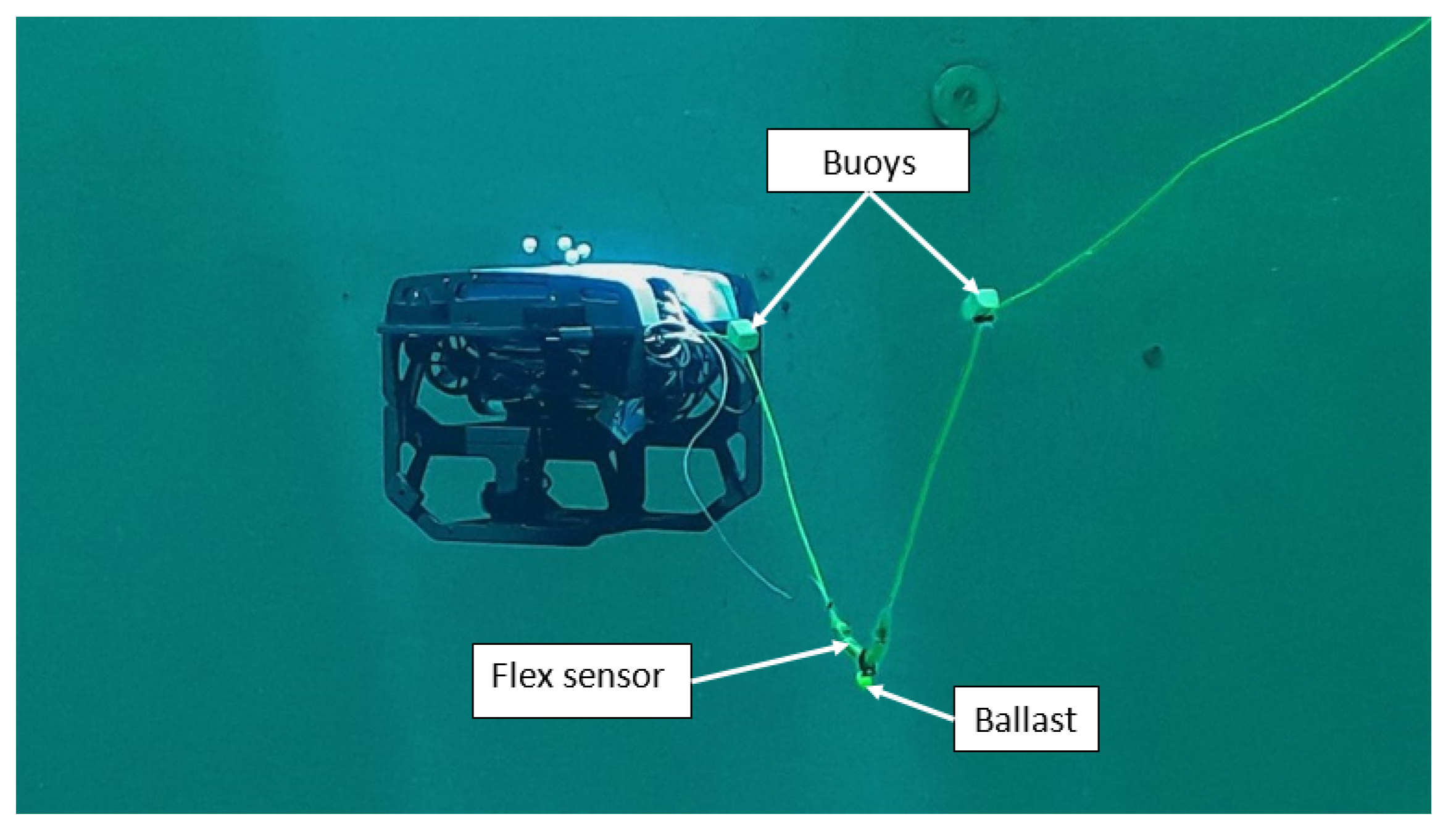
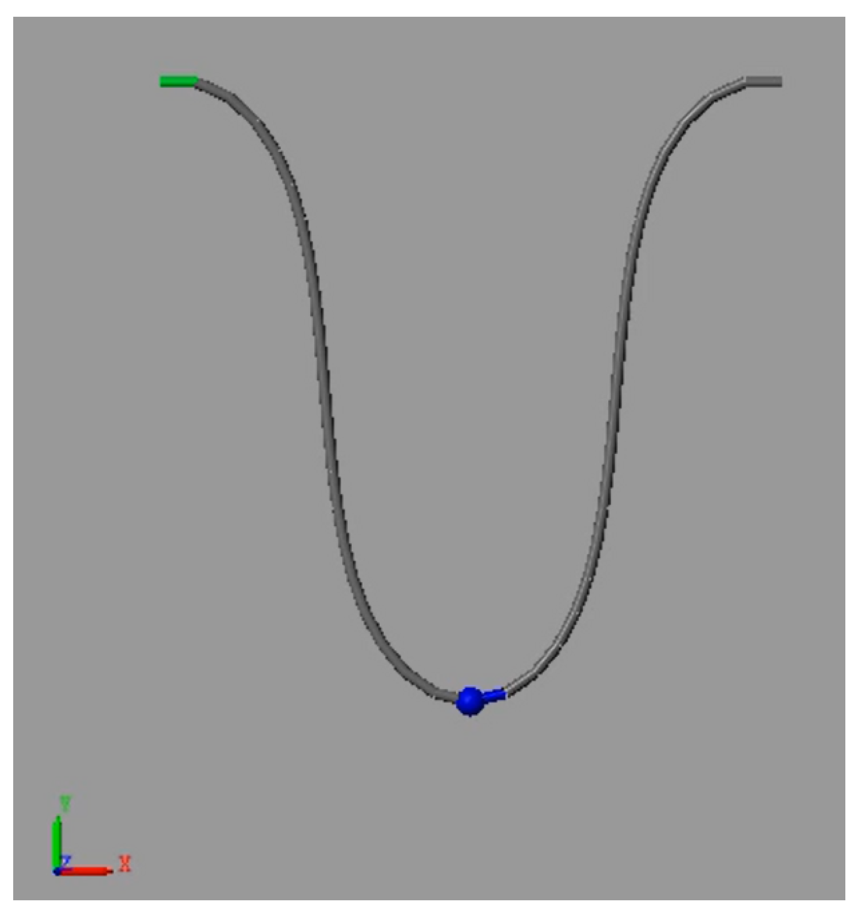
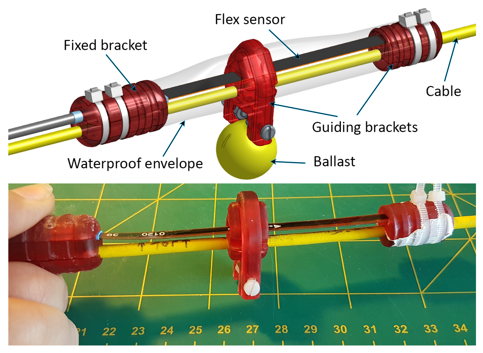
- The modeling, design, and implementation of the compliant-actuated system to equip the tether, which is composed of two symmetric buoys, one ballast, and one flex sensor located at the ballast;
- Tether length control by the feeder system on the surface, used to maintain the tether in a semi-stretched shape according to flex sensor feedback from the ROV;
- Simulations and real experiments to validate the solution by employing a compact underwater vehicle and a neutrally buoyant tether.
2. Modeling of The Compliant Buoy–Ballast Sensing System
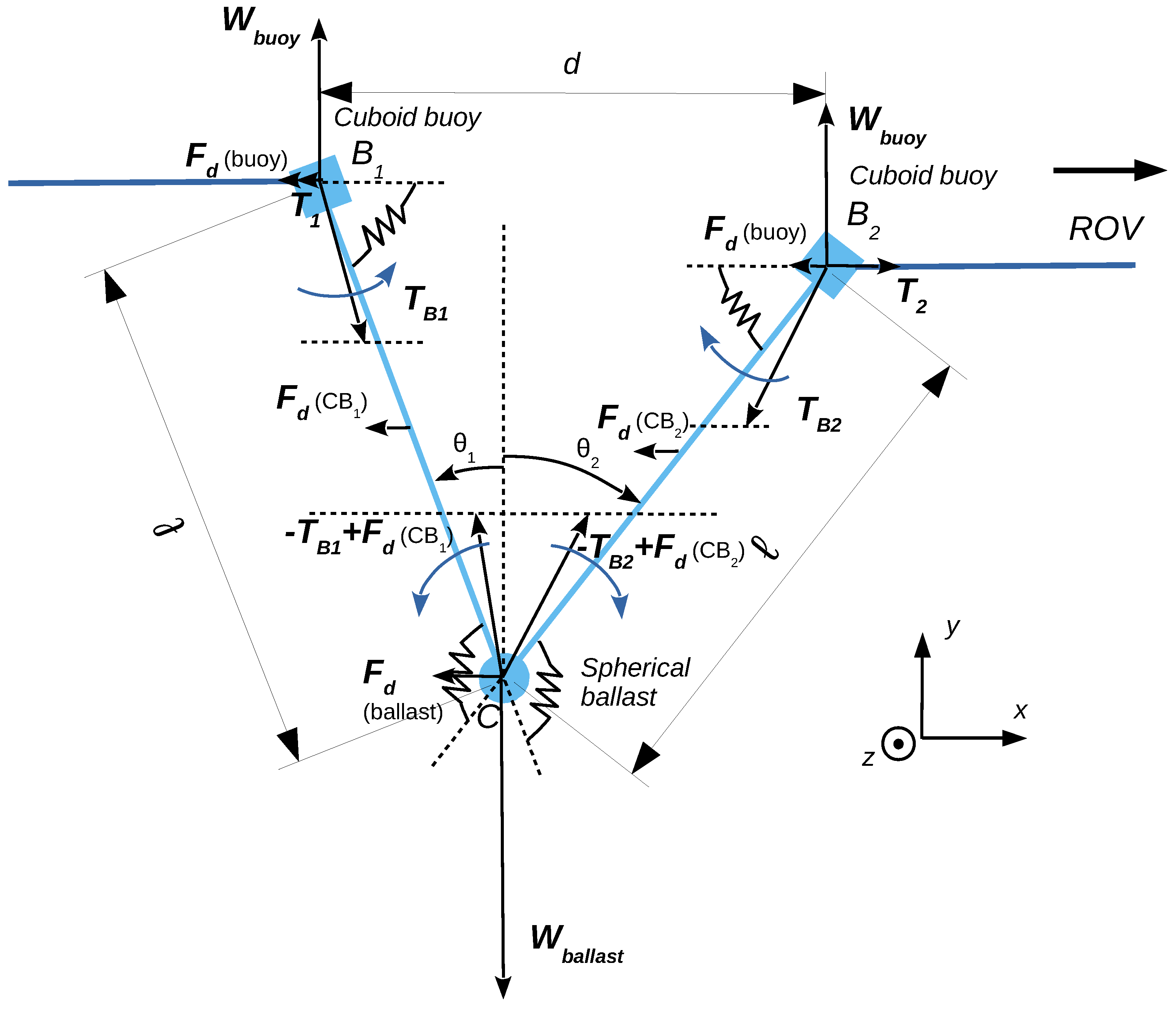
2.1. Neutral Buoyancy of The Buoy–Ballast System
2.2. Drag Forces
- k is a coefficient that depends on the shape of the object. For a sphere of radius R, .
- is the dimensionless quadratic drag coefficient, which is a property of the object. For a spherical shape, , and for a cuboid shape, .
- A is the cross-sectional area of the object, perpendicularly to the motion, which can be approximated by , with .
2.3. Distance Versus Speed in Steady-State Mode
- and are the components of the force that is exerted by the cable portion of length ℓ onto the left buoy.
- and are the components of the force that is exerted by the cable portion of length ℓ onto the right buoy.
- is the intensity of the drag force exerted by the fluid on the buoy.
- is the intensity of the drag force exerted by the fluid on the ballast.
- and are, respectively, the intensity of the drag force exerted by the fluid on the cable portion and .
- is the bending stiffness coefficient of the cable.
- and are, resp., the vertical angle of the cable portion and the cable portion.
- is the magnitude of the horizontal scalar force exerted by the cable that links the left buoy to the remote station.
- is the horizontal scalar force exerted by the cable that links the right buoy to the ROV. In the case of the figure, the intensity is positive since the ROV pulls on the cable to move from left to right.
2.4. Dynamics Analysis through Differential Equations
- for a laminar water flow.
- for a turbulent water flow.
2.5. Conclusions on the Use of Modeling
3. Simulations
- The numerical modeling of the V-shape system with Matlab–Simulink™ for precise sizing of the parameters ℓ and .
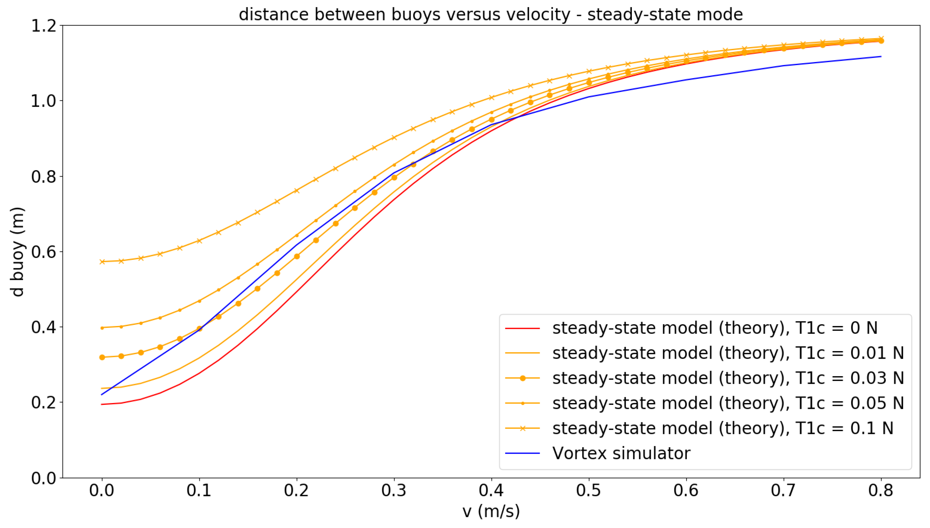
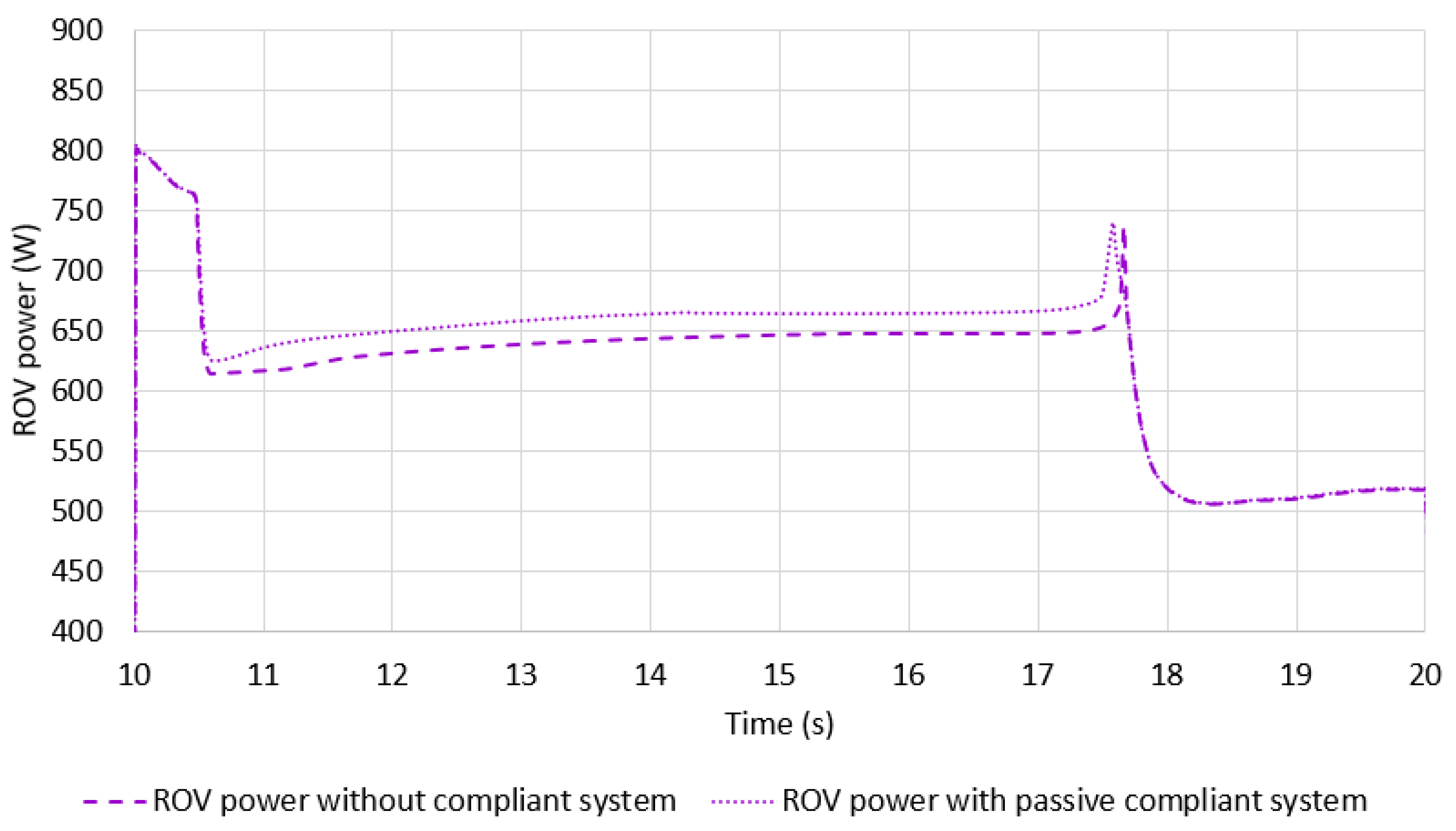
- A series of simulations run with the Vortex® simulator to check the validity of the V-shape system. In particular, the variation in the distance between buoys as a function of speed is observed and compared with the variation obtained using the theoretical model to check the steady-state mode. The influence of the V-shape system in terms of power consumption of the ROV is also evaluated. Then, a complete trajectory with varying depth, turns, and speed is simulated to observe the behavior of the V-shape system.
3.1. Numerical Modeling for Precise Sizing
3.2. Configuration for the Simulator
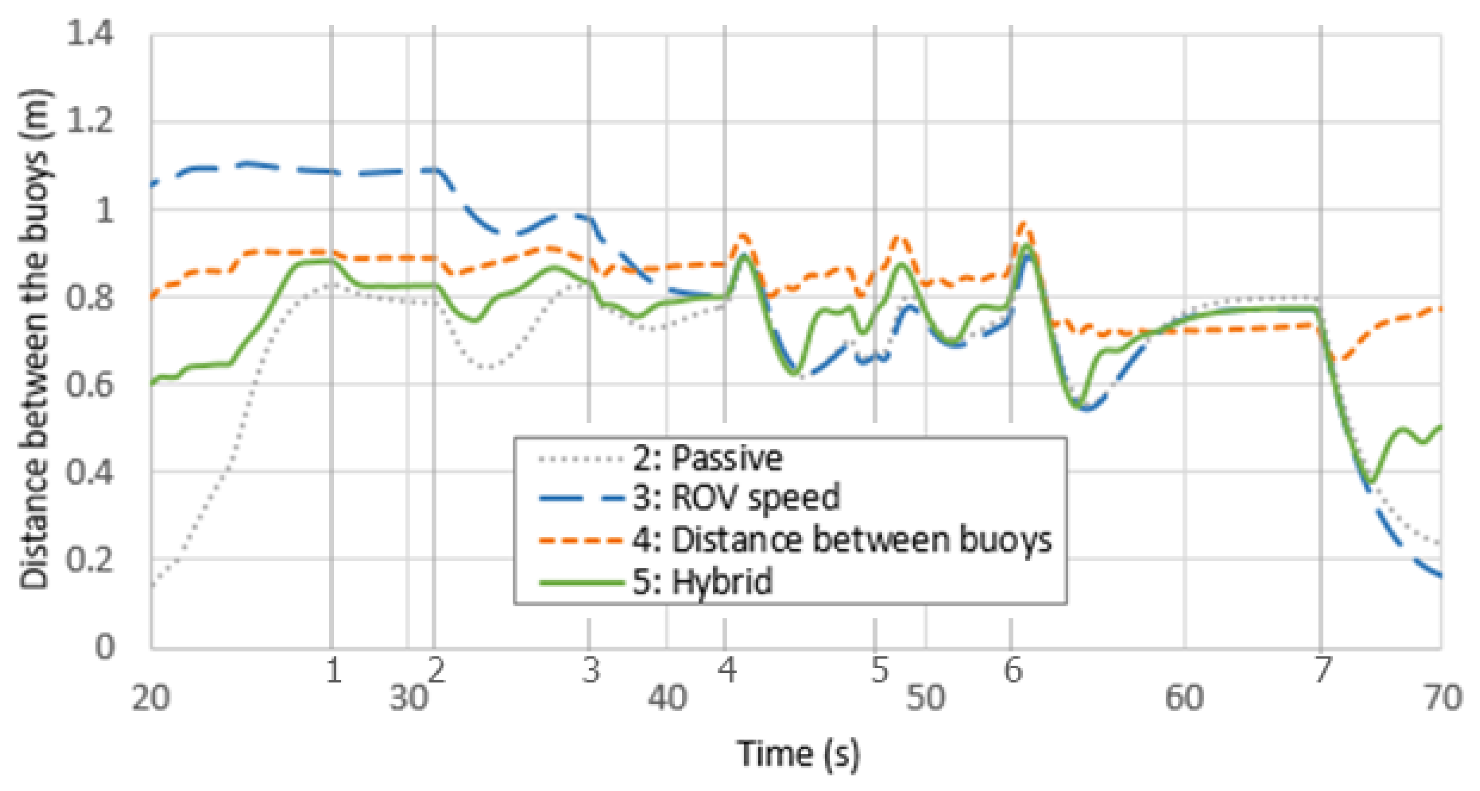
3.3. Study of the Distance between Buoys
3.4. Influence of Buoy–Ballast System on ROV Power
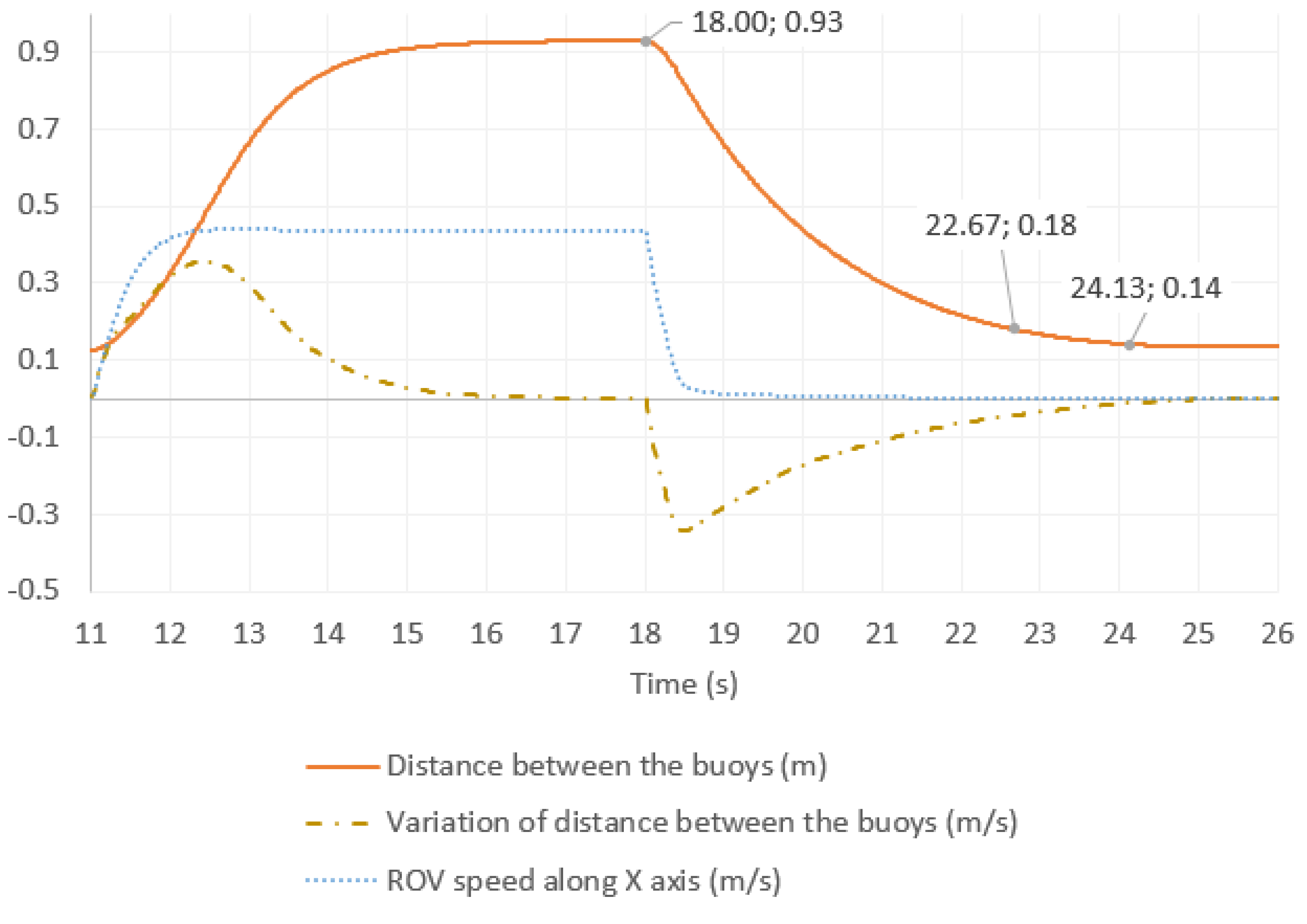
3.5. Generation of ROV Trajectories for Further Analysis
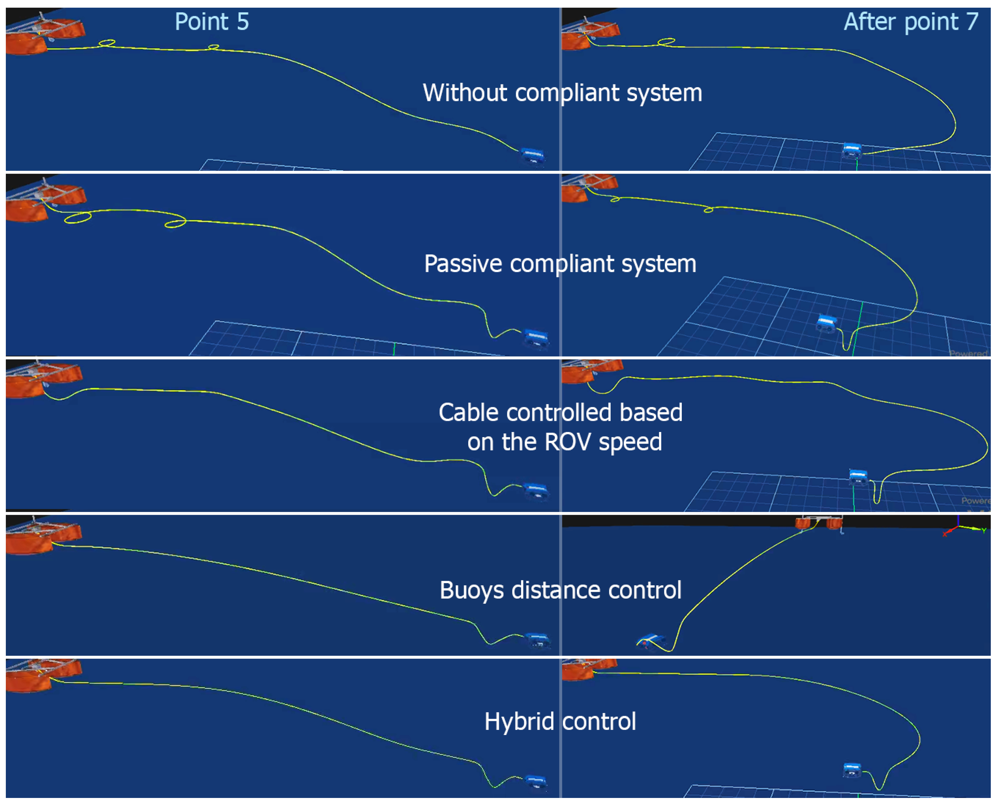
- Cable not controlled and without compliant system: the cable length is fixed to 15 m along the simulation.
- Cable with passive compliant system (not controlled): the cable length is fixed to 15 m along the simulation.
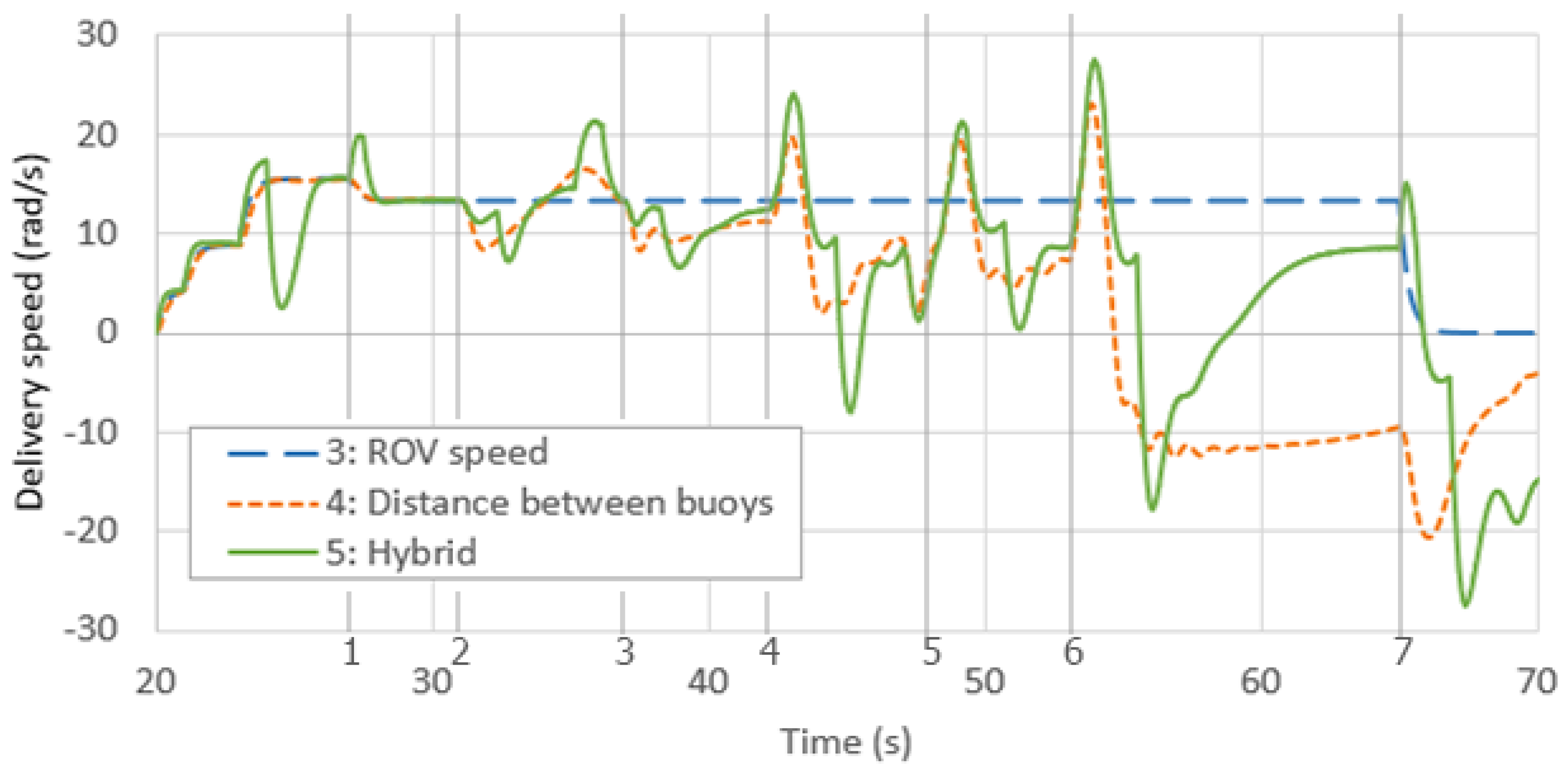
- Cable controlled with ROV speed command as input: the delivery speed of the cable is set to the ROV speed.
- Cable controlled with distance between the buoys: a closed-loop PD controller maintains a target distance of 0.8 m between the buoys.
- Hybrid control of the cable based on ROV speed and distance between buoys, which combines buoy distance PD controller and P controller using an ROV speed command. Furthermore, the target distance between the buoys is set to vary according to the ROV speed. The proportional part of the PD controller on the buoys’ distance works only if the distance is at least 5 cm longer than the target (taut cable) or if it is less than the target for more than 1 s (slack cable).
- Of the three controllers evaluated in the simulation, the ROV speed-based controller is not sufficiently responsive and generates a static error on the buoys’ distance that is never corrected. It is therefore not robust to external disturbances.
- The control mode based on the distance between buoys is rather smooth, robust, and reactive.
- The hybrid control is quite reactive but presents some more pronounced oscillations while remaining rather stable. Hybrid control could possibly be improved by replacing the ROV command speed with the actual ROV speed, which would require the use of more sensors on the ROV, such as a Doppler velocity log (DVL).
4. Description of Setup, Control Mode, and ROV Trajectories for Real Experiments
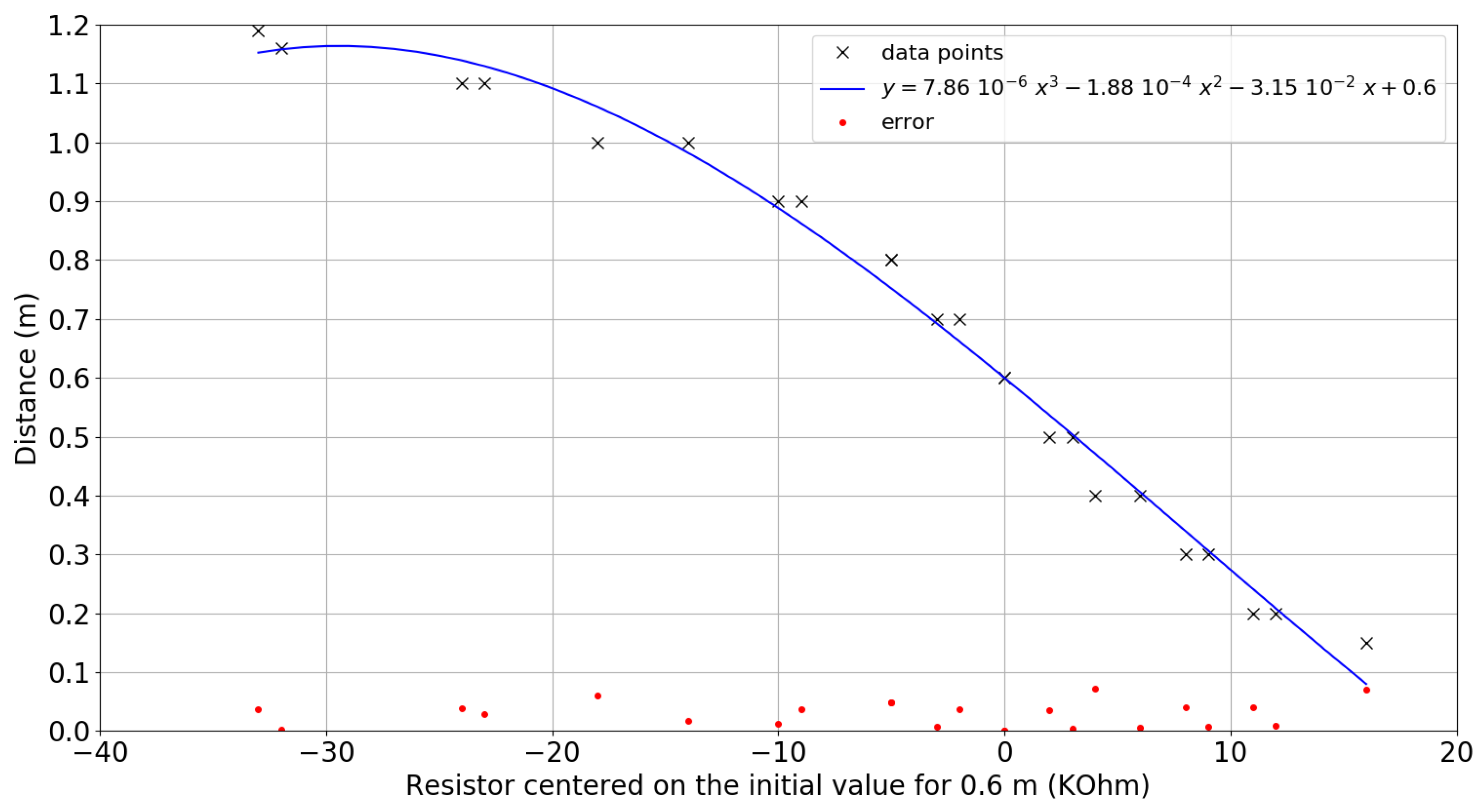
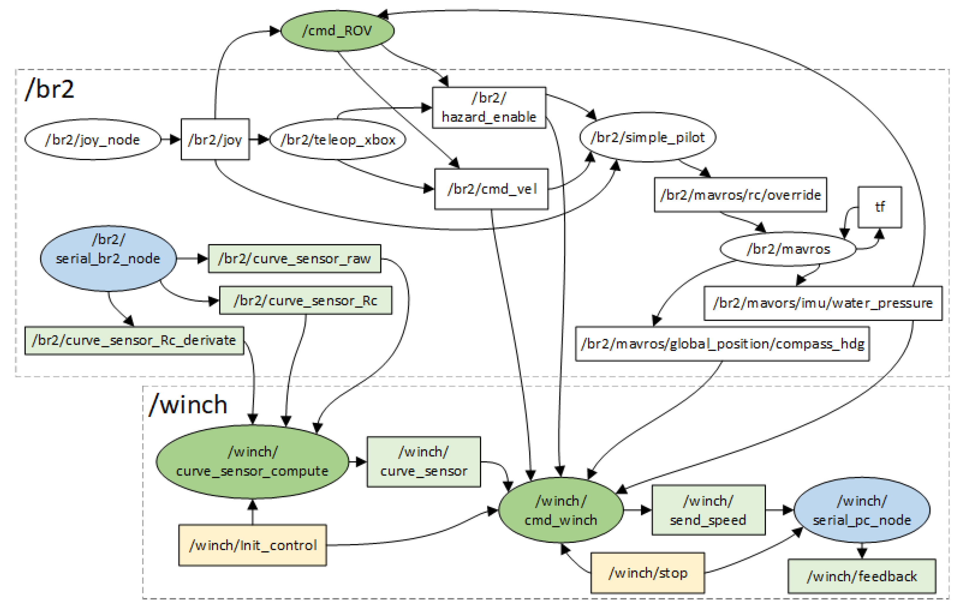
4.1. Setup
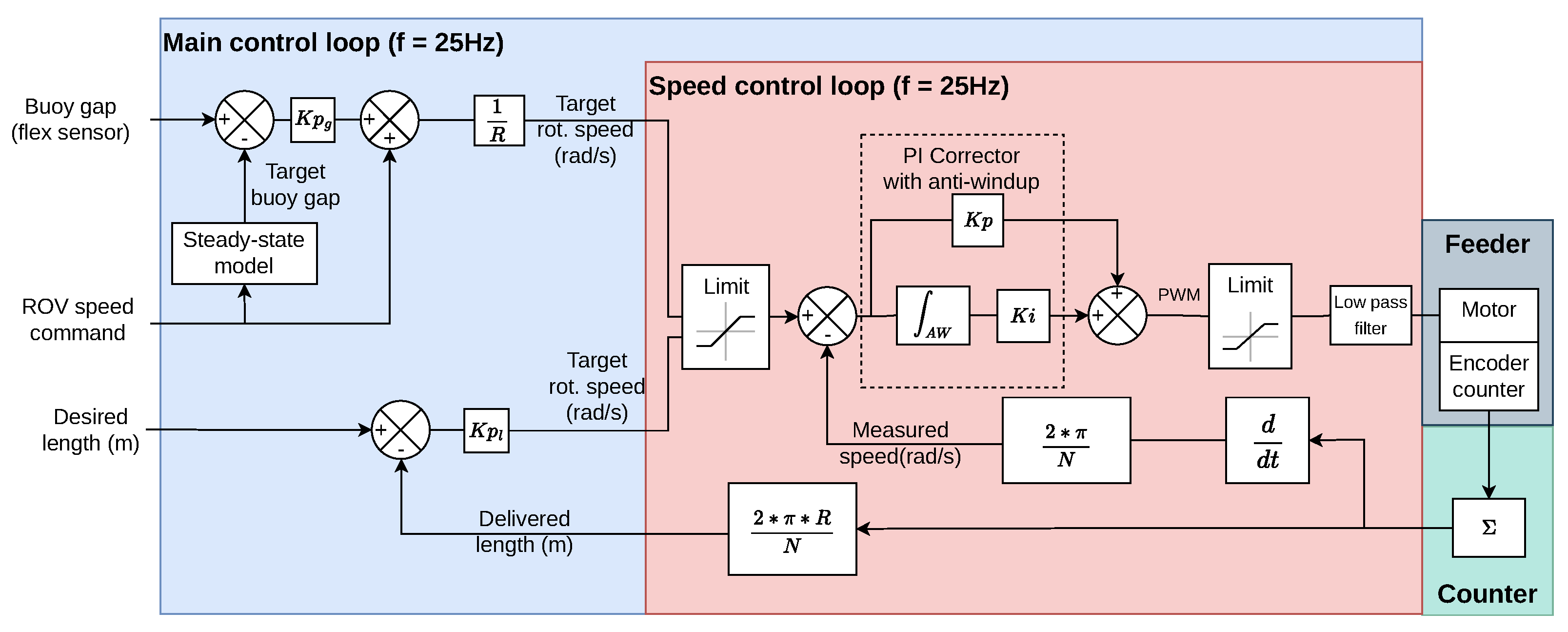
4.2. Control Scheme
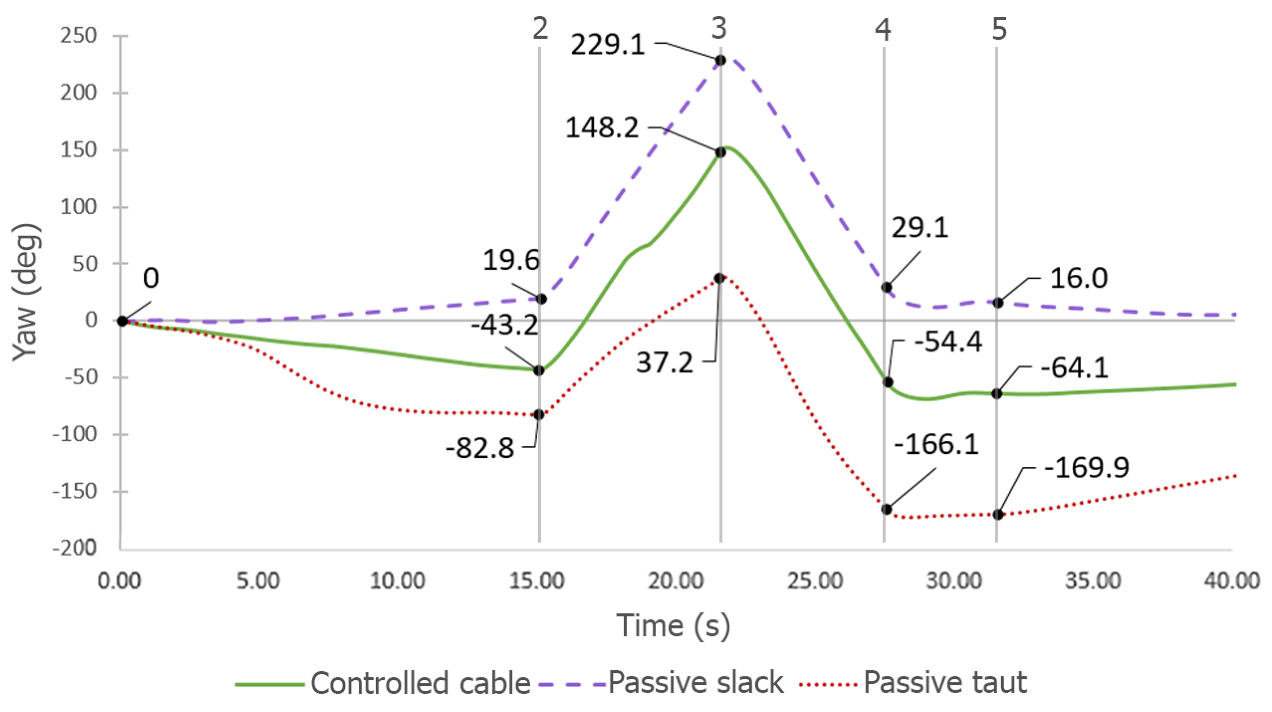
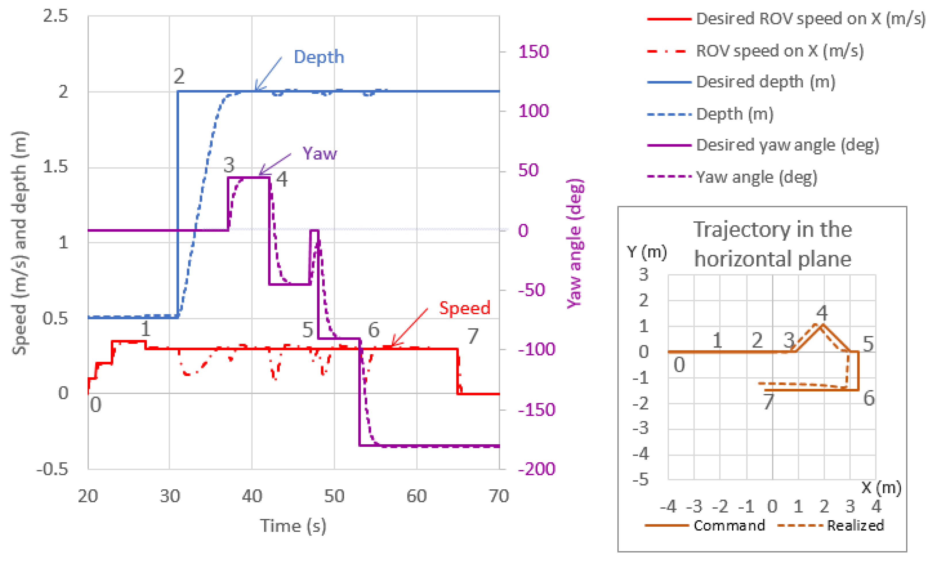
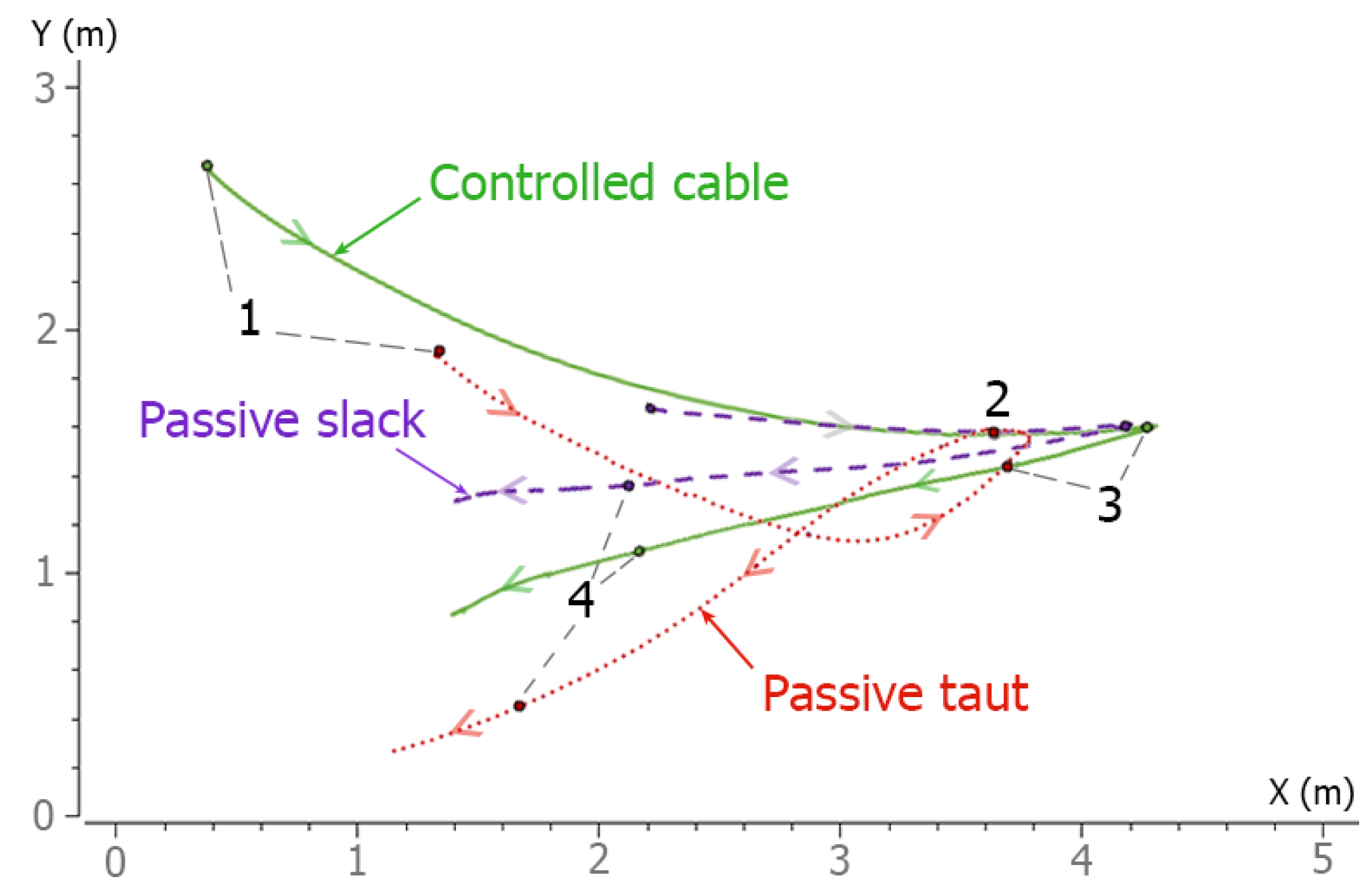
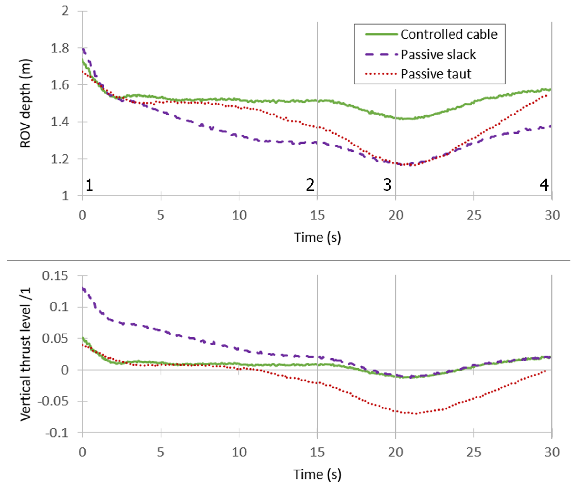
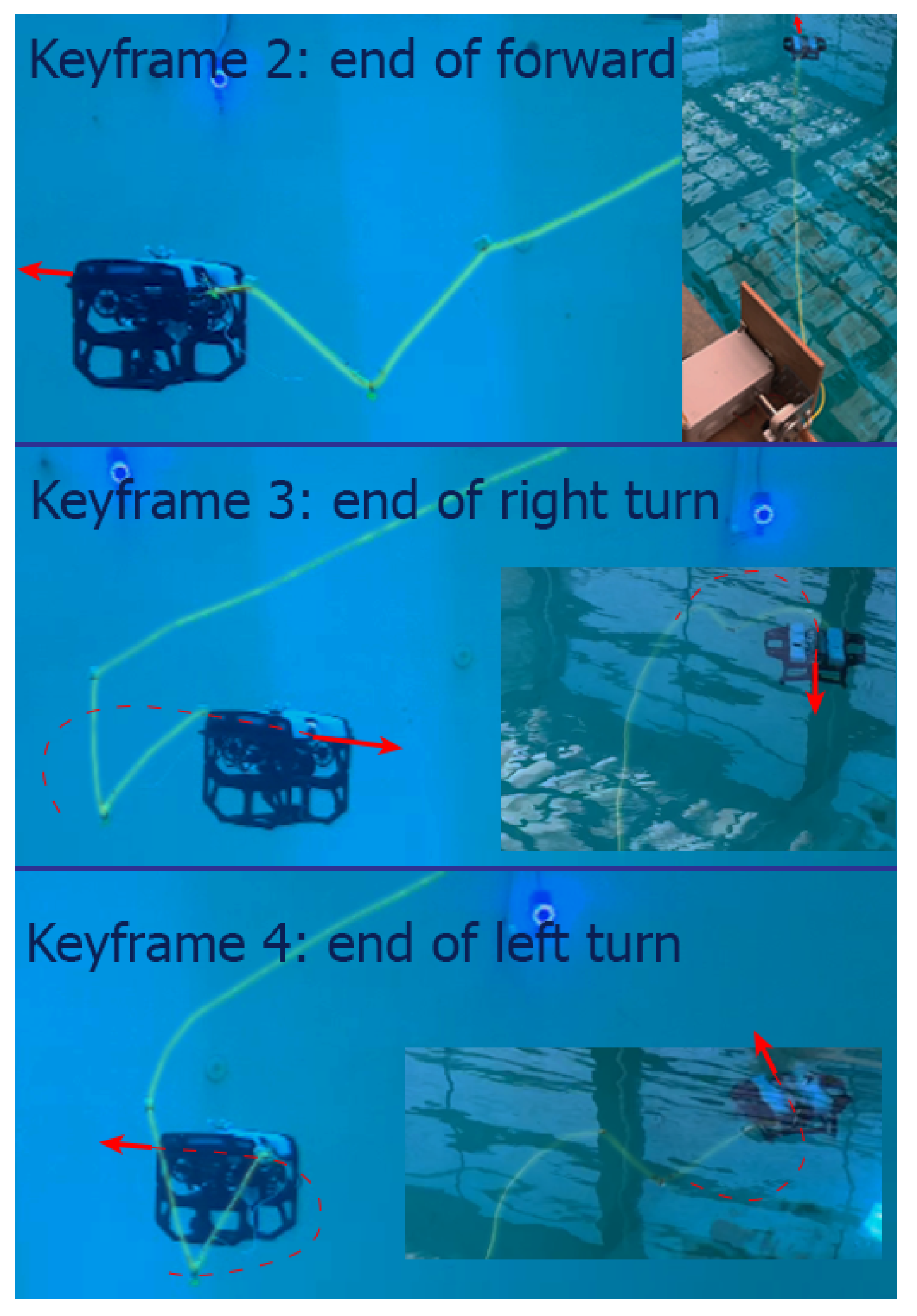
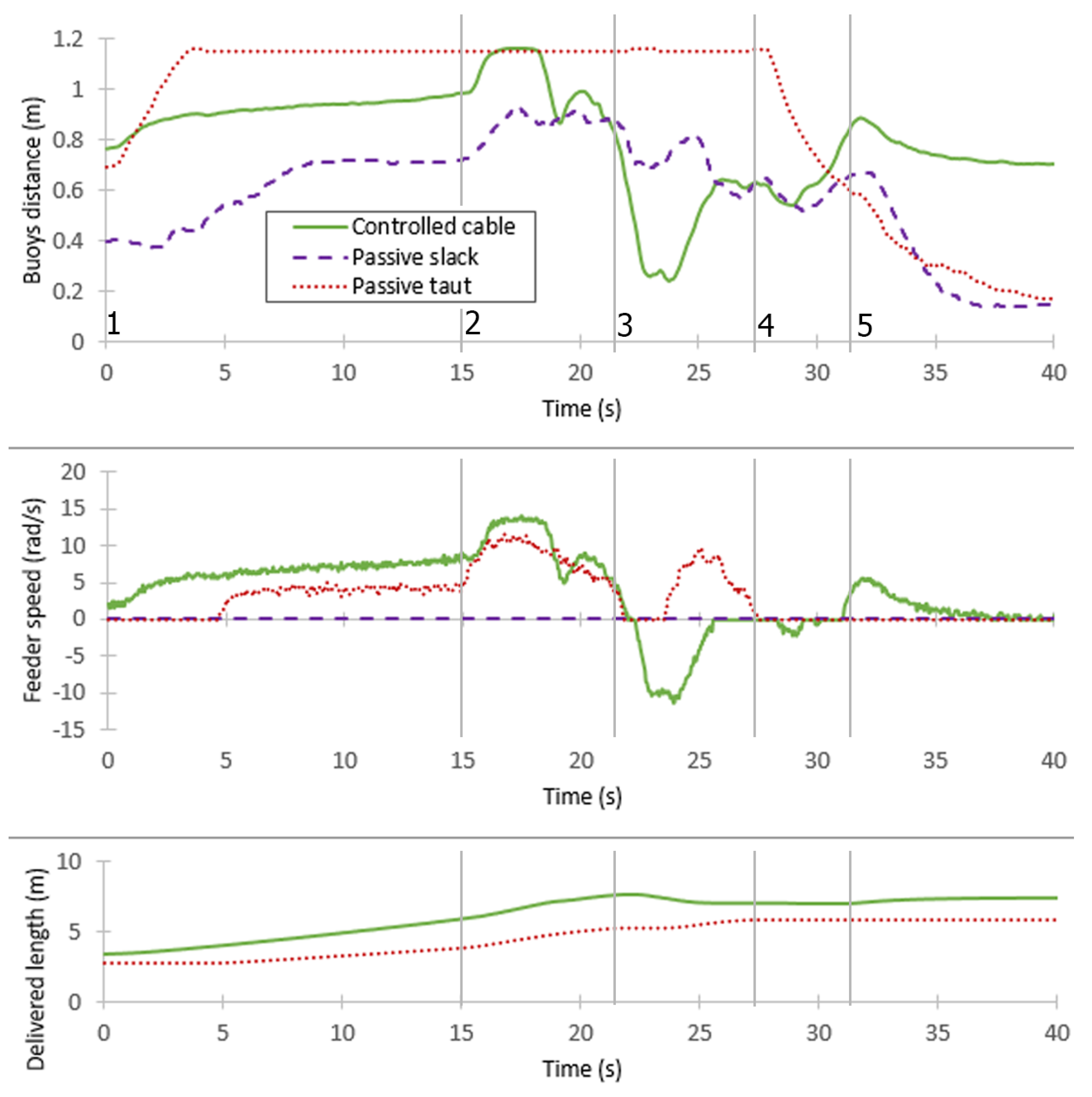
4.3. Trajectories
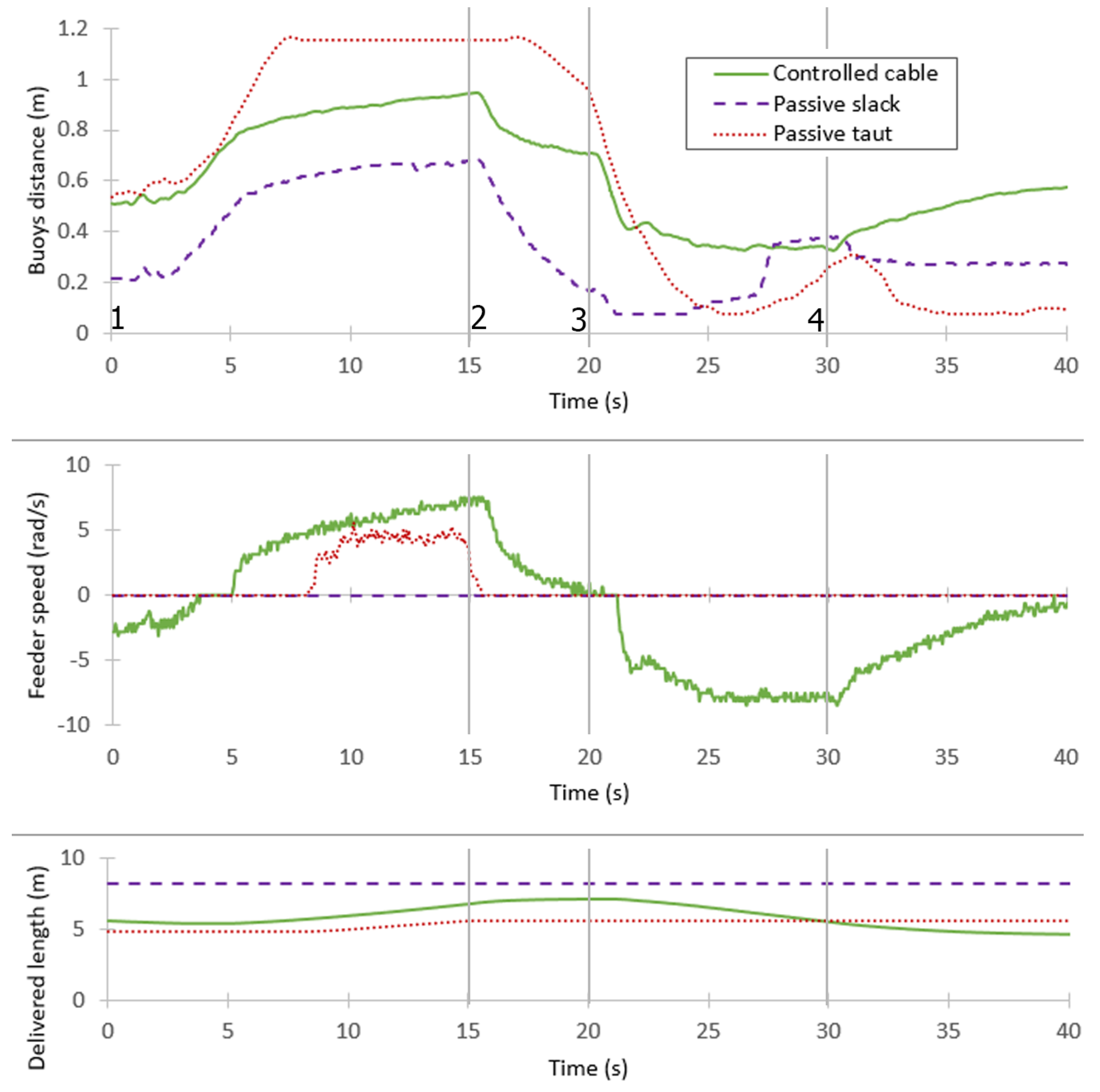
- A linear trajectory where the ROV goes forwards and then backwards First, a forward thrust command of is sent for 15 s (between keyframes 1 and 2). Then, a zero command is sent for 5 s (between points 2 and 3). Finally, a backward thrust command of is sent for 10 s (between points 3 and 4).
- A curvilinear S-shape trajectory comprising the following steps:
- -
- a forward thrust of 40% for 15 s (between points 1 and 2);
- -
- a right turn composed of a yaw thrust of combined with a forward thrust of for 6.5 s to turn right (between points 2 and 3);
- -
- a left turn with the same thrust command values as the left turn, for 6 s (between points 3 and 4);
- -
- a forward thrust of for 4 s (between points 4 and 5).
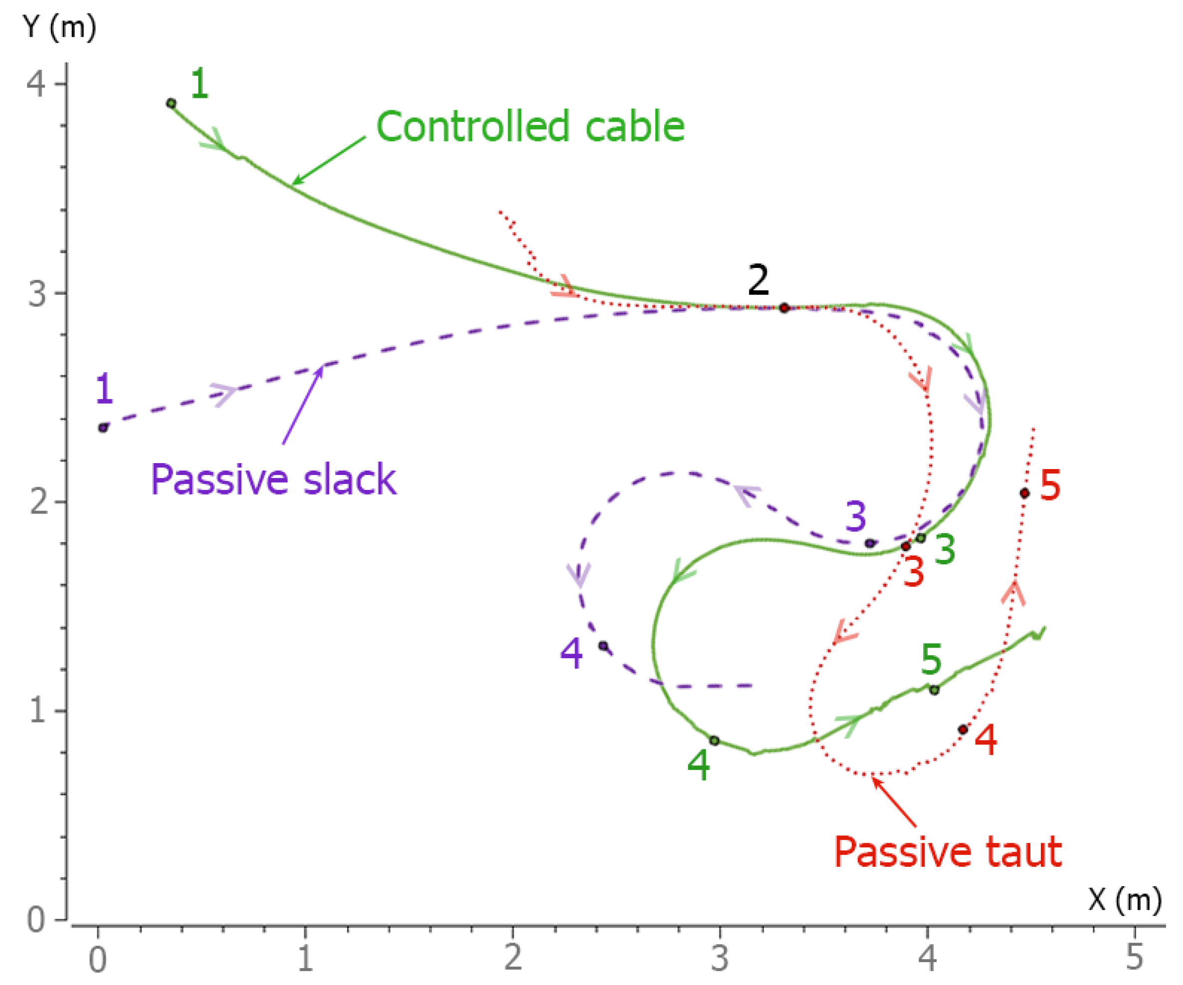
- Passive slack cable, where cable of sufficient length was deployed in the water from the beginning.
- Passive taut cable, where the cable is stretched between the feeder and the ROV when the ROV moves away from the feeder, which means that the buoy–ballast system is also completely stretched and has no real influence on the ROV. The feeder is not powered. When the ROV comes closer to the feeder, the cable is no longer taut, and the buoy gap tends to be reduced to a minimum.
- Cable control, using buoy gap control mode. A and forward thrust is associated with a buoy gap of about 0.7 mn and 0.8 m, respectively, according to the steady-state model.
5. Results And Discussion
5.1. Linear Trajectory
5.2. Curvilinear Trajectory
6. Conclusions
- The simulations and the experiments conducted with a BlueROV and a neutral cable demonstrated the validity of the concept. The steady-state model was used in the control loop to obtain a target distance between the buoys from the ROV speed command. The feeder appeared to react as expected with respect to the command speeds of the ROV.
- The shape of the cable was kept in a semi-stretched configuration during the experiments of linear and curved trajectories.
- This solution is easy to set up and can be useful in preventing the cable from pulling on the ROV, thus avoiding entanglement of the cable with its surroundings.
Author Contributions
Funding
Informed Consent Statement
Data Availability Statement
Acknowledgments
Conflicts of Interest
Appendix A. Statics Analysis of the Buoy–Ballast System
- is the cable bending torque exerted onto the branch at , and is the cable bending torque exerted onto the branch at .
- and are the cable bending torques exerted by the right and left parts, resp., at C.
References
- Christ, R.; Wernli, R. The ROV Manual a User Guide for Remotely Operated Vehicles, 2nd ed.; Elsevier: Amsterdam, The Netherlands, 2014. [Google Scholar]
- Khatib, O.; Yeh, X.; Brantner, G.; Soe, B.; Kim, B.; Ganguly, S.; Stuart, H.; Wang, S.; Cutkosky, M.; Edsinger, A.; et al. Ocean one: A robotic avatar for oceanic discovery. IEEE Robot. Autom. Mag. 2016, 23, 20–29. [Google Scholar] [CrossRef]
- Destelle, J.J.; Vallée, C. The MEUST infrastructure for neutrino astronomy. Nucl. Instrum. Methods Phys. Res. Sect. A Accel. Spectrometers Detect. Assoc. Equip. 2013, 725, 227–229. [Google Scholar] [CrossRef]
- Capocci, R.; Dooly, G.; Omerdić, E.; Coleman, J.; Newe, T.; Toal, D. Inspection-Class Remotely Operated Vehicles—A Review. J. Mar. Sci. Eng. 2017, 5, 13. [Google Scholar] [CrossRef]
- Ajwad, S.A.; Iqbal, J. Recent Advances and applications of tethered robotic systems. Sci. Int. 2014, 26, 2045–2051. [Google Scholar]
- Tortorici, O.; Anthierens, C.; Hugel, V.; Barthelemy, H. Towards active self-management of umbilical linking ROV and USV for safer submarine missions. IFAC-PapersOnLine 2019, 52, 265–270. [Google Scholar] [CrossRef]
- McLain, T.W.; Rock, S.M. Experimental Measurement of ROV Tether Tension. In Proceedings of the ROV’92, San Diego, CA, USA, 10–12 June 1992; p. 6. [Google Scholar]
- Bevilacqua, L.; Kleczka, W.; Kreuzer, E. On the Mathematical Modeling of ROV’S. IFAC Proc. Vol. 1991, 24, 51–54. [Google Scholar] [CrossRef]
- Soylu, S.; Buckham, B.J.; Podhorodeski, R.P. Dynamics and control of tethered underwater-manipulator systems. In Proceedings of the OCEANS 2010 MTS/IEEE SEATTLE, Seattle, WA, USA, 20–23 September 2010; pp. 1–8. [Google Scholar]
- Fang, M.C.; Hou, C.S.; Luo, J.H. On the motions of the underwater remotely operated vehicle with the umbilical cable effect. Ocean Eng. 2007, 34, 1275–1289. [Google Scholar] [CrossRef]
- Feng, Z.; Allen, R. Evaluation of the effects of the communication cable on the dynamics of an underwater flight vehicle. Ocean Eng. 2004, 31, 1019–1035. [Google Scholar] [CrossRef]
- Gay Neto, A.; de Arruda Martins, C. Structural stability of flexible lines in catenary configuration under torsion. Mar. Struct. 2013, 34, 16–40. [Google Scholar] [CrossRef]
- Coyne, J. Analysis of the formation and elimination of loops in twisted cable. IEEE J. Ocean. Eng. 1990, 15, 72–83. [Google Scholar] [CrossRef]
- Drumond, G.; Pasqualino, I.; Pinheiro, B.; Estefen, S. Pipelines, risers and umbilicals failures: A literature review. Ocean Eng. 2018, 148, 412–425. [Google Scholar] [CrossRef]
- Brignone, L.; Raugel, E.; Opderbecke, J.; Rigaud, V.; Piasco, R.; Ragot, S. First sea trials of HROV the new hybrid vehicle developed by IFREMER. In Proceedings of the OCEANS 2015—Genova, Genova, Italy, 18–21 May 2015; pp. 1–7. [Google Scholar]
- Viel, C. Self-management of the umbilical of a ROV for underwater exploration. Ocean Eng. 2022, 248, 110695. [Google Scholar] [CrossRef]
- Frank, J.E.; Geiger, R.; Kraige, D.R.; Murali, A. Smart Tether System for Underwater Navigation and Cable Shape Measurement. U.S. Patent US8437979B2, 7 May 2013. [Google Scholar]
- Duncan, R.G.; Froggatt, M.E.; Kreger, S.T.; Seeley, R.J.; Gifford, D.K.; Sang, A.K.; Wolfe, M.S. High-accuracy fiber-optic shape sensing. In Proceedings of the SPIE Smart Structures and Materials + Nondestructive Evaluation and Health Monitoring, San Diego, CA, USA, 18–22 March; p. 65301S.
- Xu, C.; Chen, J.; Yan, D.; Ji, J. Review of Underwater Cable Shape Detection. J. Atmos. Ocean. Technol. 2016, 33, 597–606. [Google Scholar] [CrossRef]
- Xu, C.; Wan, K.; Chen, J.; Yao, C.; Yan, D.; Ji, J.; Wang, C. Underwater cable shape detection using ShapeTape. In Proceedings of the OCEANS 2016 MTS/IEEE Monterey, Monterey, CA, USA, 19–23 September 2016; pp. 1–4. [Google Scholar]
- Banerjee, A.K.; Do, V.N. Deployment control of a cable connecting a ship to an underwater vehicle. J. Guid. Control. Dyn. 1994, 17, 1327–1332. [Google Scholar] [CrossRef]
- Zhao, C.; Thies, P.R.; Johanning, L. Investigating the winch performance in an ASV/ROV autonomous inspection system. Appl. Ocean Res. 2021, 115, 102827. [Google Scholar] [CrossRef]
- Raugel, E.; Opderbecke, J.; Fabri, M.; Brignone, L.; Rigaud, V. Operational and scientific capabilities of Ariane, Ifremer’s hybrid ROV. In Proceedings of the OCEANS 2019—Marseille, Marseille, France, 17–20 June 2019. [Google Scholar]
- Zhou, H.; Cao, J.; Yao, B.; Lian, L. Hierarchical NMPC–ISMC of active heave motion compensation system for TMS–ROV recovery. Ocean Eng. 2021, 239, 109834. [Google Scholar] [CrossRef]
- Lubis, M.B.; Kimiaei, M.; Efthymiou, M. Alternative configurations to optimize tension in the umbilical of a work class ROV performing ultra-deep-water operation. Ocean Eng. 2021, 225, 108786. [Google Scholar] [CrossRef]
- Laranjeira, M.; Dune, C.; Hugel, V. Catenary-based visual servoing for tether shape control between underwater vehicles. Ocean Eng. 2020, 200, 107018. [Google Scholar] [CrossRef]
- Tortorici, O.; Anthierens, C.; Hugel, V. A new flex-sensor-based umbilical-length management system for underwater robots. In Proceedings of the European Conference on Mobile Robotics, Coimbra, Portugal, 4–7 September 2023. [Google Scholar]


| Physical Parameters | Fathom Slim Tether | Unit |
|---|---|---|
| Axial stiffness | * | N |
| Axial damping | * | kg.m/s |
| Bending stiffness | /rad | |
| Bending damping | * | /rad |
| Torsion stiffness | /rad | |
| Torsion damping | * | /rad |
| Linear density | kg/m | |
| Drag coefficient | * | - |
| Radius | m | |
| Breaking strength | 1520 | N |
| Overall buoyancy | Neutral |
| Distance between ballast and buoy | 0.6 m |
| Buoy size | 29 × 29 × 47 |
| Buoy foam density | 288 |
| Ballast mass | 76 g |
| Ballast diameter | 25 mm |
| Flex sensor model | FS-L-0095-103-ST (Spectra Symbol) |
| Flex sensor size | 110 mm long, 0.5 mm thick |
Disclaimer/Publisher’s Note: The statements, opinions and data contained in all publications are solely those of the individual author(s) and contributor(s) and not of MDPI and/or the editor(s). MDPI and/or the editor(s) disclaim responsibility for any injury to people or property resulting from any ideas, methods, instructions or products referred to in the content. |
© 2024 by the authors. Licensee MDPI, Basel, Switzerland. This article is an open access article distributed under the terms and conditions of the Creative Commons Attribution (CC BY) license (https://creativecommons.org/licenses/by/4.0/).
Share and Cite
Tortorici, O.; Péraud, C.; Anthierens, C.; Hugel, V. Automated Deployment of an Underwater Tether Equipped with a Compliant Buoy–Ballast System for Remotely Operated Vehicle Intervention. J. Mar. Sci. Eng. 2024, 12, 279. https://doi.org/10.3390/jmse12020279
Tortorici O, Péraud C, Anthierens C, Hugel V. Automated Deployment of an Underwater Tether Equipped with a Compliant Buoy–Ballast System for Remotely Operated Vehicle Intervention. Journal of Marine Science and Engineering. 2024; 12(2):279. https://doi.org/10.3390/jmse12020279
Chicago/Turabian StyleTortorici, Ornella, Charly Péraud, Cédric Anthierens, and Vincent Hugel. 2024. "Automated Deployment of an Underwater Tether Equipped with a Compliant Buoy–Ballast System for Remotely Operated Vehicle Intervention" Journal of Marine Science and Engineering 12, no. 2: 279. https://doi.org/10.3390/jmse12020279
APA StyleTortorici, O., Péraud, C., Anthierens, C., & Hugel, V. (2024). Automated Deployment of an Underwater Tether Equipped with a Compliant Buoy–Ballast System for Remotely Operated Vehicle Intervention. Journal of Marine Science and Engineering, 12(2), 279. https://doi.org/10.3390/jmse12020279