Recording the SS Thistlegorm: Rapid Multi-Image Underwater Photogrammetric Survey of a Large Second World War Wreck

Abstract

This paper describes the workflow followed to survey and monitor the interior and exterior of a large and complex metal wreck, the SS Thistlegorm in the Red Sea, using digital photogrammetry. Utilizing a simple single-camera rig and off-the-shelf software, this study presents a cost-effective and easily replicable method for monitoring change in metal wrecks that meets professional standards and can involve non-specialists in data collection. This paper details the background of the SS Thistlegorm, the equipment used, and the photogrammetric surveys conducted in 2017 and 2022. It outlines the importance of having a clearly thought-out data-management system when working on a large target recorded over a limited series of dives. In particular, this paper considers testing the accuracy of the data obtained and describes the post-processing workflow in detail. The conclusion underscores the feasibility of achieving an accurate geo-referenced baseline 3D survey with readily available equipment and how these data can contribute to historical research and ongoing monitoring efforts.

1. Introduction

Using the SS Thistlegorm as a case study, this paper outlines the simple, low-cost, single-camera photogrammetry approach taken to survey wrecks in the Red Sea as part of the monitoring work of the Wreck at Risk project. Wrecks at Risk is a collaboration between the University of Edinburgh and the Centre of Maritime Archaeology at the University of Alexandria. It set out to survey a range of popular tourist wrecks in the Egyptian Red Sea to illustrate their importance as underwater cultural heritage and to encourage good diving practices to prolong their preservation as historic assets of value to the local Egyptian economy.

There have been studies of specialized approaches to photogrammetric surveys involving multi-camera rigs and arrays [1,2,3,4], but the approach discussed here is focused on a simple single-camera rig using standard off-the-shelf equipment and software. Given the often limited resources of archaeological projects, this is not only the most common way work is carried out in the field but also more readily allows the involvement of non-specialists in collecting data suitable for photogrammetric processing. A key aim of the Wrecks at Risk project is to develop a rapid, easily repeatable, and cost-effective method that can incorporate data collected by recreational divers to help monitor sites over time.

Approaches for carrying out low-cost single-camera photogrammetry on shipwreck sites have been presented before [5,6,7], but this paper differs in that it describes the recording of an extensive and complex 3D structure, covering the internal decks and external areas of a very large, upstanding metal wreck, within a limited timeframe. Since completing the baseline survey of the Thistlegorm in 2017, we have often been asked how we managed to survey such a large wreck in such a short space of time and what steps we took to ensure the accuracy of our work. In contrast to previous works, which have tended to focus on relatively small wrecks with flat relief [1,8,9,10,11,12,13,14], the SS Thistlegorm survey covered a significantly larger subject—the wreck of a ship originally measuring 4900 grt, 131.6 m × 17.7 m × 7.6 m, resting in depths ranging from 12 msw (meters of sea water) to 32 msw. The main survey was conducted using a single camera across 12 dives, with a total diver time of 13 h and 45 min. The majority of the areas were surveyed in 2017, with the Captain’s House covered on a single dive in June 2018 (see

Table 1. Total area surveyed over 12 dives.

Location	Area	Number of Images
Outer surfaces—ship and seabed	21,600 m2	14,183
Forecastle room	469 m2	986
Deck 1—Holds 1 and 2	1870 m2	5554
Deck 2—Holds 1 and 2	2810 m2	4218
Deck 1—Hold 3	919 m2	1460
Saloon House	313 m2	925
Engine Room—partial	708 m2	462
Captain’s House	138 m2	302
Total Survey Area	28,827 m2	28,053

). A second survey season in 2022 allowed us to further test the accuracy of the model as well as identify any changes to the structural integrity of the wreck and its cargo over the intervening five years.

The method of gathering data in the field is outlined, with emphasis on the importance of camera calibration, proper lighting of underwater subjects using strobes to obtain true-color images, and the significance of in-water measurements to ensure accurate scaling of the survey. Following the acquisition of high-quality images in the water, the most important aspect in the creation of large photogrammetric surveys is the organization and management of the data during post-processing. We outline a post-processing workflow using cloud capacity and flexibility. The main considerations for achieving accurate results are discussed, acknowledging that any survey involves a trade-off between accuracy and the time and effort required to collect data. Our objective is to present a cost-effective, time-efficient method for recording the exterior and interiors of a large and complex wreck that yields an acceptable level of measurable accuracy to be considered an effective archaeological survey to serve as a baseline for future monitoring of a site [15].

2. SS Thistlegorm: Background

Of all-steel construction, the five-hold cargo steamship SS Thistlegorm was launched into the River Wear at Sunderland on 9 April 1940. Almost immediately contracted for the war effort, she was fitted with a 4-inch (101.6 mm) anti-aircraft gun and a heavy-caliber, low-angle gun to the stern and classified as a Defensively Equipped Merchant Ship (DEMS). For her fourth and final voyage in May 1941, the Thistlegorm was loaded with a mixed cargo of lorries, motorbikes, aircraft spares and airfield equipment, universal carriers, and ammunition in Glasgow, with a final destination of Alexandria, Egypt. On the night of the 6 October 1941, whilst at anchor at the Straits of Gubal in the Red Sea (Figure 1), the ship was attacked by a pair of German Heinkel He 111 bombers with at least one bomb hitting Hold No. 4 [16]. The resulting fire triggered a secondary explosion in the cargo of ammunition, destroying the hold and sinking the ship. From a crew of 41, 5 gunners and 4 sailors lost their lives during either the initial attack, fire, secondary explosion, or subsequent sinking.

At the time of construction, the Thistlegorm was recorded as being 131 m long with a gross tonnage of 4898.13 grt and a total cargo space of 7782 cubic meters. The wreck now rests on a seabed featuring low-lying rocky outcrops interspersed with patches of fine sand at a depth of 32 msw. Physically large, the wreck of the SS Thistlegorm is subject to strong currents and variable underwater visibility ranging from 10–15 m to 25–30 m. The bow and midship sections of the wreck remain upright and largely intact, while the stern section has collapsed to the port side. Between both sections lie the shattered remains of Holds No. 4 and 5, where a spread-out and structurally complex debris field testifies to the massive explosion that took the vessel to the bottom (Figure 2 and Figure 3).

As part of the broader Wrecks at Risk project, the SS Thistlegorm survey had three main objectives: (1) to create an accurate 3D model of the site, raising awareness of the historical importance of the wreck; (2) to record and identify the cargo of the vessel [16]; and (3) to document the current state of preservation and establish a baseline survey of the site for monitoring changes over time. Due to the sheer size and detail of the wreck and the complexity of the interior spaces, the survey of the SS Thistlegorm was a massive undertaking that pushed current underwater photogrammetry capabilities to their limits.

3. Equipment and Methodology

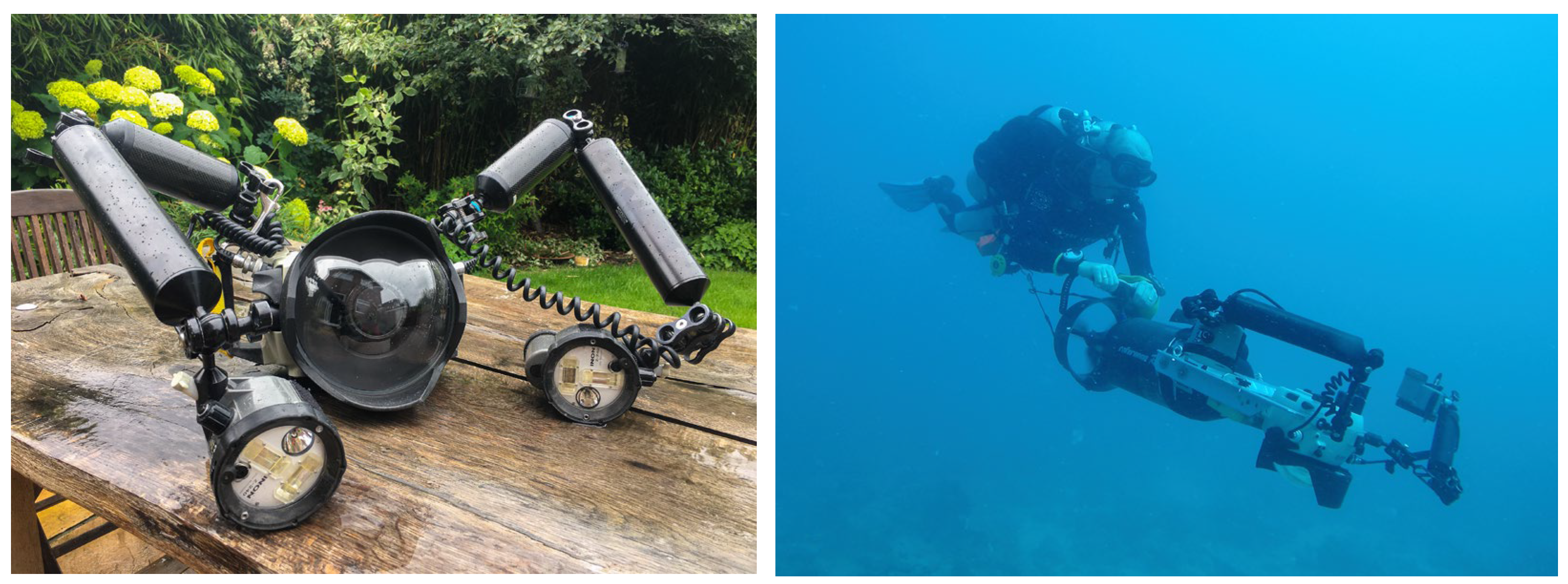
All of the images in 2017 and the majority in 2022 were captured using a Nikon D700 SLR body (Nikon Corp., Tokyo, Japan) with a Nikon 16 mm fisheye lens encased in a Subal underwater camera housing (Subal GmBH, Vienna, Austria). All shots were illuminated with artificial light using—in this case, two Inon z240 strobes (Inon Inc. Tokyo, Japan) (Figure 4).

Additional still image datasets were captured during the 2022 fieldwork using a Sony A7Siii with a 16~35 mm zoom lens (Sony Group, Tokyo, Japan) in an Isotta housing (Isotecnic srl, Milano, Italy) using Hydra 8000 Kraken strobes (Kraken Sports, London, ON, Canada) and an Olympus TG20 (Olympus Corp., Shinjuku-Ku, Japan). For some comparative work, stills extracted from GoPro 7 (GoPro Inc., San Mateo, CA, USA) action camera video using default settings were used to create a basic mesh and orthomosaic recording of the “as-is” condition for comparison to the 2017 baseline survey.

In these instances, the equipment used, such as the use of a zoom lens (not recommended for photogrammetry) and the technique of frame extraction from video, should only be used with caution and/or when no other alternative is available. Nevertheless, the value for comparative work in reviewing changes between the high-definition robust 2017 survey with lesser-quality datasets is sufficient to track differences and changes over time.

Any survey or model is only as good as the data collected, and in photogrammetry, this means choosing the right camera set-up to capture good, clear, and well-lit photos [7]. Although there is a range of acceptable solutions from which archaeologists can choose, the best results depend heavily on the equipment used. Zhukovsky et al. (2013) discuss constraints in underwater photography, which include optical distortions caused by water and camera interface, optical noise caused by moving interfering objects; such as swimming fishes or suspension in the water (backscatter); low visibility; and lack of light; which changes the colors [17].

A rule of thumb in underwater photography is to get as close as possible to the subject, and for multi-image photogrammetry, this remains true with the caveat you also need to achieve sufficient overlap of the subject between photos and still cover enough ground. Overlap between adjacent images should ideally be 70~80%, thus enabling photogrammetry software to identify evenly distributed tie points. There is no upper amount of tie points (Metashape has a user setting defaulted to 4000), but a lower limit of >100 tie points with even distribution is considered a lower limit for robust reconstruction. Higher overlap between adjacent frames may result in extended processing duration for no extra benefit. Less overlap can induce curvature over greater distances, and higher overlap increases processing time with little or no benefit to the outputs.

The accuracy and quality of reconstruction are further influenced by the image quality. Source images must be free of noise, free of motion blur, and in focus to enable accurate matching of key points between overlapping frames.

For underwater photogrammetry, the best possible compromise involves the use of wide-angle lenses together with a hemispheric dome. Cameras with close-focus, wide-angle lenses eliminate as much water as possible between sensor and target, ensuring wide coverage of the area being recorded, while the hemispheric dome provides sharper image corners when using such wide-angle optics. Close-focus wide-angle lenses, typically with a focal length <28 mm (full-frame sensor) or fisheye lenses, are used for underwater photography. Focus distances of 20 cm or less reduce the amount of water between the camera sensor and the subject, reducing the quantity of artificial light required to illuminate the subject. Once the light enters the lens, the path taken to the sensor should remain stable and consistent between frames, and reducing variability is highly desirable. Photogrammetric software such as Metashape and 3DF Zephyr carry basic calibration parameters for a wide range of frame and fisheye lenses and will calculate individual calibration for a given camera group during the alignment stage. For this reason, a lens with stable, unchanging, and fixed characteristics is preferred.

Digital cameras are equipped with one of two types of sensors: either a Charged Coupled Device (CCD) or a Complementary Metal Oxide Semiconductor (CMOS). Both devices convert visible light into an electrical signal. The physical differences are beyond the scope of this paper, with the exception of one characteristic that may impact photogrammetry: the shutter type. CMOS sensors are a “rolling shutter” where each row of photo sensors is exposed in turn, typically starting at the top of the sensor and ceasing at the bottom. Thus, the read of light value “rolls” incrementally across the sensor. As a result, any movement in the camera during the rolling read can translate into model distortion. Instead, CCD sensors read the array of photosensors in a single event that starts and stops simultaneously. Exposure control is managed by a mechanical shutter, and with a single event reading the light values, the risk of motion-induced blur is reduced. For this reason, a CCD sensor and mechanical shutter are preferred when gathering source images for photogrammetry.

The selective loss of colors with depth and the low light levels frequently verified underwater call for the use of strobe lights. Ideally, two strobe lights spread out with long articulated arms create the best and most flexible equipment arrangement for multi-image photogrammetry. The hard shadows cast by strobe lights must be controlled, however, because they change position from image to image and affect the stability of colors in the subject materials during model reconstruction. The position of any artificial lighting is critical to produce an even and consistent light and to reduce the presence of backscatter in the captured image. Backscatter is caused by suspended particles in the water column being illuminated by the strobe light. Each strobe should be placed behind the dome port shade and aligned with the rear of the camera housing along the X axis of the camera sensor. This position reduces the presence of the intense cone of light that is created immediately in front of the strobe.

Although, as McCarthy and Benjamin (2014) rightly point out, consumer-grade compact cameras produce images from natural light underwater, even in dark environments [5], we would argue the results are far from optimal and can significantly undermine the quality and accuracy of the models produced. Effective lighting of scenes provides true color recording and avoids the creation of blue/green images that later need to be artificially adjusted. Not only that, well-lit scenes produce more accurate results as more detail is visible from photo to photo and avoid the creation of blue/green models that, due to decreased accuracy induced by a low number of overlapping key points, can suffer from bowling effects resulting in “banana-shaped” ship models. Artificial illumination has yet a further benefit; when working in very low light, the intense burst of light emitted by the strobes can help “freeze” the image detail and reduce camera shake-induced motion blur. The inherent motion-damping properties of water can mitigate the impact, with handheld shutter speeds as low as 1/10th possible, but for most handheld work, a minimum shutter speed of 1/60th was set. With the primary source of lighting intended to be artificial, the camera white balance can be set and controlled manually. Thistlegorm images were shot with the camera using a fixed white balance value of 5560 K, matching the color temperature of the strobes. Matching white balance of the lighting source can assist during post-processing and remove the requirement to manually correct or adjust the source image color settings. For stability and predictability of image results, manual camera settings (ISO, aperture, shutter speed, all chosen to suit underwater conditions) were set and checked at regular intervals during the dive.

Curvature in models, described as bowl or banana-shaped, is a highly undesirable feature of both terrestrial and underwater photogrammetry. The causes are typically:

• Missing or highly inaccurate ground control point constraints;
• Overlap of the source images does not provide sufficient information for robust lens calibration;
• Overlap of the source images does not provide sufficient opportunity to detect and robustly align tie points;
• Source images contain extensive areas of textureless subject material where potential tie points cannot be detected;
• The lens is working with autofocus and/or image stabilization enabled.

Linear mapping missions with three or fewer passes may induce issues described in 2. With autofocus disabled, fixing the internal lens parameters mitigates induced errors by 3. Finally, ground control points add stability and, in the case of the reconstruction of the Thistlegorm, have been appropriately weighted to reflect the accuracy of the hardware available.

Autofocus was used at the beginning of the survey to set the initial focus and then turned off, with the camera-to-subject distance, typically between 1 m or 2 m, held constant throughout survey dives (only dropping below the 1 m threshold when physical space, such as when working in the cargo holds, dictated). High levels of ambient light permitted the use of lens autofocus, but this feature was not used to avoid issues with missed or delayed focus lock, which can affect the timing of images, sometimes creating excessive gaps between images, resulting in alignment failures in photogrammetry processing.

With a Nikon D700 (sensor 36 mm wide with 4256 pixels) and 16 mm (focal length) lens, the Ground Sampling Distance (the amount of seabed covered by a single image and expressed as a linear measurement or distance between two adjacent pixels) is:

1 m distance:

1 × 36 = 0.53 mm per pixel

16 × 4256

2 m distance:

2 × 36 = 1.06 mm per pixel

16 × 4256

The digital equivalent of film ISO settings—the measure of sensitivity—permits the adjustment and balancing of available and artificial light to produce an image suitable for photogrammetry. However, higher ISO settings can introduce an effect known as noise into the individual images. Noise introduces elements into the recorded image that photogrammetric software can record and recognize as common features and be used to (mis)align images.

Therefore, to avoid noise, the ISO setting applied is as low as practically possible. The level at which noise starts to manifest will depend on the camera design, sensor type, and size of the sensor itself. Typically, larger sensors, such as those replicating the format of 35 mm film cameras, permit higher ISO values to be used than their cropped (DX) sensor equivalent.

Camera motion, though restricted by virtue of being surrounded by water, can affect the sharpness of images—in an environment subject to high levels of ambient light, combined with a slow shutter speed (approx. < 1/60th), motion blur may occur. As mentioned above, the use of strobes for artificial illumination can mitigate the risk of motion blur, but the primary and main method is to use a minimum shutter speed of 1/60th and preferably higher.

4. Photogrammetric Survey 2017

The first season was carried out in 12 dives over 5 days between 30 June and 4 July 2017 and set out to establish a baseline survey of the exterior of the wreck, main interior spaces (upper and lower decks of Holds No. 1 and 2, Saloon House, Wheelhouse, and Forecastle Room) and the cargo. A total of 24,307 wide-angle images, representing 637 Gb of data, were captured during this season from a total of 806 min or 13 h and 43 min in-water time. Subsequently, the source images for the Captain’s Room survey were collected during one dive on 1 July 2018.

All dives were conducted on Enriched Air Nitrox 32 (32% oxygen and 68% nitrogen mix) to maximize bottom time and minimize diver fatigue over repeated dives. As the remains to be surveyed ranged from 12 msw to 32 msw deep, the Thistlegorm was ideally suited to the use of nitrox and twin tanks. Given the use of nitrox, the main limiting factor in gathering data on single dives proved to be the battery life of both the camera and the strobes rather than gas consumption or decompression obligations.

On-site data processing to validate captured data was carried out using Agisoft Photoscan Professional running on a MacBook Pro laptop. Scaling and validation of the 3D model as it was constructed were applied using direct measurements taken from the wreck, with additional checking and validation confirmed post-fieldwork by comparison of components and features to those in the original builder’s plans. Latitude, longitude, and depth values of key points on the wreck were recorded and applied to the 3D model, applying additional constraints and geo-location.

The physical effort of scanning the exterior of the wreck was eased by mounting the camera on an underwater scooter or diver propulsion vehicle (DPV). The mount comprised an aluminum frame secured with stainless steel fastenings, designed to slide over the DPV battery compartment and secured by two webbing straps (Figure 4). Additional foam was added to compensate for the negative buoyancy of both aluminum sections, housed DSLR camera, and strobes, with the result that in the water, the DPV and camera combination was as close to neutrally buoyant as possible. Setting the camera interval timer to 1 Hz, on a single dive, 2500~4000 images could be shot in sequence with the pace of the DPV adjusted to ensure optimum image overlap was obtained. DPV velocity over ground required constant monitoring as diurnal tidal cycles at the Thistlegorm created currents strong enough to affect the overlap.

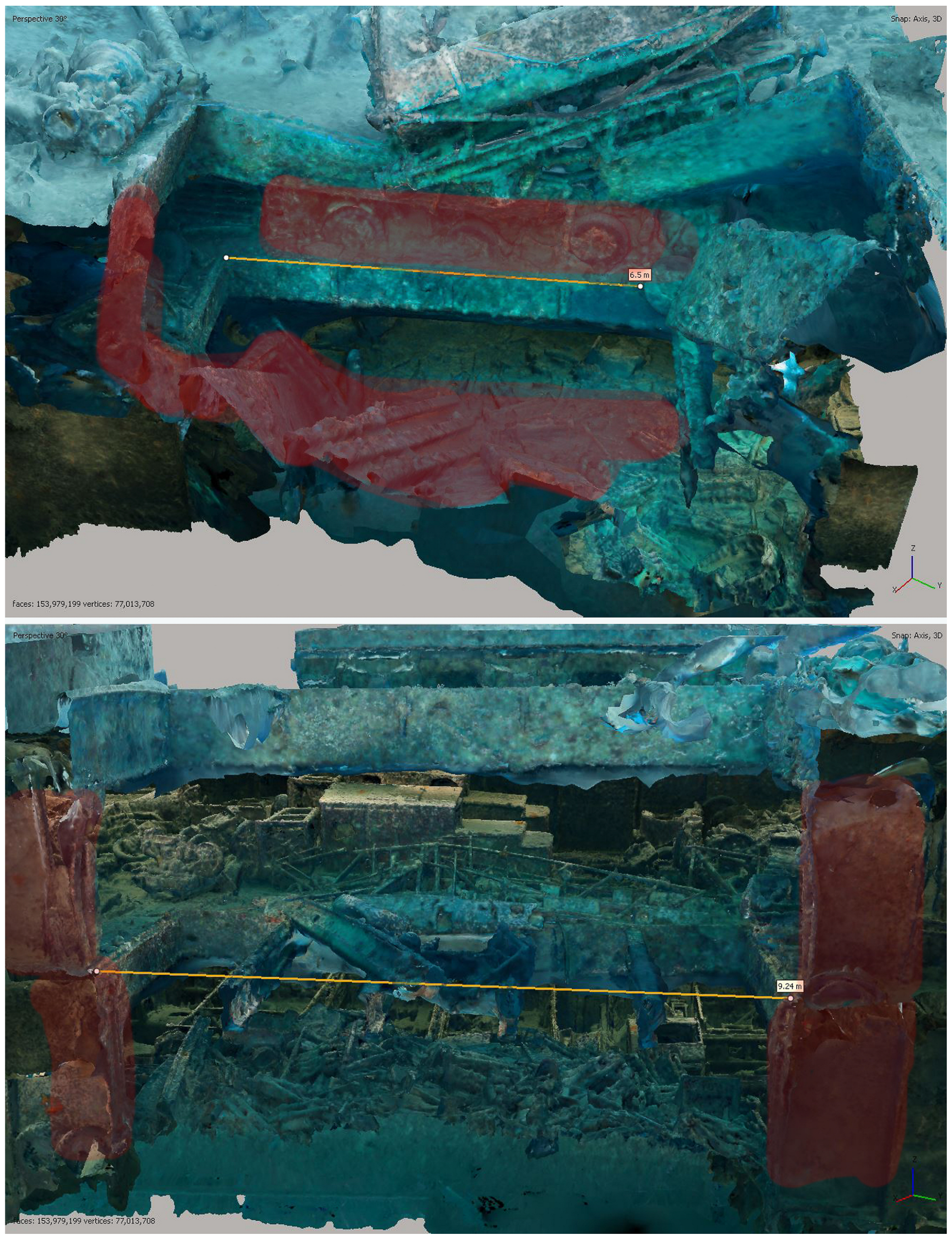
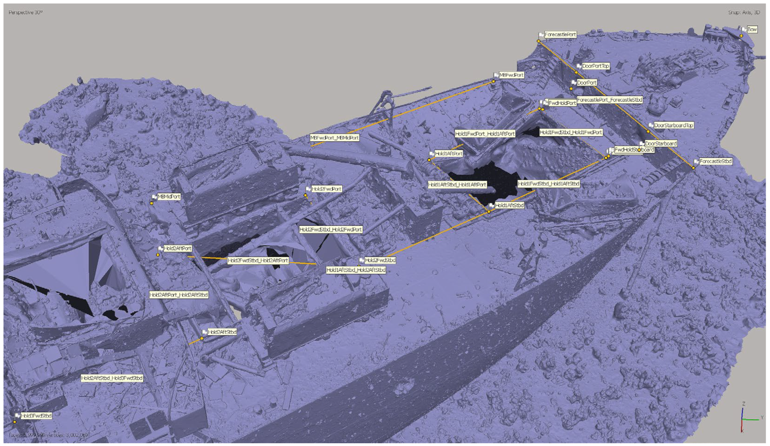
With the outside covered and a draft model built, surveying the holds and their cargo commenced. Particular attention was paid to the joining points between the decks to ensure the separate scans would align later. As a complex 3D structure, the original ship’s structure of vertical supports between decks and the now-collapsed hold covers of Hold No. 1 were used to tie the main, upper, and lower decks into a single set of aligning images (Figure 5).

The remains of the lorries, motorbikes, and aircraft parts, all packed into the cramped space of the holds, presented their own unique set of issues, especially in keeping the camera aligned parallel with the surface being captured in tight spaces. A frequent problem was other divers and their bubbles appearing in the images—the wreck is very popular—and having moving objects in the images can cause alignment issues. Scanning the cargo hold decks took a total of 5 dives to complete (Figure 6 and Figure 7).

The external surfaces of the wreck and each section listed in Table 1 were processed as separate model chunks. Internal areas, such as the cargo holds, were processed and included approximately 200 images that were used to reconstruct the main deck areas around the hold entrances. The main wreck model was aligned, optimized, scaled, and geo-referenced first, and each interior space was processed separately. Each of the separate chunks contained a common set of cameras shared with the main wreck, permitting the use of the Cameras method to Align Chunks. Shared cameras in separate chunks were aligned, positioned, and scaled relative to the main wreck model.

For increased accuracy and for geolocation, features and points were physically measured underwater using tapes, and these measurements were then added to the model. GPS data gathered on the site enabled global geolocation with positions of key features of the wreck recorded and applied to the final model. The availability and use of GPS equipment in the South Sinai Governorate of Egypt can be subject to severe restrictions. Thus, due to the equipment available, the tolerance of recorded latitude and longitude measurements was factored to ±5 m.

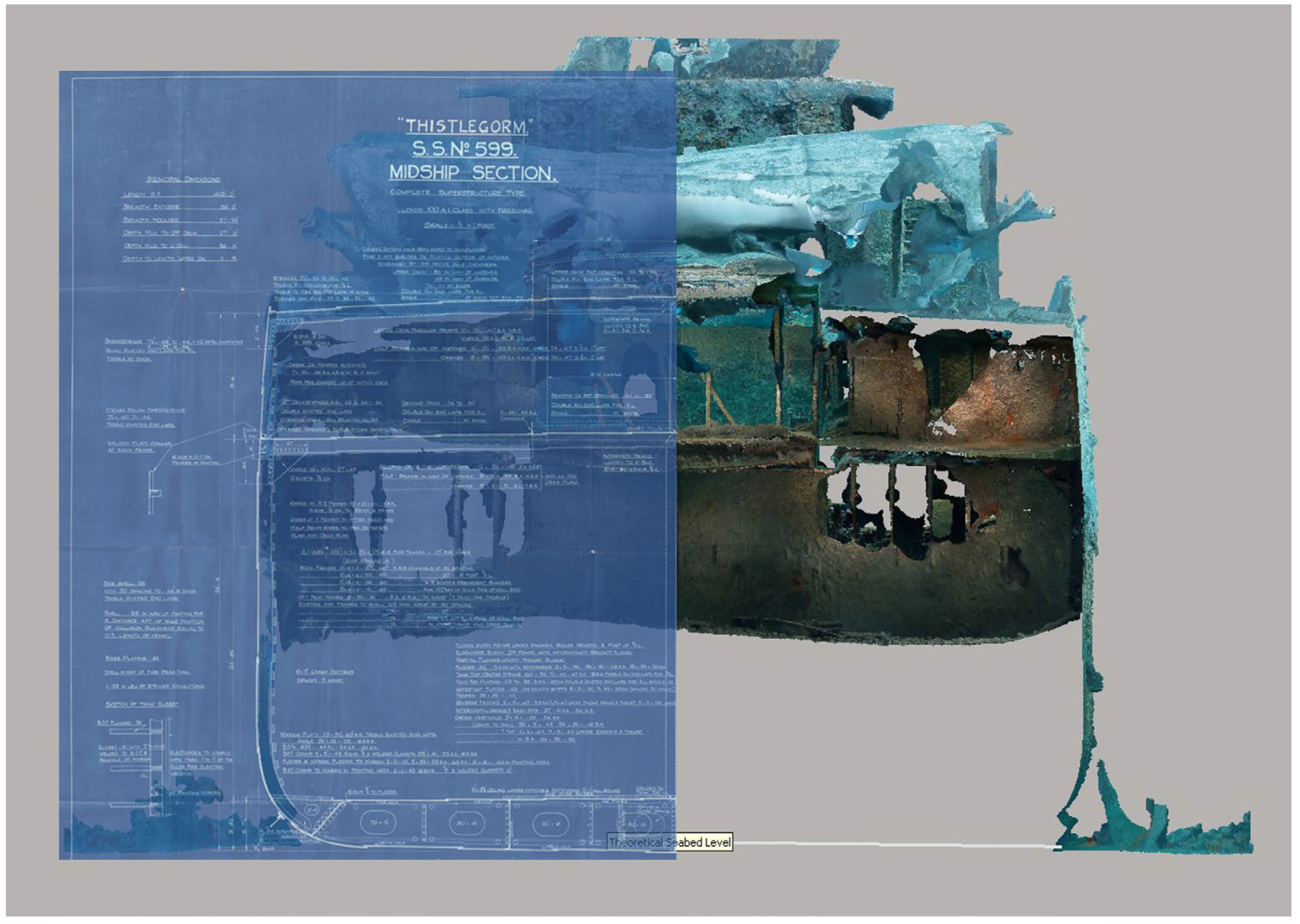
Subsequent to the 2017 fieldwork, the Thistlegorm builder’s plans were located in the Tyne and Wear Archives. Physical measurements taken from the as-constructed plans were used to validate field measurements and were later used to add additional constraints to the 3D model reprocessed in 2022 (Figure 8 and Figure 9).

5. Photogrammetric Survey 2022

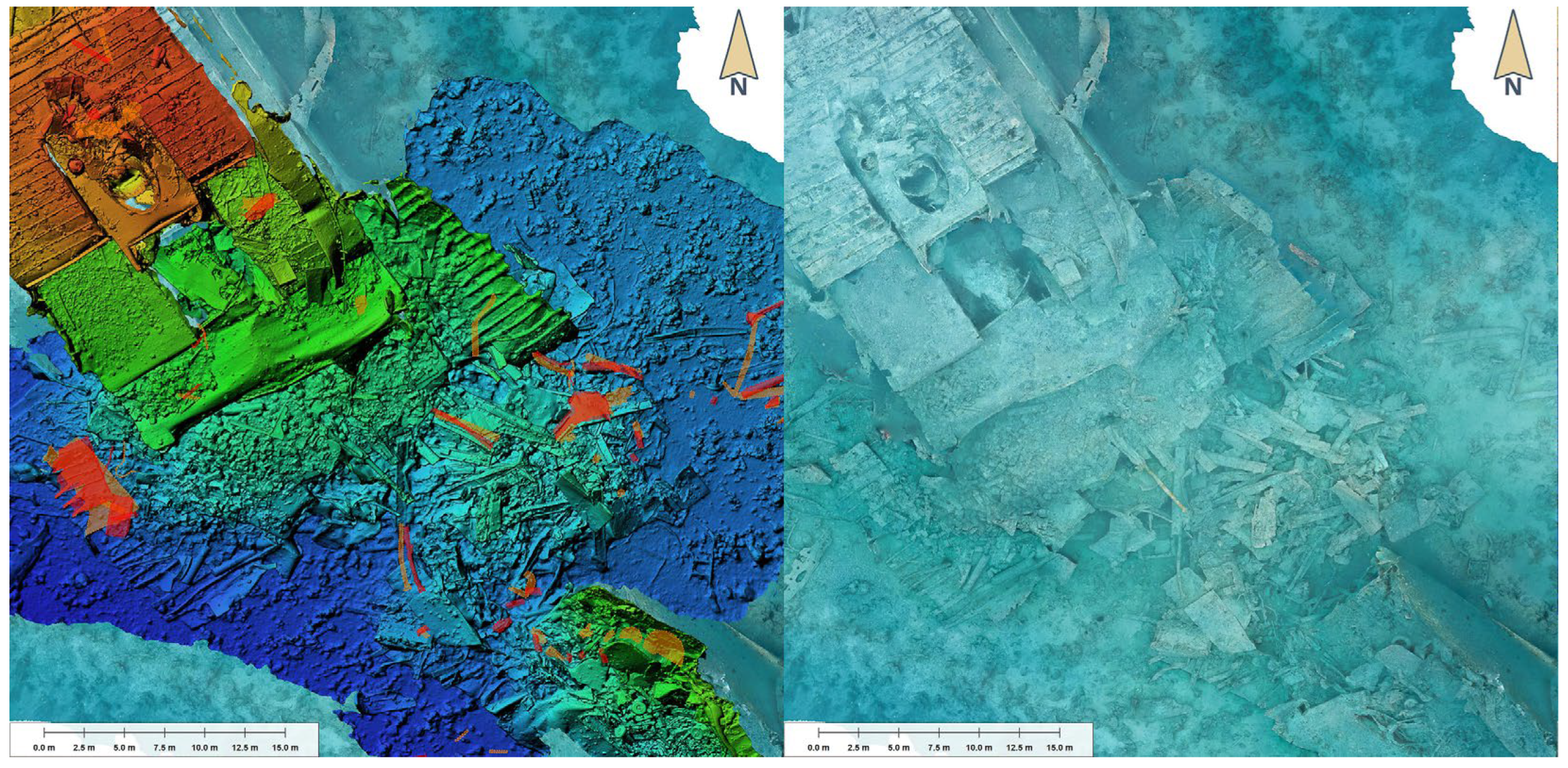
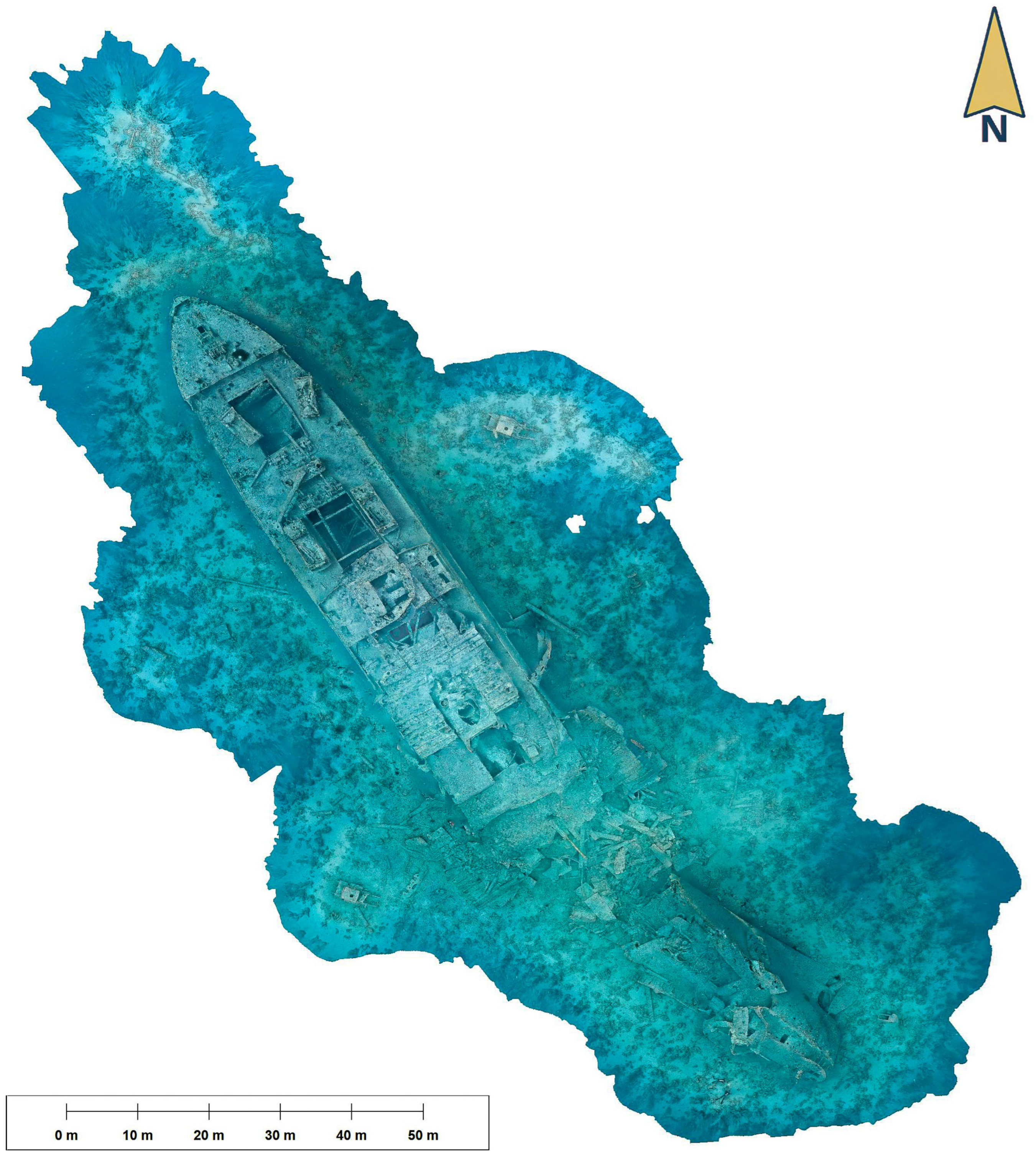
The 2022 season had two primary goals. The first was to record any changes to the ship’s structure and features since the last survey, including the location and presence of individual artifacts. This was performed to assess the impact of recreational diving on the site over time (Figure 10). Secondly, as we suspected the secondary explosion that sunk the ship had scattered remains over a large area of the seabed, we wanted to obtain an estimate of the extent of the debris field around the ship.

An additional 10,365 images were captured during the 2022 season over seven dives (357 min or 5 h 57 mins of in-water time). A total of 246 Gb of data was generated, and each image was tagged with a location and description before being processed in Agisoft Metashape Professional version 1.8.3 to validate the overlap and suitability for 3D reconstruction (see

Table 2. Summary of areas surveyed during the 2022 fieldwork, the area covered, purpose, and number of images.

Location	Area	New or Comparative	Number of Images
Port locomotive boiler	1874.5 m2	New	1980
Starboard locomotive boiler	1104 m2	New	1050
Starboard locomotive wheel	111 m2	New	137
Aft mast	1164 m2	New	1076
Hold No. 2 central debris field	536 m2	Comparative	678
Port anchor	484.8 m2	Comparative	641
Port engineer’s quarters	162.75 m2	New	242
Starboard engineer’s quarters	300.75 m2	New	426
Hold No. 4 debris field *	1848 m2	Comparative	809
Starboard machine gun mount	33.1 m2	Comparative	51
Hold No. 3 lower deck	987.8 m2	New	1209
Internal storeroom	151.8 m2	New	425
Stern anchor	N/A	New	74
Hold No. 1 upper deck collapse area	65.3 m2	New	290
Total new survey area /comparative	9184 m2/2901 m2		8662

). All areas were recorded using the same camera, lens, and lighting combination as used in 2017. The exception to this was the Hold No. 4 debris field (marked * in the table), which was recorded by Mohamed Salama using an Olympus TG5 rugged waterproof camera (Olympus Corp. Shinjuku-Ku, Japan) with an INON UWL-100 Wide Conversion Lens Type 2 (M67 Thread) (Inon Inc., Tokyo, Japan) and a Sea&Sea YS-01 strobe (Seas&Sea Co., Tokyo, Japan).

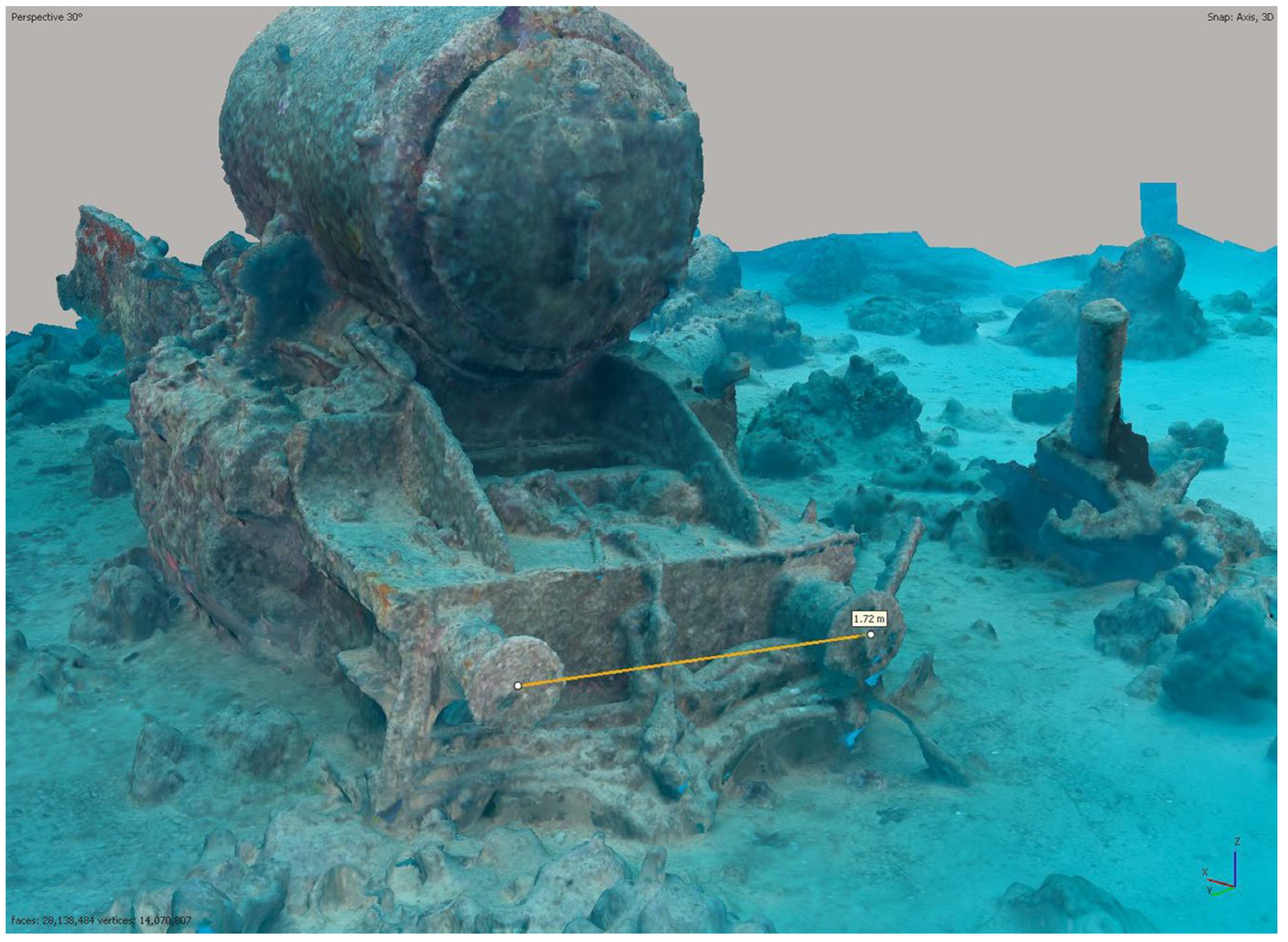
For smaller or more remote artifacts, local scaling to each model was applied using scale bars placed in each scene. For those objects close to the main wreck site, a series of image tracks were created to form a physical join between any artifacts on the surrounding seabed and the main wreck site surveyed in 2017. By carefully selecting a robust and existing feature (port locomotive smoke box, for example) with 2022 images overlapping the alignment to the main wreck site model, it may be accomplished by either using the Cameras or Markers chunk alignment method.

Comparative survey areas were selected based on three broad criteria. First, areas with known and clearly visible changes; second, areas considered at risk of structural deterioration; and third, evidence of disturbance or removal of items due to diver activity and/or looting.

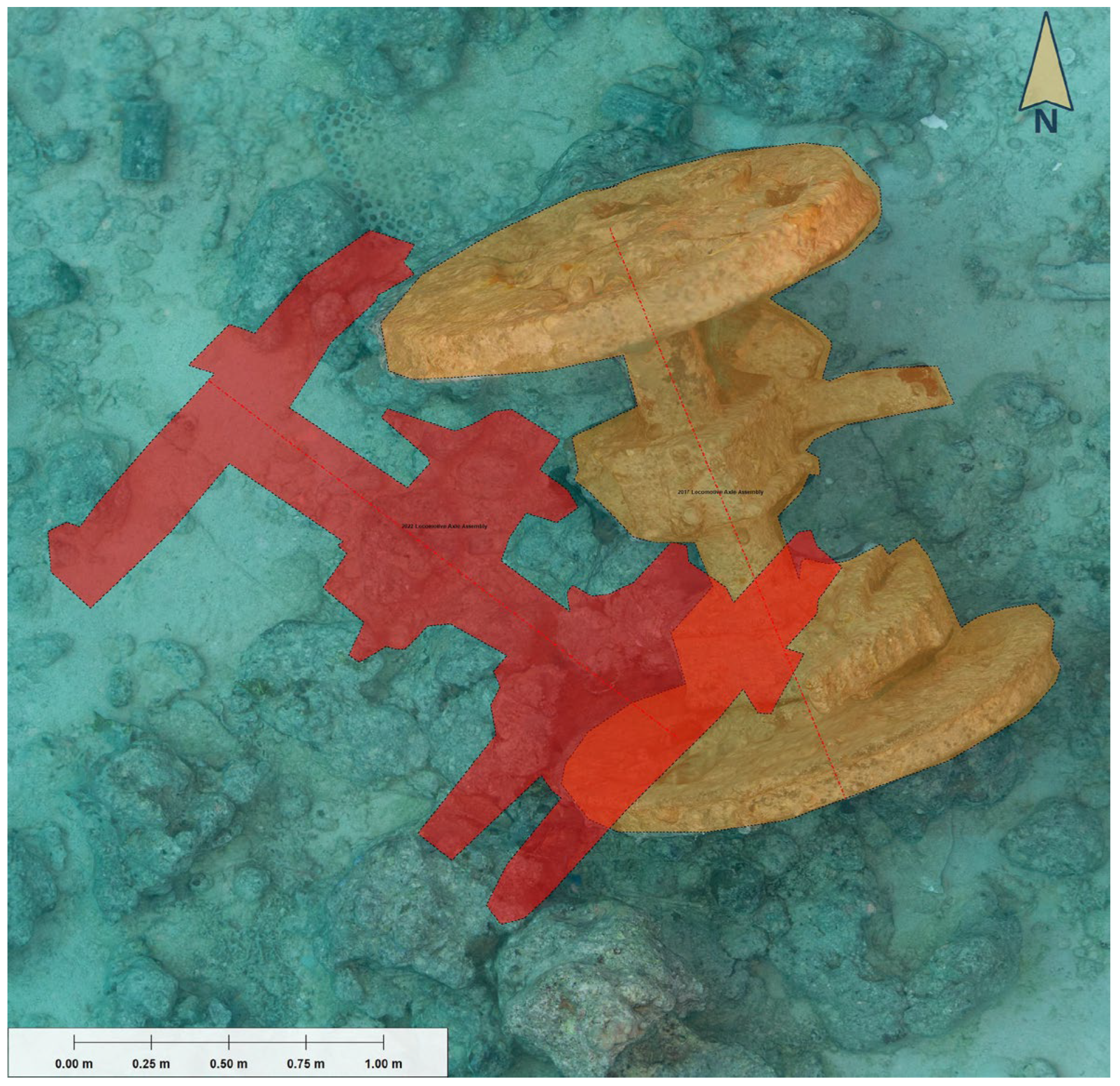
One issue arose during post-processing when using a substantial and believed-to-be static object. In order to align it with the main wreck, we selected a locomotive wheel assembly with an estimated mass of 2 tons, which was present in the 2017 survey. Given the minimal expected movement of the object between the surveys, it was considered a low-risk choice. However, during the post-processing alignment of the starboard boiler model, it became evident that the wheel assembly had rotated by 30 degrees at some point between the 2017 and 2022 surveys (Figure 11). The reasons for this movement are unknown, but it was most likely caused by a vessel mooring line. This unexpected movement of the wheel assembly resulted in excessive error when attempting to align the features of the assembly. Five alternative and common points from less-obvious features were chosen for alignment to correct the issue.

6. Post-Processing Methodology

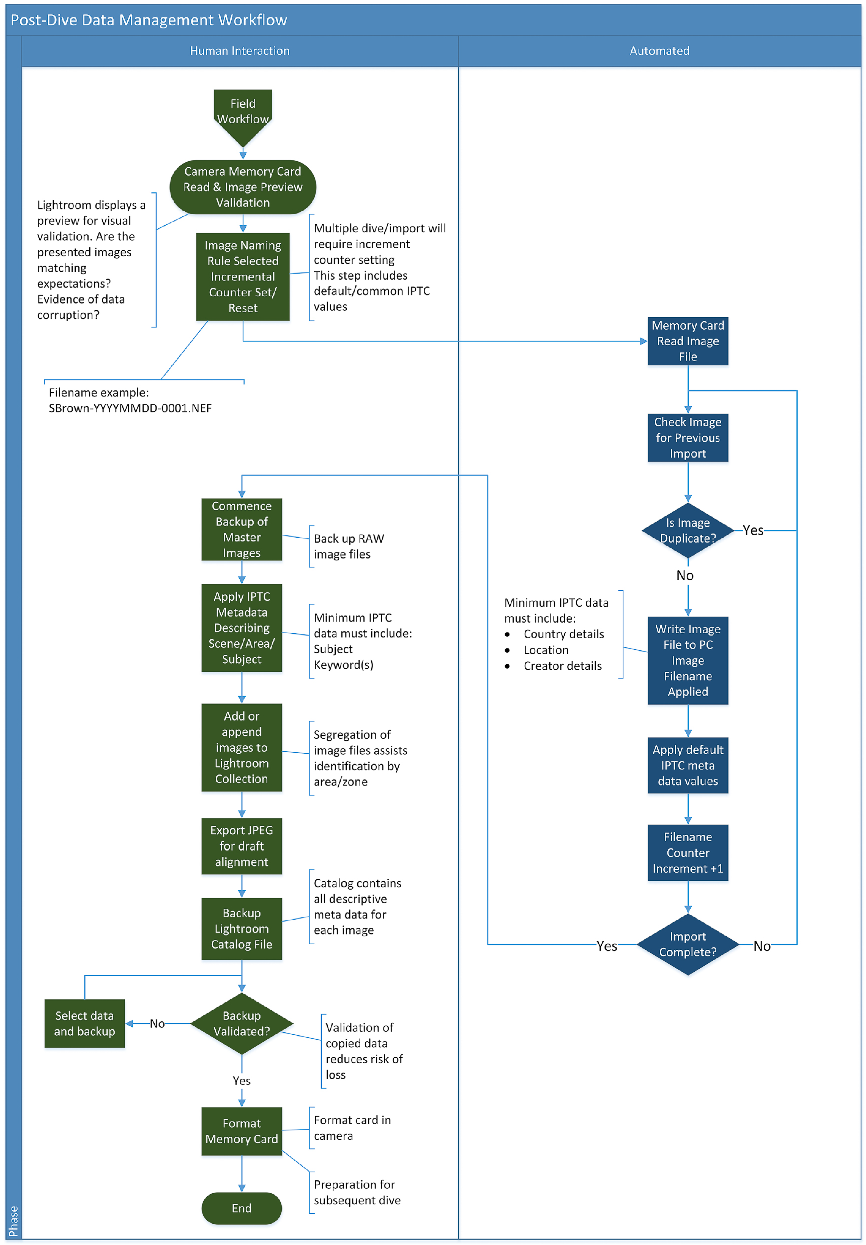
6.1. Data Management

Setting a clear data-management strategy in the field is one of the most important and often overlooked factors in executing an underwater photogrammetry project, especially when dealing with a large subject captured over multiple dives. Photogrammetry can quickly generate masses of unstructured, unordered data. Issues of image traceability and retrieval are compounded when more than one photographer is contributing to a project. As a result, a method for managing images is critical (Figure 12).

During the Thistlegorm survey, the following method was applied to every contributing image copied from the camera memory card:

• Each image carries a unique identifying filename. The point-of-capture filename assigned by the camera is discarded during the read/import process from the card to computer.

The following format was used: Name-YYYYMMDD-NNNN, where “Name” represents the name of the photographer/contributor (required for projects with more than one contributor, optional for single contributor work), and where:

YYYY represents the four-digit year of creation, e.g., 2022;

MM represents the two-digit month of creation, e.g., 05;

DD represents the two-digit day of creation, e.g., 25;

NNNN represents a 9999-digit sequential next number, e.g., 0001. This counter is reset to 0001 at the beginning of each day.

The dashes are included to assist human viewing and interrogation.

The use of the photographer/contributor name in the filename is duplicating data, as this information is held in machine readable IPTC field <creator> metadata field, but adding the creator name prevents filename collisions and potential data loss when working with multiple contributors.

An example would read:

SBrown-20220525-0001.NEF.

This is the first image taken by the author on 25 May 2022.

2.

The International Press Telecommunications Council (IPTC) metadata fields are automatically appended with the correct values as follows:

Creator information: creator, job title, address, city, state, postal code, country, phone, email.

Image information: sublocation, city, state, country/region, ISO country code.

Copyright information: copyright status, copyright.

Most of the above values are fixed and static during the project. Unchanging metadata such as this are applied as part of a preset.

3.

The changing metadata of title, caption and keywords are more volatile and depend on the area or region of the wreck. These fields were used to record the section or area of the ship the image relates to.

The value of this step and the information contained therein cannot be understated. The material gathered during the 2017 fieldwork has been retrieved and reprocessed at least twice. Without a means to isolate and identify a very specific set of images from over 24,000 images, the processing would either fail due to missing overlap, take prohibitively long to identify relevant images, or (most likely) not occur in the first place.

An example applied to keywords at import and subsequently used to identify and isolate 1980 images of the port locomotive remains are boiler, dive one, locomotive, port.

These keywords are enough to distinguish the images from the starboard boiler (which looks near-identical) and enable otherwise featureless images of the seabed to be related to the nearby feature of interest.

Keywords, titles, and captions should be applied immediately after the dive when the memory is fresh.

IPTC fields are machine-readable, transportable, and inherently embedded in the image file. For these reasons, they are considered a primary source of project data and value, and their use was mandatory.

4.

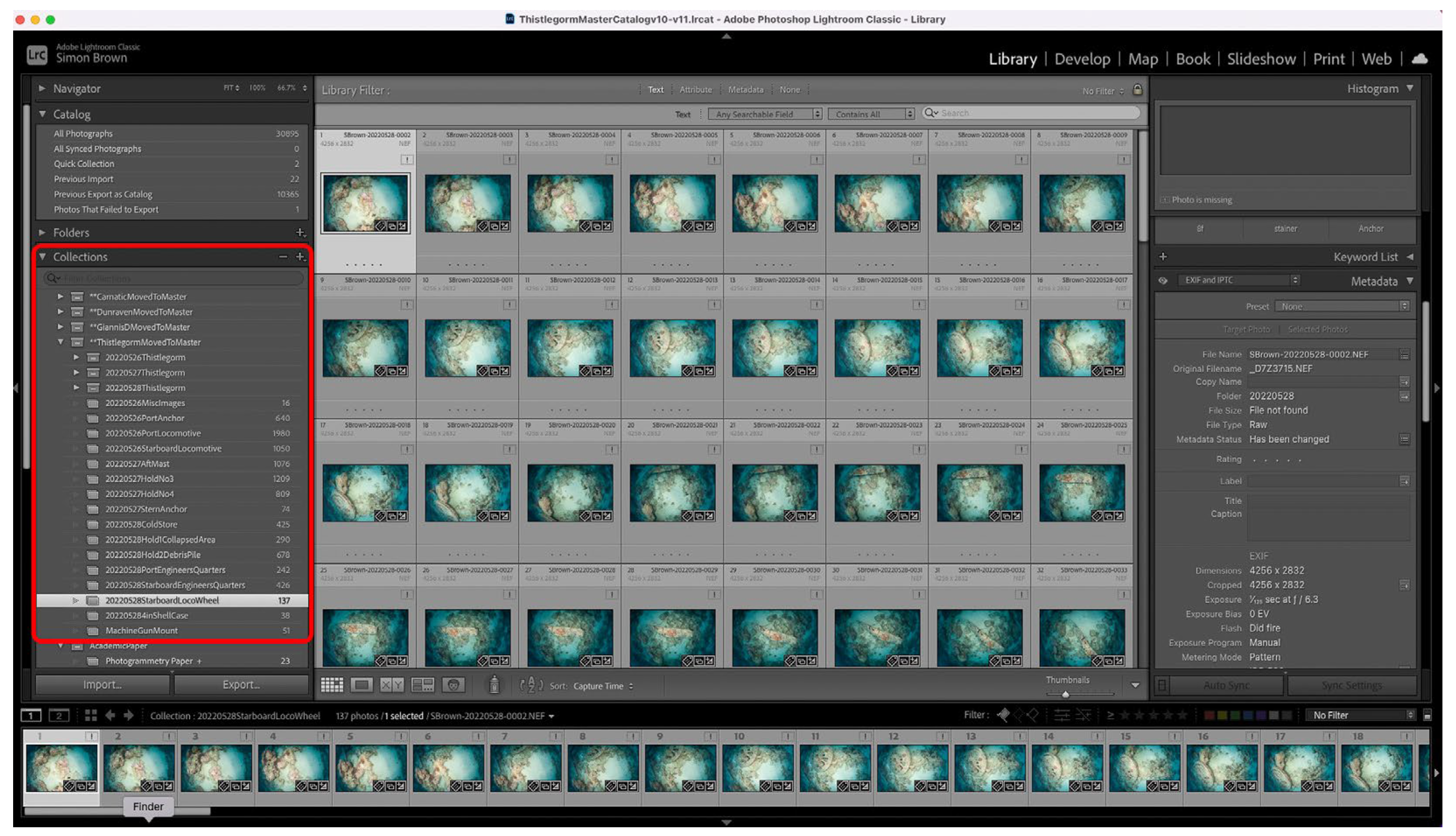
Further cataloging and segregation of data are applied using Adobe Lightroom Collections

For ease of use and quick access, relevant images are grouped into Lightroom Collections, enabling very fast retrieval of sets of relevant images (Figure 13). Adobe Lightroom Collections are generally not machine-readable, not transportable, and not inherently embedded in the image file. For these reasons, they are not considered a primary source of project data and value. That said, they are very convenient when working in Lightroom, and every subject covered on the various projects was afforded at least one Collection describing the group of related images.

6.2. Data Storage

Due to the large amount of image data captured on each dive, the organization and storage of these data are paramount (Figure 14). The segregation of RAW files into daily folders provides a logical and manageable break in data. At the beginning of each day, a folder would be created and named thus:

YYYYMMDD.

where YYYY represents the year of creation, MM represents the two-digit month of creation, and where DD represents the two-digit day of creation.

All dated folders were stored under a single parent folder residing on the laptop SSD. After successful copying and importing into Lightroom, both the RAW images and Lightroom catalog file were backed up to a separate 2 Tb SSD, with a minimum of two copies of these critical files existing at any one time.

At the end of each day, a second copy of all data was made to a second SSD. The backup of daily data is identified by the folder name named for the day where the images reside.

The importance of the information contained within the Lightroom catalog was (and remains) of extreme value, with loss of image metadata via accident, theft, data corruption, or hardware failure a risk to the project. Thus, the Lightroom catalog and RAW files were backed up together.

6.3. Data Processing—2017 Season

During the 2017 season, all images were shot and stored on the camera memory card in 14-bit Nikon NEF format. This format cannot be used directly by photogrammetry applications, so conversion to JPEG was performed using Adobe Lightroom. Image adjustments, such as exposure, contrast, clarity, vibrance, and saturation, were applied to enhance the visual appeal of the final model texture, but level changes were kept to a minimum. Ambient light levels permitted a low ISO value (typically ISO 400) and a high shutter speed (1/125th), thus negating the requirement to apply additional noise reduction during image preparation prior to export. No JPEG compression was applied during conversion from NEF to JPEG format, but image downsampling to reduce processing time from full-resolution 4286 × 2832 pixels to 3006 × 2000 pixels was applied when exporting the derived JPEG files.

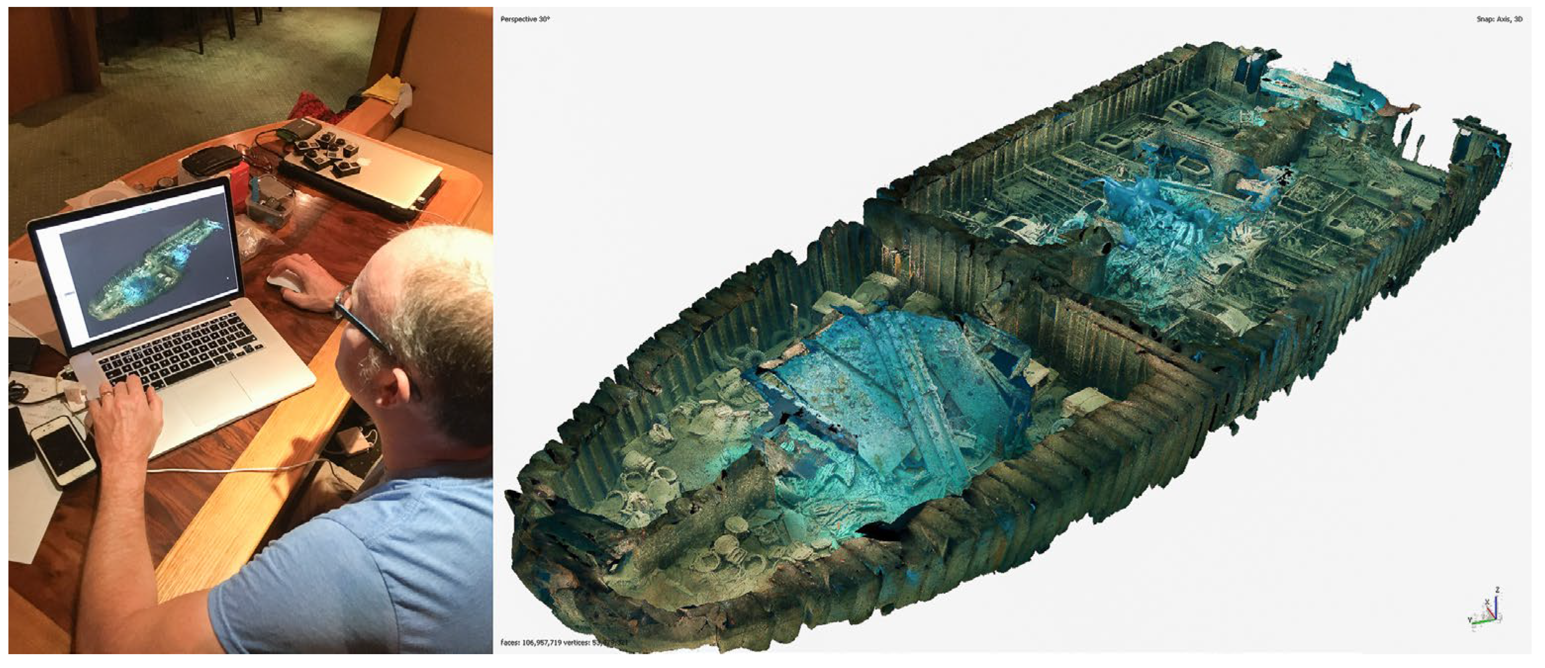
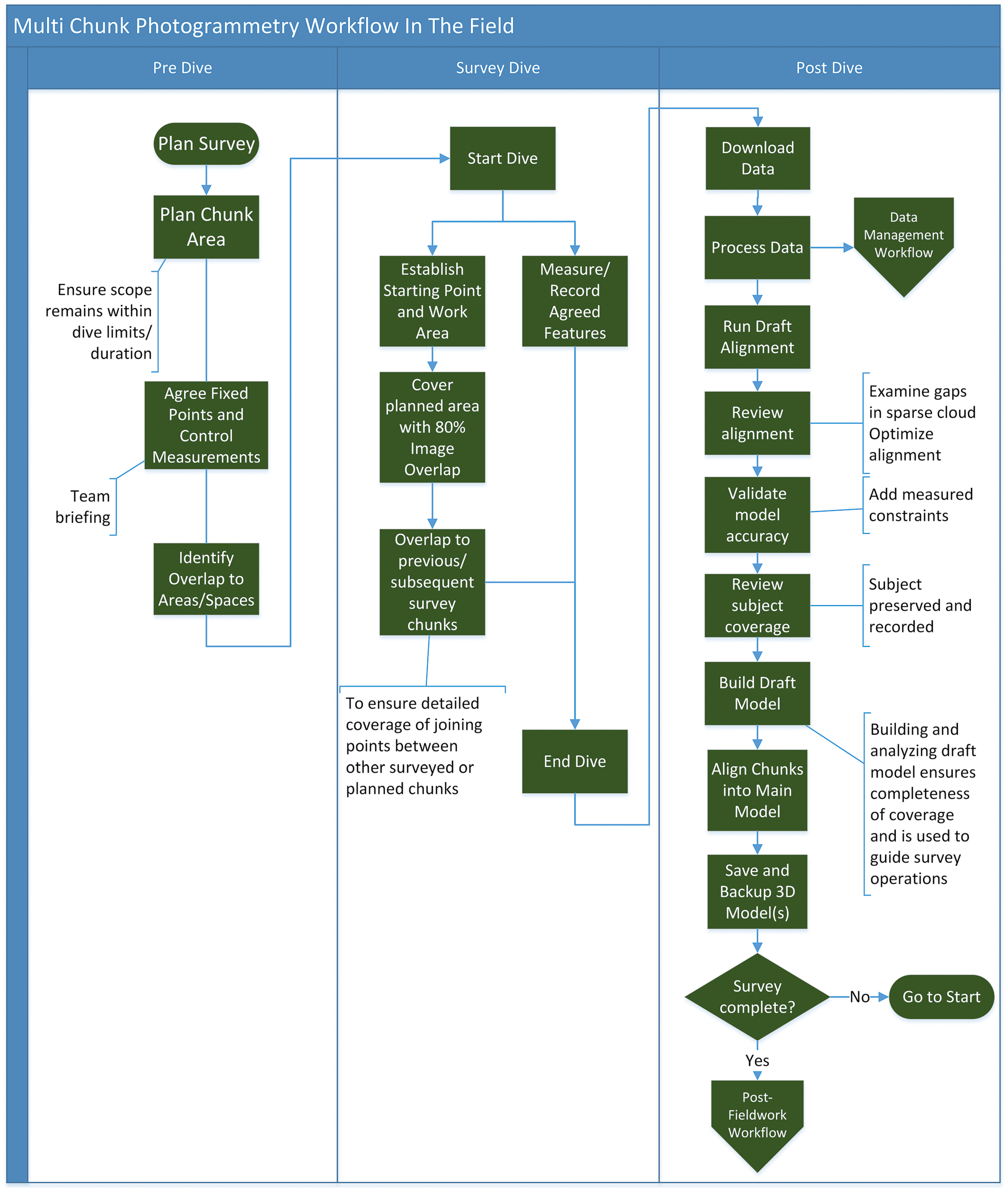
Processing the model began on-site using an Apple Mac Book Pro laptop running Agisoft Photoscan Pro V1.3. A draft model was assembled after each dive was completed (Figure 15). The draft model produced from downsampling from full resolution proved the images were aligning well and allowed direct recording of survey measurements. The draft model provided an invaluable reference for when the final model processing commenced.

Using a laptop is perfect for draft work and accuracy testing in the field, but the construction of final models demanded more resource, particularly in terms of RAM and Graphical Processing Unit (GPU) capacity (Figure 16). If available, GPU hardware processing is used at several stages of photogrammetric processing and reduces the time to simultaneously execute complex calculations required for 3D reconstruction. With a compact and lightweight design, laptops have limited RAM and lack a GPU, limiting the level of detail that could be processed in an acceptable timescale.

Early in the final build, the decision was made to use Amazon Web Services (cloud-based processing). Cloud-based computing offers a cost-effective and flexible means to access high-end computing, with the ability to switch specifications of the hardware (typically more RAM and more GPU processing) as the project dictates.

Using cloud services generated its own issues of bulk data transfer, but ultimately, processing in the cloud ensured the final model was built and ready.

The following workflow methods were applied to each section of the wreck:

• Align images: high settings with the key point (clusters of pixels recognized as potential matches to neighboring frames) limit set to 40,000 and tie point limit set to 4000 (maximum number of key points identified as matching others).
• Add scaling constraints and geo-location markers.
• Process outputs:

  a.

  Dense cloud: high setting.

  b.

  Mesh: source—dense cloud, surface type—arbitrary, and face count—high.

  c.

  Texture: size/count—8192.

  d.

  Ortho Photo: source mesh.

  e.

  DEM: source mesh.

It is important to note that the above workflow applies to Photoscan 1.3. Advances in the software add capability with greater efficiency and accuracy (see the 2022 processing section below).

For the main site, comprising just over 14,000 images, the available hardware could not process the model as one entity. A Metashape python script split_in_chunks.py (Github) was run, and the main model was sectioned into 15 (3 × 5) equal chunks. Each chunk was then processed separately before being merged back into a single chunk and 3D model.

Agisoft (authors of Photoscan Pro) kindly provided an additional time-limited license to enable concurrent processing both locally and in the cloud. After the 2017 fieldwork was complete, post-processing of the data took 45 days (1080 h) of local computing runtime, 23 days (556 h) of cloud computing runtime, and 68 (1636 h) days of continuous computer processing in total.

Whilst data were being processed, additional manual tasks were conducted: processing images, sorting data, reviewing model stages, uploading to the cloud, downloading from the cloud, backing up, organizing batch jobs, analysis and verification, etc.

In processing the images, the sparse cloud for the main wreck model of the SS Thistlegorm contained over 6 million calculated points, and the processed dense clouds of sections of the wreck had tens of millions of points. For example, the dense cloud for the lower deck has nearly 41 million points.

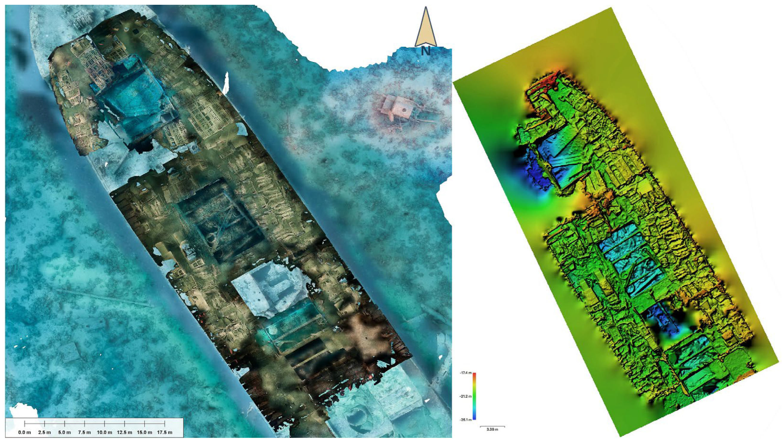
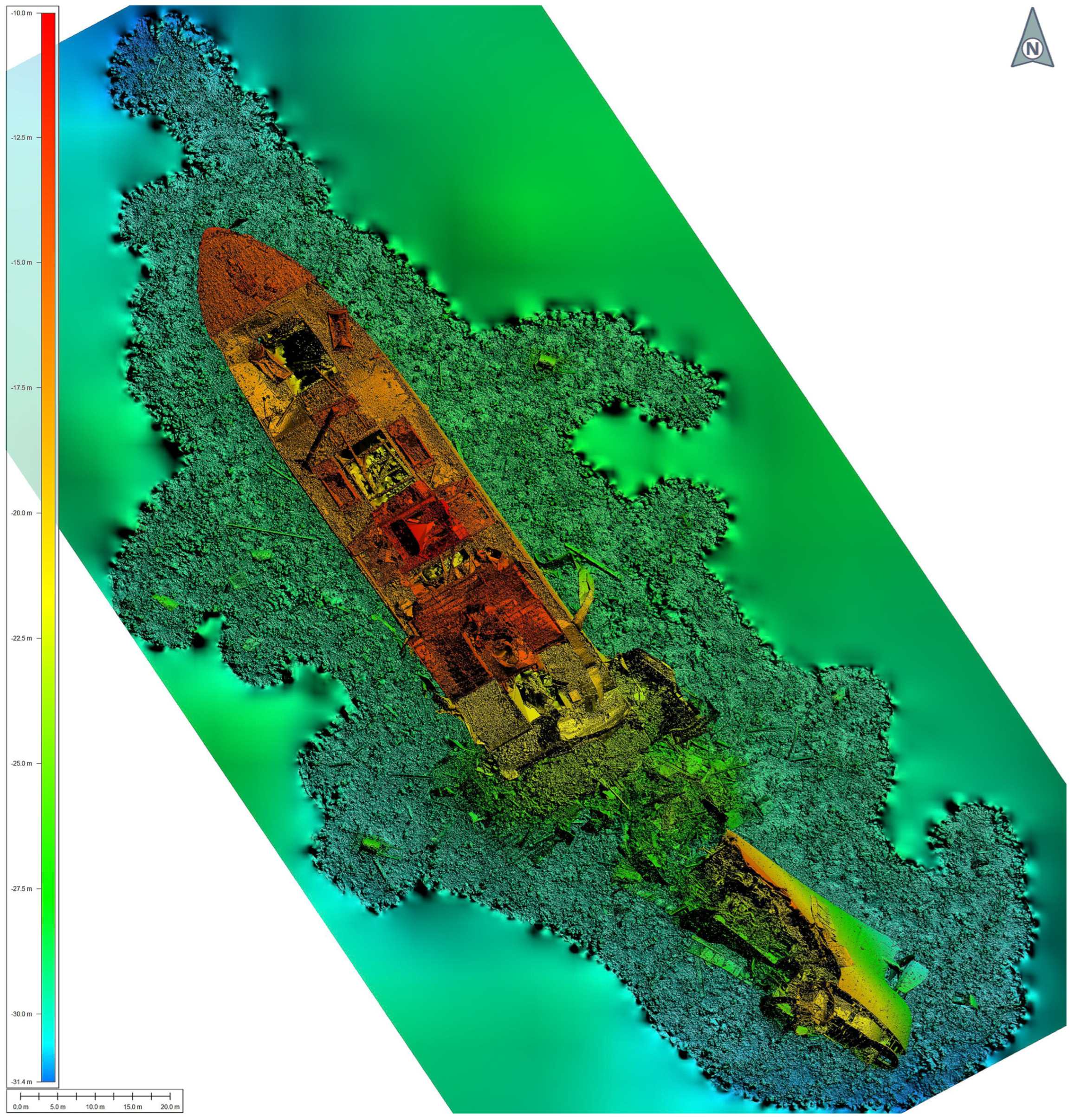
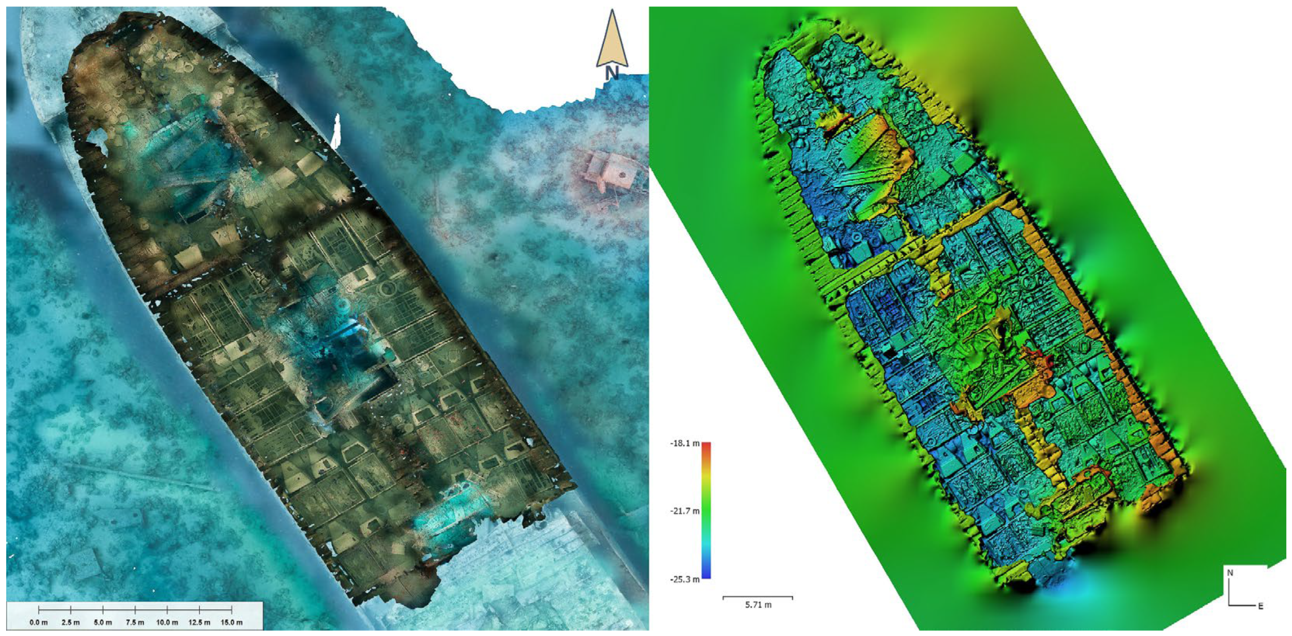
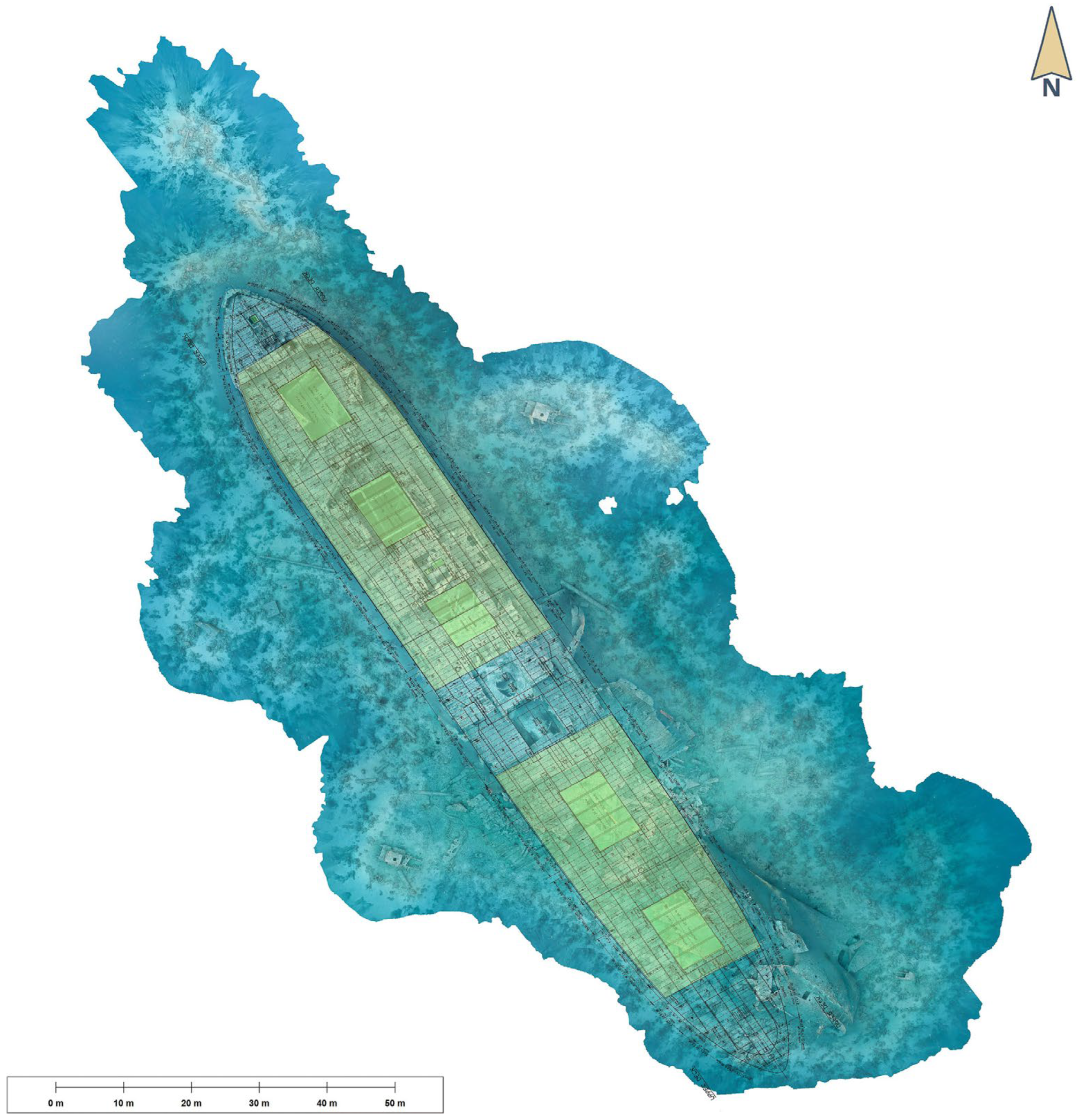
Two-dimensional orthophotos and digital elevation models (DEMs) can be extracted from the model to create geometrically accurate plan views (Figure 17). As measured points and GPS data were used during the build, the resulting image can be scaled and measured. With 14,000 high-resolution images, the main site orthophoto was generated at an accuracy of 10 mm per pixel (attempts to obtain higher resolution caused out-of-memory errors and crashed the hardware). With around 5000 or so images, the hold orthophotos were generated to an accuracy of 1 mm per pixel.

6.4. Data Processing—2022 Season

All images were processed on site using Apple MacBook Pro hardware (Cupertino, CA, USA), with Adobe Lightroom (San Jose, CA, USA) used to manage the images and metadata. Agisoft Metashape Professional v1.8.3 (St Petersburg, Russia) was used for rough draft 3D reconstruction and model/data validation prior to leaving the site. Image conversion from NEF to JPEG was again performed by Adobe Lightroom, with minimal color/tone/exposure value changes, devoid of noise reduction, and no compression applied. Due to advances in processing capacity, converted images were not downsampled, retaining a full level of detail. Upon return to the office, high-detail processing was carried out using a Mac Pro tower desktop with a 3.5 Ghz 8-core with 48 Gb RAM and Radeon Pro GPU alongside a PC with an Intel^® Core™ i9 16-Core Processor i9-12900KS (3.4 GHz) (Santa Clara, CA, USA), 128 Gb RAM, and NVIDIA GEFORCE RTX 3080 Ti GPU (Santa Clara, CA, USA) running Windows 10. This hardware had sufficient capacity to process each model as a single entity, including the main site, and the use of the split_in_chunks.py script was not required.

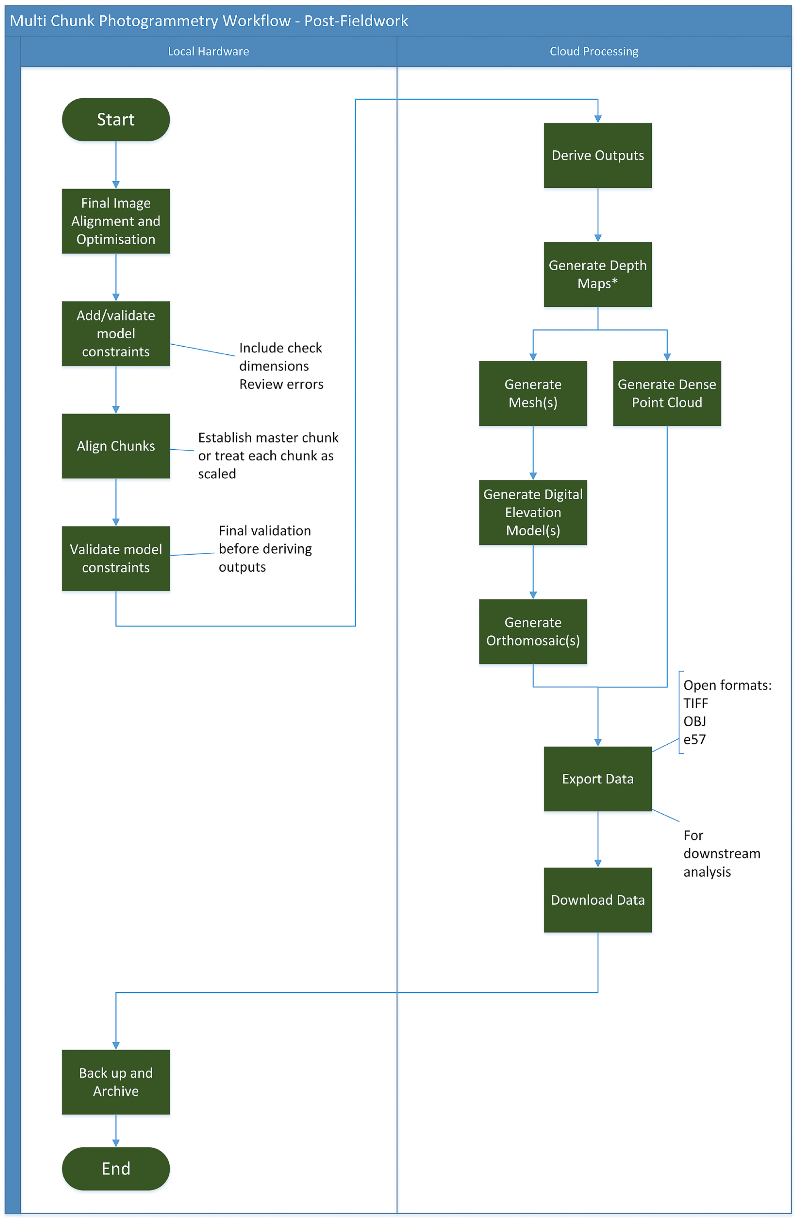
With advances in workflow knowledge, Metashape capability, and hardware capacity, the 2017 data were reprocessed, with each image exported at full resolution. A revised workflow was used to process (and reprocess) the data:

• Align images: high settings with keypoint limit set to 40,000 and tie point limit set to 4000.
• Recursive optimization: reduce error (pix) to <1 pixel and maintain tie points >100.
• Add scaling constraints and geo-location markers.
• Batch-process the outputs:

  a.

  Mesh: source depth maps. Surface type—arbitrary, face count—high, depth filtering—aggressive.

  b.

  Texture: size/count—8192.

  c.

  Ortho Photo: source depth maps.

  d.

  DEM: source depth maps.

Depth maps represent a very efficient alternative to using a dense cloud as a source for the mesh and subsequent outputs. In certain instances, and in recognition of the value, the DEM (step 4d) and the ortho mosaic (step 4c) were processed ahead of the mesh. For the 2022 work, the dense cloud was not required or processed.

6.5. Recursive Optimization of Aligned Images

The recursive optimization of camera alignment and removal of weak or inaccurate tie points between cameras, prior to the addition of scaling and geoconstraints, should be applied prior to generating the mesh, ortho mosaic, and digital elevation model.

Tie points, clusters of pixels recognized to match between overlapping images, are detected during alignment. The estimated accuracy of tie points is recorded by Metashape, and a summary of the total tie point variance is recorded. The objective of recursive optimization is to gradually remove inaccurate tie points and permit only those considered most accurate to constrain cameras with respect to their overlapping neighbors whilst preserving the maximum number of tie points per camera.

During the optimization process, the number of projections for any given camera should remain > 100 whilst aiming for a maximum pixel error of <1.0. Images exhibiting tie points < 100 or those with pixel errors > 1.0 should be examined manually.

Images with an uneven distribution of tie points, either clustered or with linear distribution, should be disabled and play no part in reconstruction as they may produce errors such as distortion in the outputs.

Recursive optimization is performed on the aligned cameras prior to adding distance or location constraints and prior to performing steps that generate the outputs, such as the mesh, DEM, or orthomosaic.

6.6. Accuracy Validation

As previously discussed, a network of measured control points was established during the fieldwork. This was used as the baseline for testing and scaling the photogrammetry work as it progressed. Metashape Professional permits the application of discreet and individual accuracy values on the following measured values:

• Latitude.
• Longitude.
• Altitude (depth).
• Scale bar constraints.

This enables each measurement to be assigned a confidence level and weighted by a tolerance value. GPS positions were considered low confidence and were assigned a tolerance of 5.0/5.0/0.3, respectively. Depth was measured using a diver’s computer and assigned a higher tolerance than GPS measurements. Distance values recorded by tape measure were assigned a medium level of confidence and assigned a tolerance of 0.25 m One diver-sourced measurement recorded an estimated error of 0.9 m and was not used during reconstruction. Distance values between coded targets on fixed scale bars were considered high confidence and assigned a tolerance of 0.001 m.

In 2019, a further dataset was obtained. The original builders’ plans were located in the Tyne and Wear archives, providing a rich source of information, including direct measurements, that could be applied to the data during the construction of 3D models of the wreck. Though some deviation from the plans might be expected due to the wreckage of the ship, identifiable features from the plans were used to validate the 2017 measurements, and these measurements were assigned an estimated error of 0.01 m The identification and dimensions of substantial artifacts and features identified in the original builders’ plans confirmed a high degree of confidence in the accuracy of the overall model (between 0.09% and 0.66% deviation from “as designed” to “as recorded”).

Additional measurements taken from the ship plans were subsequently used in the 2022 re-processing of the site data. Submitted for approval to Lloyds of London (and held in their historical archive), the plans are considered to be an accurate record of the as-built ship prior to sinking. This approach led to the identification of previously unidentified objects and their use in the validation of survey and model accuracy.

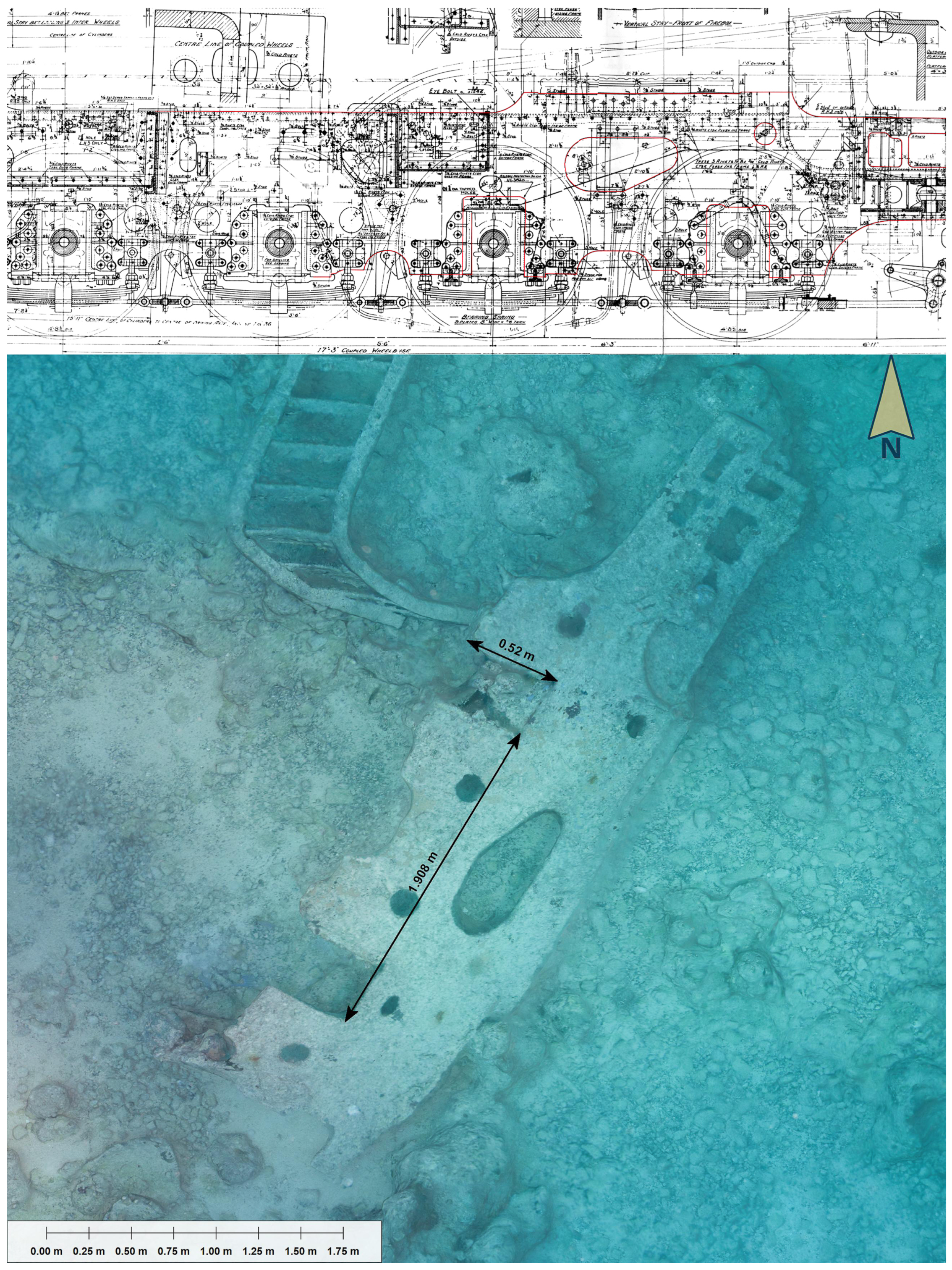
In 2019, a review of unknown but distinct objects close to Hold No. 4 revealed the existence of a very distinctly shaped section of steel plate. With proximity close to a railway locomotive and engine room, it was considered to be either part of the ship’s structure or part of a locomotive. A copy of the survey data of the plate was sent to the Stanier 8F Association, who identified it and sent back a marked engineering drawing of the locomotive showing the main frame profile matched the object (Figure 18). The engineering drawing included physical dimensions that documented the actual size of the object and permitted direct comparison to the orthophoto record. The distance between the centers of the two axles is recorded as 6′ 3″ or 1.9558 mm. When the distance is measured on the orthophoto, a value of 1.908 m is returned, a difference of 48 mm or 2.5%. The original manufacturing tolerances of this component are not known.

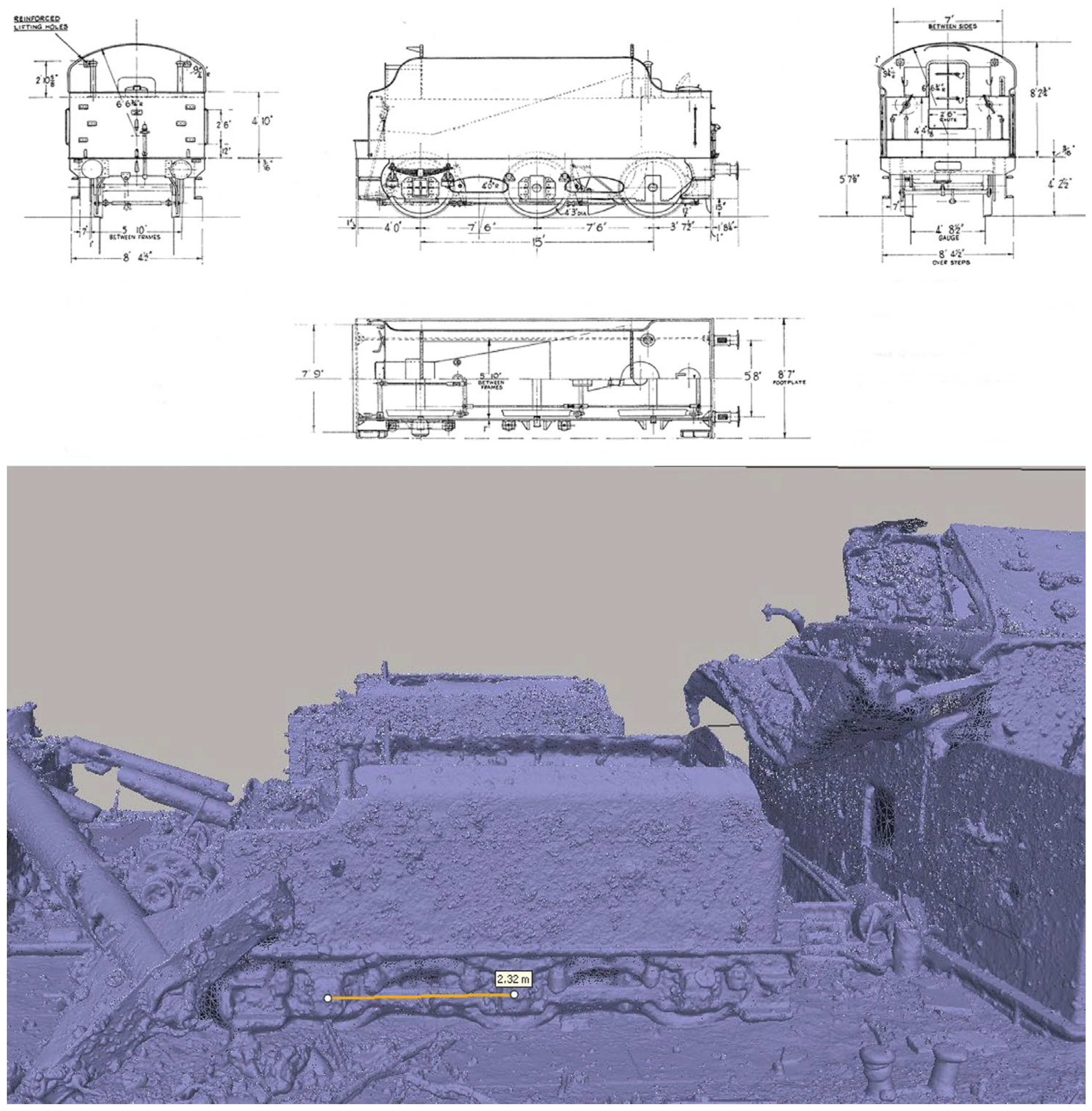
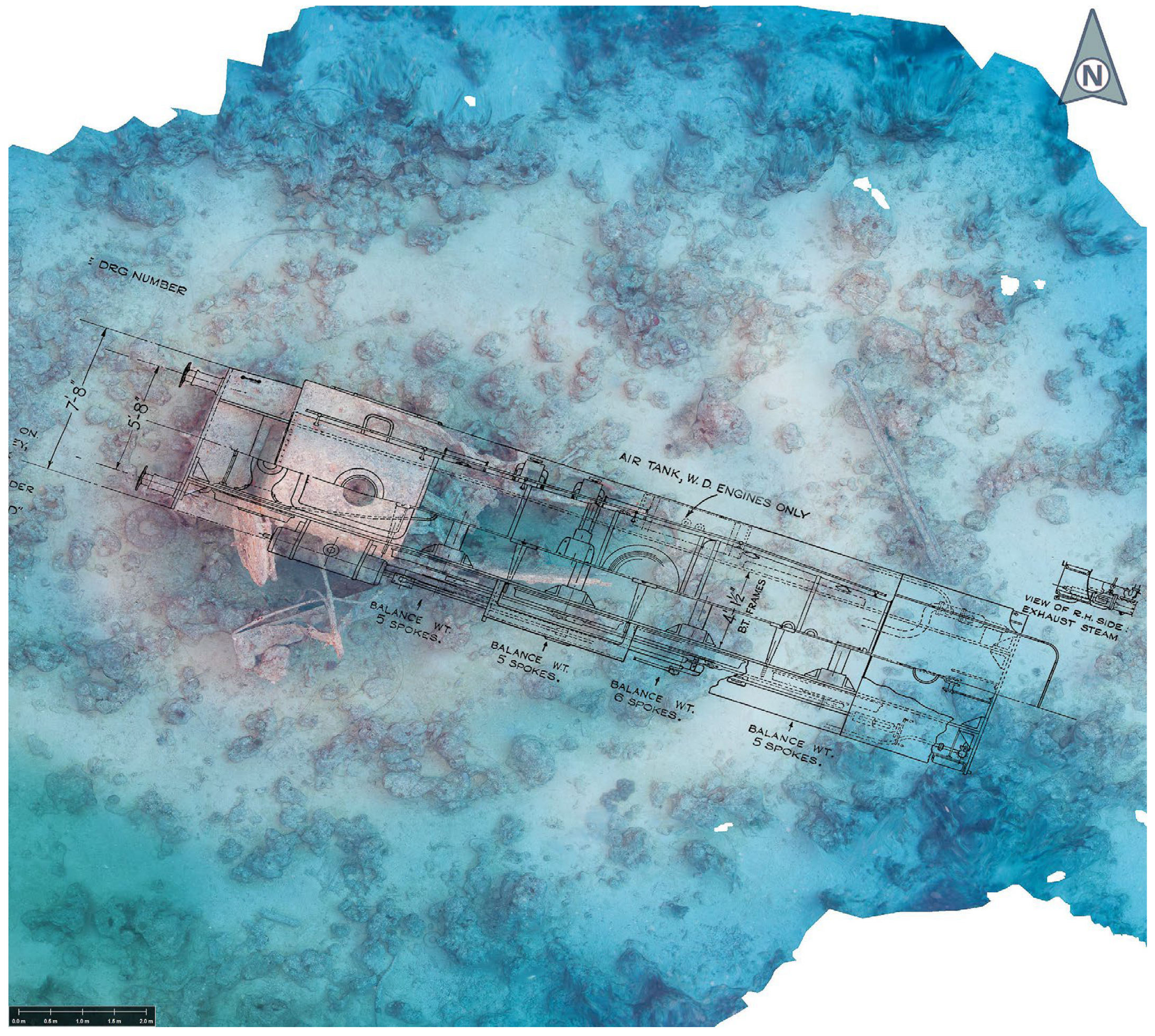
The presence of two locomotives and two fuel tenders has provided a rich source of model checking and validation, with both port and starboard smoke boxes being compared to contemporary engineering drawings (

Table 3. Measurement comparisons from the Stainer 8F steel plate, components, and fuel tenders.

Dimension	Engineering Drawing Value	Model Value	Variance
Stainer F steel plate—distance between axles	6′ 3″ (1.9558 m)	1.908 m	0.0478 m
Stainer F steel plate—pitch between cut holes	46″ (1.1684 m)	1.14 m	0.028 m
Strainer F plate—height of bearing block recess	20.5″ (0.5207 m)	0.52 m	0.0007 m
Distance between buffers of the starboard smoke box section of the Stanier 8F	5′ 8″ (1.7272 m)	1.73 m	−0.0028 m
The overall distance between outer frames of the starboard smoke box section of the Stanier 8F	7′ 8″ (2.322 m)	2.37 m	−0.048 m
The overall distance between main frames of the port smoke box section of the Stanier 8F	4′ 1.5″ (1.2573 m)	1.25 m	0.0073
The distance between buffers of the port smoke box section of the Stanier 8F	5′ 8″ (1.7272 m)	1.72 m	0.0072 m
The overall distance between outer frames of the port smoke box section of the Stanier 8F	7′ 8″ (2.322 m)	2.35 m	−0.028
The overall distance between leading and first driven wheel of the port smoke box section of the Stanier 8F	8′ 9″ (2.667 m)	2.67 m	−0.003
Measurement between rear and center axle centers of the fuel tender	7′ 6″ (2.286 m)	2.32 m	−0.034 m
Distance between buffer centers of the fuel tender	5′ 8″ (1.727 m)	1.74 m	−0.013 m
Distance between axle centers of the fuel tender	15′ (4.572 m)	4.64 m	−0.068 m

). The locomotives themselves were close to the secondary explosion that sank the ship and have been distributed in component form on the seabed [16]. However, the fuel tenders stowed alongside the entrance of Hold No. 2 are undamaged, and a selection of contemporary measurements can be validated by measuring directly from the 3D model. The variance between the values measured from the models is within a tolerance of 0.5~1.5% when compared to the as-built records of the fuel tenders (Figure 19, Figure 20 and Figure 21).

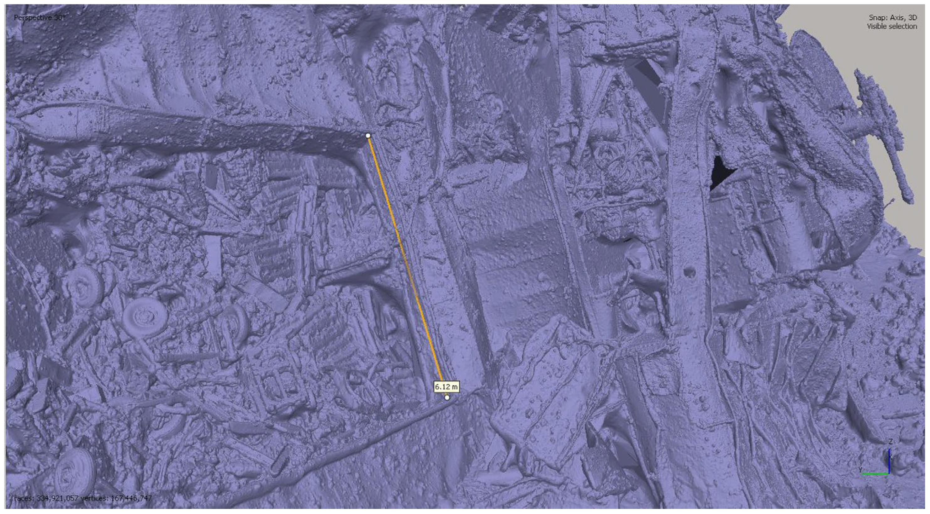
Due to the nature of the damage inflicted on the ship from the original explosion, it was not possible to apply any of the builders’ plan measurements to any point of the wreck beyond the entrance to Hold No. 3 and the aft surviving section of Hold No. 5. Areas of the main wreck retaining structural integrity could, however, be compared with the builders’ plans. For example, the aft end of Hold No. 5 measures 36′ 6″ × 20′ 0″ (11.1252 m × 6.096 m) on the building plans, and direct measurement from the model records the width of the hold today as 6.13 m, or a 0.66% variation from the shipbuilders’ intent (Figure 22). Although close to the source of the secondary explosion that sank the ship, the hold seems to have suffered little structural distortion.

6.7. Model Alignment

Aligning disparate 3D data, created 5 years apart, creates its own issues and considerations to ensure the two sets of models can be aligned.

Recorded in 2022, the store room, Hold No. 2 debris pile, port anchor 36, Hold No. 3, and both locomotive boilers were aligned with the main wreck model. Merging and aligning the models used three methods:

• Including 2017 and 2022 image datasets into a single aligned model.
• Using markers manually placed at common points between two models.
• Aligning additional 2022 images into the 2017 alignment and using common camera location to align.

Each method has benefits and disadvantages, typically with ease and speed of alignment providing compromise over absolute accuracy. Method 2, using human judgment to place markers in common locations, is the least accurate. Misalignment by a few pixels on each image can lead to compound errors over longer distances, such as those found on the upper and lower cargo decks.

The preferred methods are, therefore, 1 and 3, with the acceptance reprocessing entire datasets, which was applied to Hold No. 1 and 2 lower decks, and the addition of Hold No. 3 images may be required.

One subject photogrammetry cannot record is moving subjects. When choosing fixed and existing references known to be present in the 2017 data, care was taken to select only the most substantive, robust, and ultimately heavy objects, those least likely to have moved.

The port locomotive smoke box was considered a suitable reference, and this proved to be the case with the locomotive boiler model alignment.

The port locomotive railway wheels, mounted on a common axle complete with leaf springs, were judged to be of sufficient mass to have remained static and fixed, and included a fixed reference for the starboard boiler model. As previously discussed, the locomotive axle assembly was later shown to have moved between 2017 and 2022. Five alternative common points were used for alignment.

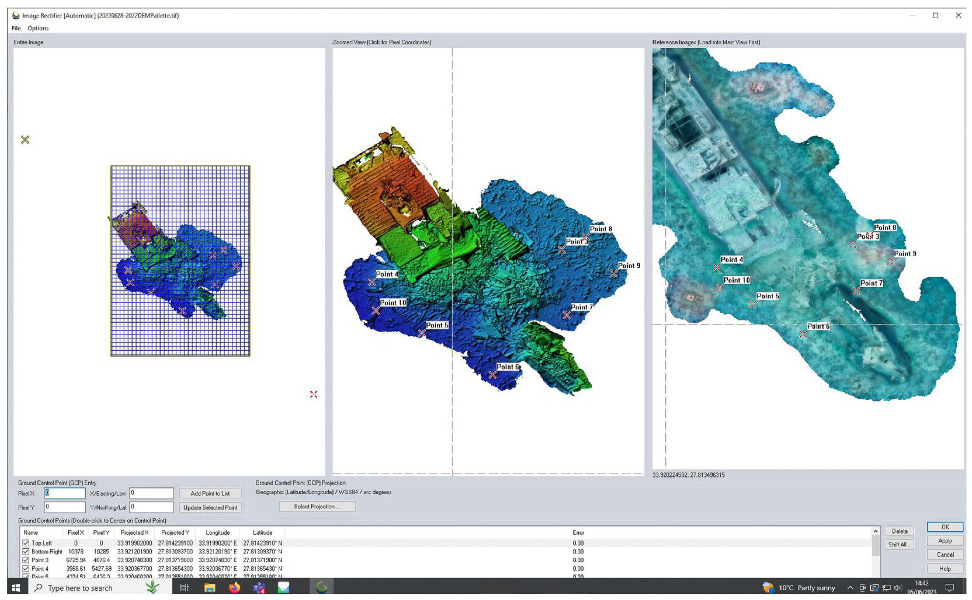
6.8. Manual Rectification and Public Engagement

Datasets processed and lacking scale or geo-reference location data can be used for comparative analysis and identification of change. Using the GIS software application Global Mapper Pro v24.1.0 (Blue Marble Geographics, Hallowell, Maine, USA), successive layers of 2022 data were added and manually rectified to align with the 2017 baseline orthomosaics (Figure 23). Care must be taken during manual rectification and requires an absolute minimum of 3 points to achieve a rudimentary orientated alignment. A greater number of points is advised, with 5 being the recommended minimum. Points should be evenly distributed and avoid referencing any feature at risk of movement. This approach has permitted the use of data that may otherwise have to have been set aside. Having a baseline othomosiac survey also allows the use of photographic images and data taken by recreational divers with differing levels of skill to record changes to the wreck over time.

7. Conclusions

The fieldwork and subsequent processing of the Thistlegorm have demonstrated the feasibility of conducting highly accurate 3D surveys of both the interior and exterior of intricate wrecks using off-the-shelf equipment at a low cost and with efficiency. Critical to achieving this accuracy is the capture of high-resolution images suitable for photogrammetric reconstruction, coupled with effective and efficient management of image data from the project’s outset. Establishing a clear post-processing workflow allows for the integration of additional data into the model once the geo-referenced baseline survey is established. The accuracy achieved by this project and the methods applied can be broadly broken down into two types. Firstly, the georeferenced data gathered using consumer (as opposed to survey)-grade equipment is likely to yield positional accuracy of ±5~10 m. For this reason, these constraint values were given low or weak weighting in the 3D model. Clearly, returning with survey-grade equipment is highly desirable but will remain difficult, with security levels in the Sinai likely to remain challenging for the foreseeable future. Secondly, the use of higher weighted constraints to scale the model locally has ensured that internal feature-to-feature measurements have been within ±1~2% of real-world distances. This method, of using weak GPS data combined with accurate local constraints, has delivered a 3D model that is approximately geolocated but features a very accurate and confident reconstruction. As a result, this dataset facilitates continuous monitoring of the Thistlegorm, not only during return visits but also as we receive images from recreational divers. The 2D and 3D outputs from the fieldwork have been made available online (http://thethistlegormproject.com) and have served various purposes, including aiding diving groups in pre-dive planning, engaging school groups in Egypt and the UK, and supporting professional bodies like the Tyne and Wear Museum (Figure 24). To date, the main site model on the Thistlegorm website, where divers are encouraged to contribute their images and videos, has garnered over 41,000 views. The published models have provided a substantial body of evidence not only supporting ongoing research into the wreck’s history and contents but also enabling the tracking of changes in the preservation of its remains over time.