Article

Surface and Underwater Acoustic Source Recognition Using Multi-Channel Joint Detection Method Based on Machine Learning

College of Meteorology and Oceanography, National University of Defense Technology, Changsha 410073, China
*
Authors to whom correspondence should be addressed.
J. Mar. Sci. Eng. 2023, 11(8), 1587; https://doi.org/10.3390/jmse11081587
Submission received: 24 July 2023 / Revised: 9 August 2023 / Accepted: 12 August 2023 / Published: 13 August 2023
(This article belongs to the Section Ocean Engineering)

Abstract

:
Sound source recognition is a very important application of passive sonar. How to distinguish between surface and underwater acoustic sources has always been a challenge. Due to the mixing of underwater target radiated noise and marine environmental noise, especially in shallow water environments where multipath effects exist, it is difficult to distinguish them. To solve the surface and underwater acoustic source recognition problem, this paper proposes a multi-channel joint detection method based on machine learning. First, the simulation data are generated using the normal model KRAKEN setting in the same environment as the SACLANT 1993 experiment, which uses a vertical linear array of 48 hydrophones. Secondly, the GBDT classifier and LightGBM classifier are trained separately, and then the model is evaluated using precision, recall, F1, and accuracy. Finally, four ML models (kNN, random subspace kNN, GBDT, and LightGBM) are used to analyze all 48 channels of hydrophone data. For each model, two kinds of feature extraction methods (module features, real and imaginary features) are applied. Generally, the results show that both GBDT and LightGBM models have better performance than both kNN and random subspace kNN ones. For both GBDT and LightGBM models, the results using module features have better performance than using real and imaginary features.

1. Introduction

Sound source recognition is a very important application of passive sonar. How to distinguish between surface and underwater sound sources has always been a challenge [1,2]. Due to the existence of a large amount of environmental noise in the ocean, especially in the shallow sea environment, the multipath effect of sound line propagation makes it difficult to deal with.
Various recognition methods have been proposed, but none of them has achieved the expected results. Direct estimation of source depth is a common method to solve this problem. As a traditional method for estimating source position and depth, matched field processing (MFP) [3,4,5,6,7,8] is realized by matching the measured pressure field with the copied pressure field. Accurate prior environmental information and an appropriate propagation model are the premise of constructing a replica pressure field. However, due to the spatiotemporal transformation characteristics of the ocean, the acquisition of environmental information is prone to bias, resulting in environmental mismatch and ultimately significantly degrading the accuracy of MFP.
In addition to MFP, there are some methods [9,10,11] used in underwater target localization. In 2017, Natalia et al. [9] discussed the issues of mechanically scanned imaging sonar (MSIS) imaging and the generation of artificial seabed model-based equivalents for the purposes of MSIS positioning. In 2017, Pawel et al. [11] proposed a passive detection algorithm for mobile ships in marine environments based on digital signal processors. In 2021, Witold et al. [10] used forward looking sonar for underwater target tracking.
Due to the difficulty of accurately estimating the depth of sound sources, rephrasing this issue as a binary classification for surface and underwater (S/U) acoustic source recognition has been considered [1]. In fact, mode trapping is a more classical method to distinguish S/U acoustic sources [12]. The approach is based on the recognition of gross differences in measured [13] mode spectrum shape between surface and submerged source classes induced by mode trapping [12]. Some work [12,14,15,16,17,18,19] has already implemented binary classification problems. Premus et al. [14] proposed a matching subspace method in 2007, which is suitable for shallow water waveguide depth identification. The experimental results show that the matched subspace formalism was able to improve recognition performance by removing subspace overlap imposed by aperture limitations. In 2013, Premus et al. [12] used the horizontal linear array (HLA) to identify sound sources with depths of 9 and 60 m based on the mode subspace projection method. Yang [15] demonstrated a data-based matching pattern source localization method in 2014. This method is used for moving sources and can use directly estimated mode wavenumbers and depth functions from the data. In 2016, Du et al. [16] used only two hydrophones to realize passive sound source depth recognition in shallow water environments. They proposed a new method of source depth recognition that uses the local angle of the interference striations directly from the LOFAR diagram with the help of two-dimensional discrete Fourier transform. In 2017, Conan [18] achieved source depth identification using the captured energy ratio based on HLA. The experiment successfully identified the surface combatant and the underwater towing source. In 2018, Liang et al. [19] used an HLA of acoustic vector sensors based on mode extraction for deep recognition of low-frequency acoustic sources. The constructed testing hypotheses are highly robust against mismatched environments.
In recent years, the deviation of underwater sound source ranging based on the machine learning method [20,21] is less than that of the traditional MFP method [5,6,8]. Relevant research shows that the machine learning model trained with observation data sets performs well in ship distance positioning. However, due to the difficulty of ocean observation, it is not practical to obtain all acoustic data for each source location (i.e., depth and distance) in a vast ocean area. Even though large amounts of data can be acquired by the automatic identification system (AISs), there is still insufficient training in database-supported models.
In machine learning (ML), surface and underwater source recognition assigns a label to a given input value. This is a typical binary classification problem where each input receives a value from the binary class. The recognition system is trained according to the marked “training” data in the case of supervised learning. When applied to S/U target classification, machine learning serves as an alternative tool to assign labels to input values. Machine learning methods do not require the establishment of physical models [1]. Machine learning methods directly obtain understandable information from data. In 2022, Wen Zhang et al. [1] adopted three supervised ML models: k-nearest neighbor (kNN), random subspace kNN (RS-kNN), and ResNet-18, using only one hydrophone to distinguish an S/U acoustic source. The results indicate that even with only one hydrophone, machine learning is feasible as a method for S/U acoustic source recognition.
In this paper, ML is also used in order to achieve better S/U acoustic source recognition. The training data are generated using KRAKEN and the environmental parameters of KRAKEN are the same as those in the SACLANT 1993 experiment, whereas the test data are actual sea trial data. This article adopts two classic machine learning methods, gradient-boosting decision tree (GBDT) [22] and light gradient-boosting machine (LightGBM) [23].
This article consists of six parts. Section 2 introduces the overall architecture of the article. Section 3 introduces two ML classifiers (GBDT and LightGBM). In Section 4, the simulation environment based on the experimental environment is established and simulation data are generated. In Section 5, the GBDT and LightGBM models are first trained and then evaluated using accuracy, recall, F1, and accuracy scores. Secondly, the trained models are used to analyze the experimental data of all 48 hydrophones of the vertical linear array (VLA). Thirdly, the results are compared among GBDT, LightGBM, kNN, and RS-kNN [1]. Finally, a summary and discussion are conducted in Section 6.

2. Overall Architecture [1]

The overall architecture of this article is shown in Figure 1. It mainly includes the following six parts: (1) setting the underwater acoustic environment. As a benchmark experiment for source localization based on MFP, the experimental data of SACLANT 1993 can be publicly accessed online [24]. The underwater acoustic environment is set up based on the SACLANT 1993 experimental environment. Section 4.1 provides a detailed introduction to the environmental settings. (2) Using KRAKEN to simulate S/U acoustic source signals received by a single hydrophone of all 48 channels. The simulation process is detailed in Section 4.2. (3) Data preprocessing. This part consists of two parts: feature extraction and data normalization. Feature extraction is to convert complex values into real values. Data normalization refers to limiting the preprocessed data to a certain range (such as [−1, 1]). The preprocessing can be found in Section 4.2, Section 4.3, and Section 4.4. (4) Training models using GBDT and LightGBM classifiers separately, as detailed in Section 5.1 and Section 5.2. (5) Testing the training model using the experimental data from SACLANT 1993, as detailed in Section 5.1 and Section 5.2. (6) Finally, multi-channel joint detection and results comparison among GBDT, LightGBM, kNN, and RS-kNN are shown in Section 5.3.

3. Theory and Method

3.1. KRAKEN [13]

The KRAKEN program is a sound propagation calculation software based on the theory of normal modes and is a part of the modeling tool in the ocean acoustics toolbox. It was jointly developed by the U.S. Naval Ocean System Center (NOSC) and the United States Naval Research Laboratory (NRL). After testing it in eight different marine environments and comparing it with real data, the model proved to be correct and effective.
Under the condition of layered media, the solution of the normal mode equation is a complex eigenvalue problem. The KRAKEN normal mode model uses finite difference methods to solve the normal mode equation, which can obtain fast and accurate solutions. It divides the entire seawater depth D into N equally spaced widths, h = D / N , and correspondingly obtains N + 1 points. By using the finite difference approximation, the continuity problem of the normal mode equation can be reduced to the eigenvalue problem in linear algebra. The solution of the wave pressure field can be obtained by using the KRAKEN method according to the adiabatic hypothesis and WKB approximation:
p r , z = i ρ ( z s ) 8 π r e i π / 4 m = 1 ψ m ( z s ) ψ m ( z ) e i k m r k m
where r is the horizontal distance; z is the depth; ρ represents the seawater density; z s represents the source depth; s = 0 , 1 , , N ; ψ m and k m are the obtained m-th eigenvector and eigenvalue, respectively; and m = 1 ,   2 ,   , .
Therefore, the simulation data generated based on KRAKEN is the numerical exact solution of the real data. However, compared to real experimental data, the simulation data have no noise.

3.2. GBDT [22]

GBDT is short for gradient-boosting decision tree. During training, a forward distribution algorithm is used for greedy learning. Each iteration learns a classification and regression tree (CART) to fit the residual between the predicted results of the previous tree and the true value of the training sample. GBDT pays attention to the residuals of the output in each training round. In the next round, the residuals of the current round are used as input to fit the residuals so that the residuals of the output in the next round will be smaller. Therefore, GBDT can change the gradient direction with a certain decrease in the loss function in each turn.
The idea of the GBDT binary classification algorithm is to use a series of gradient lifting trees to fit this logarithmic probability, and its classification model can be expressed as:
P Y = 1 x = 1 1 + e F M ( x )
where x is the input, Y = 1 is an inverse class, P ( Y = 1 | x ) is the probability of Y = 1 when inputting sample x , and F M ( x ) is the final strong learner expression.

3.3. LightGBM [23]

LightGBM, which is short for light gradient-boosting machine, is a distributed gradient lifting framework based on the decision tree algorithm. In order to meet the need of saving the calculation time of the models, LightGBM is designed with two main goals:
(1)
Reducing the use of data memory to ensure that a single machine can use as much data as possible without sacrificing speed;
(2)
Reducing the cost of communication, improving the efficiency of GPU, and realizing linear acceleration in calculation.
Thus, LightGBM is designed to provide a fast, efficient, low memory footprint, high-accuracy data science tool that supports parallel and large-scale data processing. Its main idea is to divide each value precisely and continuously into a series of discrete domains. According to the index histogram, it does not need to sort according to each feature or compare the values of different features, thus reducing the amount of calculation.

4. Data Preprocessing

4.1. The Experimental Information of SACLANT 1993

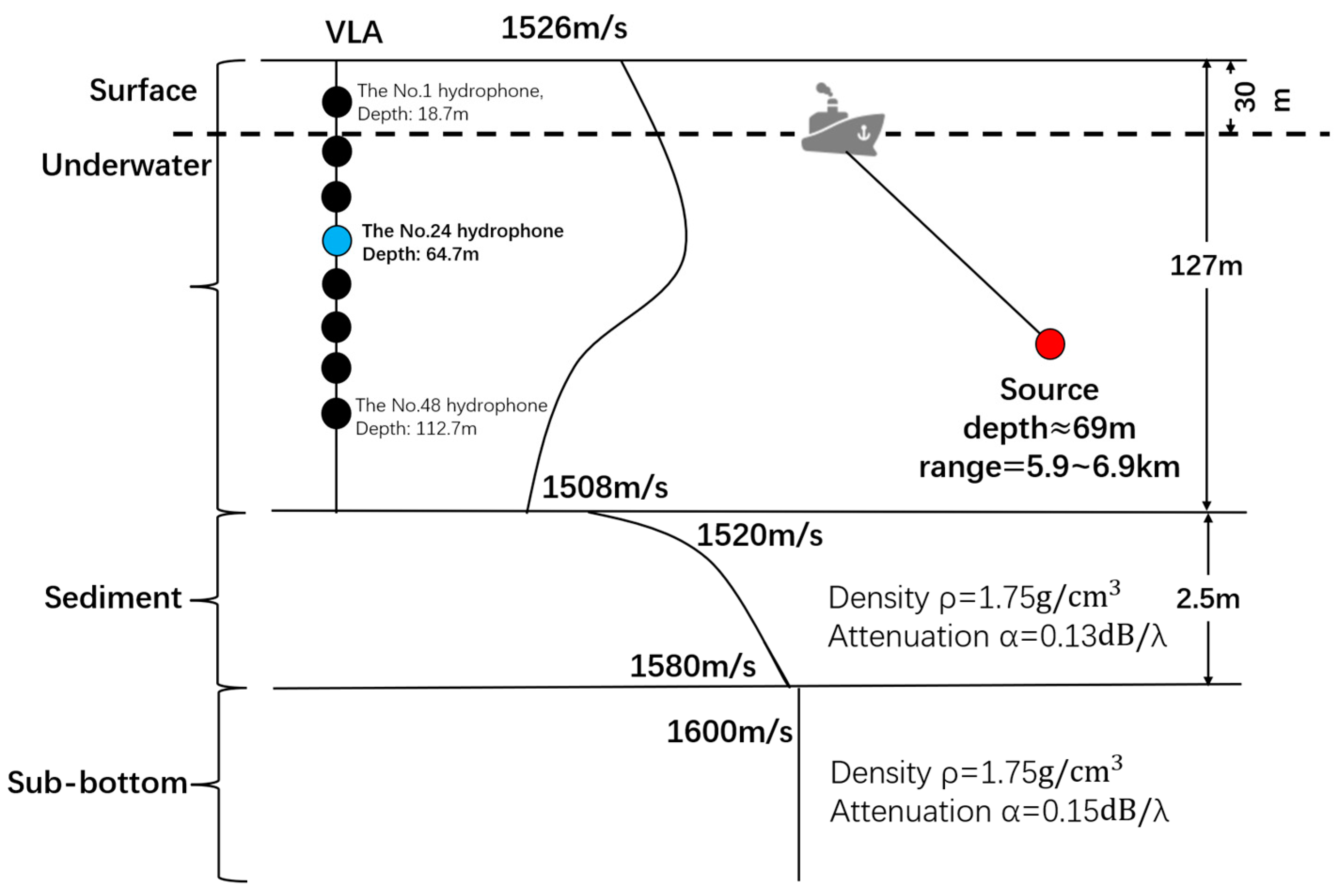
SACLANT Centre carried out an experiment in the shallow water area north of Elba Island on 26 and 27 October 1993 [25,26]. The 48-element VLA was used in the experiment, and the spacing was 2 m. The sound velocity profile and geometric structure throughout the experiment are shown in Figure 2. The experimental environment information of SACLANT 1993 is shown in Table 1. The depth of the top No.1 hydrophone was 18.7 m.
On 27 October, a mobile underwater source with a depth of approximately 69 m was deployed from a moving ship, as shown in Figure 2. The underwater source sends acoustic signals with a center frequency of about 170 Hz for 30 s and then stops for 30 s and repeats the cycle 10 times. The surface ship was driving. The frequency of its radiated noise was focused on the lower band from about 20 to 72 Hz. The initial distance from the VLA to the underwater sources was about 5.9 km, whereas the final distance was about 6.9 km with a speed of 3 knots (or 1.54 m/s) after about 10 min of travel. The transmitted signal of the underwater source was pseudorandom noise (PRN), and its frequency band was between 170 Hz and 220 Hz.
Generally speaking, the typical draft of shallow water vessels does not exceed 20 m. Therefore, this article uses 30 m as the recognition depth and divides all sound sources into two categories, i.e., water surface and underwater [27]. Sound source with a water depth of 0~30 m is surface sound source, and sound source with a water depth of 31 m or more is underwater sound source [1].
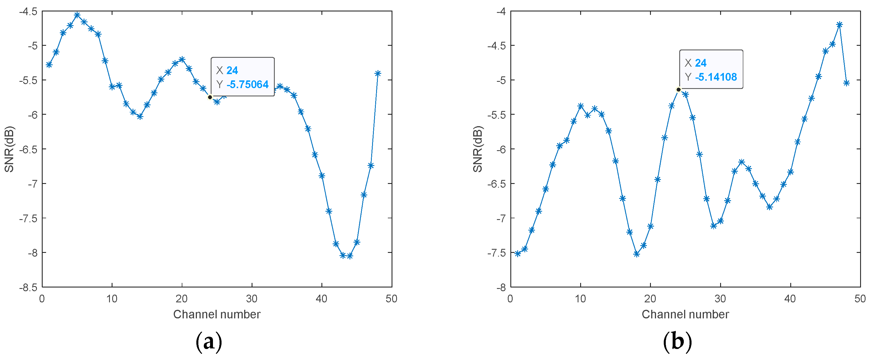
The SNR of the surface source is shown in Figure 3a. The SNR of the underwater source is shown in Figure 3b. To estimate the SNR of the surface source, the sound pressure levels in the 20–72 Hz band were compared with the levels outside this band, as shown in Figure 3a. Take Channel 24 for example, for which the SNR was −5.75. To estimate the SNR of the underwater source, the sound pressure levels in the 150–210 Hz band were compared with the levels outside this band, as shown in Figure 3b. For Channel 24 for example, the SNR was −5.14.
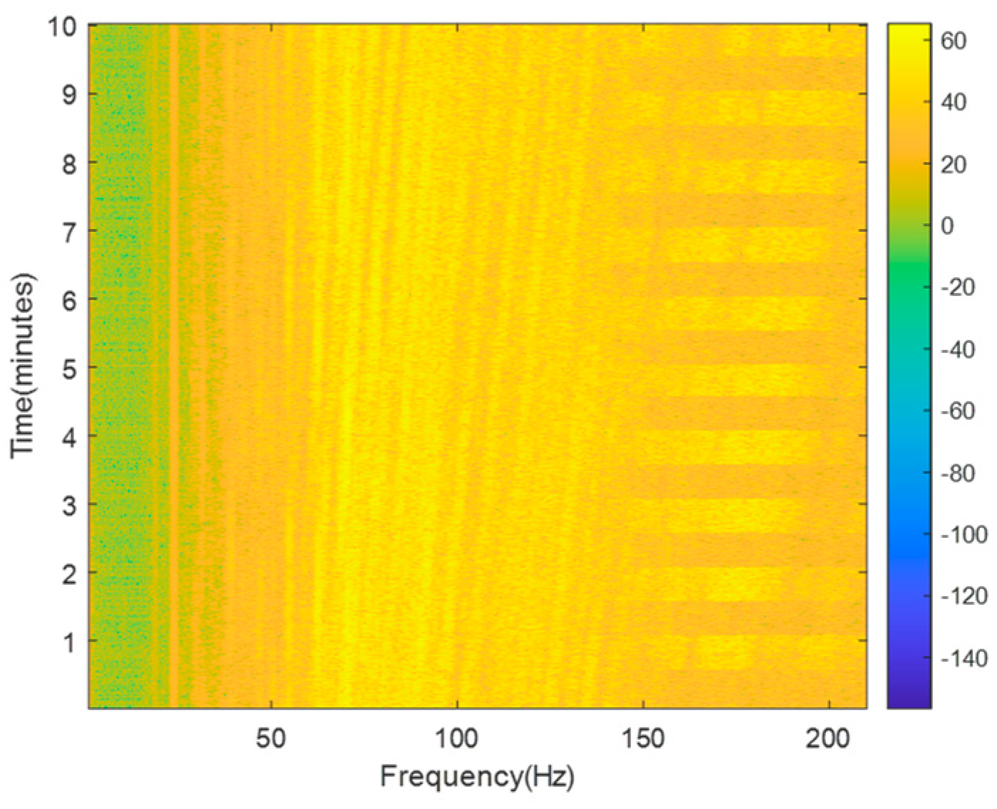
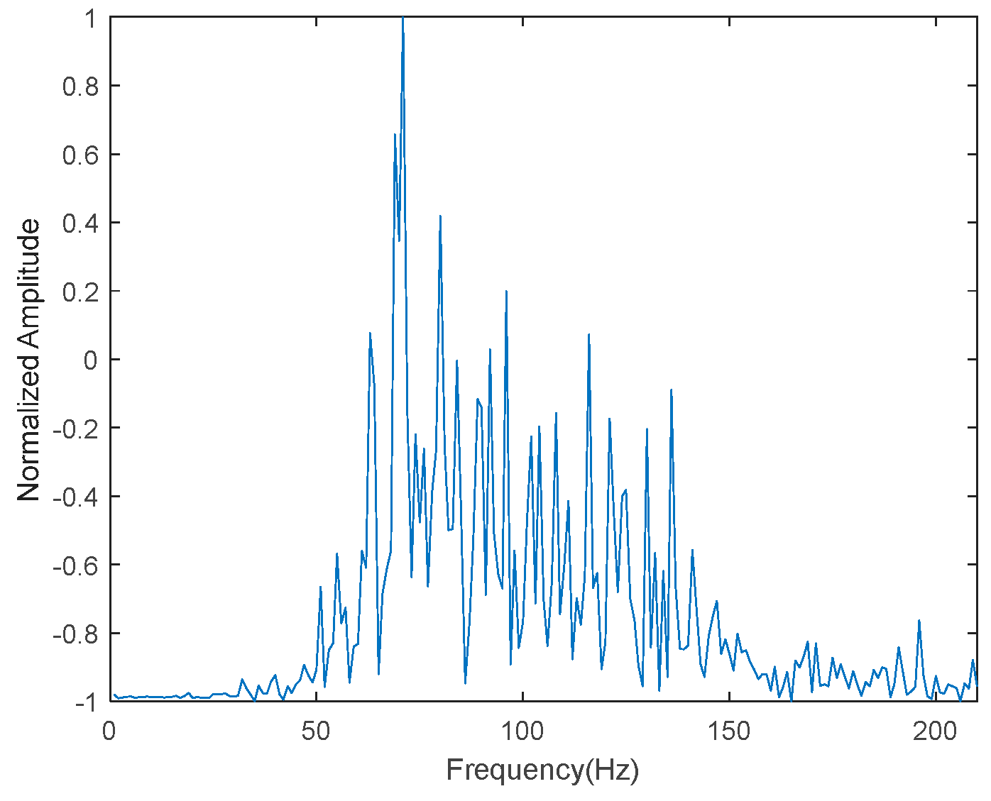
The recorded signal in the time and frequency domain are now displayed as follows. The spectrogram of the experimental data is shown in Figure 4, where the line spectra and discrete spectra are visible. The signal in the time domain is shown in Figure 5. It was found that the experimental samples were noisy but still fit the reality.

4.2. The Simulation Data

Firstly, hydrophone No. 24 was selected for analysis, and others are analyzed in Section 5.3. The sound energy distribution of 48 hydrophones on the VLA could have fluctuated due to multipath effects in shallow water, resulting in a different signal-to-noise ratio (SNR) on the receiver. Therefore, the SNR of the selected hydrophone needed to be a bit larger. The simulation data were generated by KRAKEN [26] using the real marine environment of SACLANT 1993.
In order to obtain sufficient training data, a distance interval of 0.1 km and a range of 4.0 to 7.0 km were set, resulting in a discrete number of 31. The depth interval was 1 m, the range was 1~90 m, and there were 90 discrete points. The sound signal had a wide frequency band and the frequency band width of the surface target was 20~72 Hz, with an interval of 0.5 Hz. Therefore, for each sample, the characteristic number of the surface target was 105. The frequency band width of the underwater target was 150~210 Hz, with an interval of 0.5 Hz. Therefore, for each sample, the characteristic number of the underwater target was 121. The simulation data were the spectrum and the unit was dB. The focal depth of 1 m~30 m corresponds to the surface signal source, whereas 30 m~90 m corresponds to the underwater signal source. Therefore, the number of all samples was 2790 (=31 × 90) and 930 (=31 × 30) surface target space samples and 1860 (=31 × 60) underwater target samples [1].
The 930 data samples from the surface signal source were labeled as tag 0. The 1860 underwater signal source data were labeled as tag 1. The corresponding water surface data and underwater data by channel were combined and the training set of each channel by row was formed to increase the generalization ability of the model. That is, the total size of the training set (pseudo data) for surface target detection was 2790 × 105, and the total size of the training set (pseudo data) for underwater target detection was 2790 × 121.
Finally, the simulation data were standardized to [−1, 1] by row to reduce the unfavorable effects caused by unique sample data.

4.3. The Experimental Data

In the experiment, the number of water surface data sampling points was 602,056 and the sampling rate was 1000 Hz. The length of time was 602.056 s, which is approximately 10 min. A total of 2000 points were taken as samples and the experimental data were segmented, with 1800 overlapping points. For the surface target, the surface sample experimental data were a 3001 × 2000 matrix. Fourier transform was performed on the matrix by row. Only frequency points within the [20, 72] Hz range were retained. The ultimate sample was a 3001 × 105 matrix. All data were normalized line by line to [−1, 1], all samples were marked as 0, and a test set was obtained for water surface target detection.
In the experiment, there were 297,244 underwater data sampling points, with a sampling rate of 1000 Hz and a duration of 297.244 s—about 5 min. Among them, 2000 points were taken as samples, and the experimental data were segmented. There were 1800 overlapping points, resulting in a matrix of 1477 × 2000. A total of 2000 points were taken as samples, and the sea trial data were processed in sections. Fourier transform was performed on the matrix by row, and frequency points were only reserved within the [150, 210] Hz range.
The ultimate sample was a 1477 × 121 matrix. All data were normalized by row to [−1, 1], all samples were marked as 1, and the test set of underwater target detection was obtained.

4.4. Feature Extraction

Because all the sampled data were complex and could not be directly used in the machine learning algorithms, it needed to be processed first. There are two kinds of feature extraction methods. The first one is to take the modules of all complex points and use the amplitude information to build the model. The second one is to separate the real part and the imaginary part as the two kinds of features of a point and provide the amplitude information and phase information at the same time.
(1)
Using Modules as Features
For the data set collected by each channel, the data were normalized by row before training so that the pre-processed data were limited to the range of [−1, 1] and the interference of special sample data was eliminated. For the experimental data set, all data were normalized by row to [−1, 1], all samples of water targets were marked as 0, and all samples of underwater targets were marked as 1. For a realistic dataset, after normalizing to [−1, 1] by row, 930 data samples from the water surface signal source were labeled as 0 and 1860 underwater signal source data were labeled as 1. The corresponding water surface data and underwater data were combined by channel and a training set was formed for each channel by row scrambling, increasing the generalization ability of the model. That is, the total size of the test set (experimental data) for surface target detection was 3001 × 105, the total size of the test set (experimental data) for underwater target detection was 1477 × 121, the total size of the training set (simulation data) for surface target detection was 2790 × 105, and the total size of the training set (simulation data) for underwater target detection was 2790 ×121.
(2)
Using Real and Imaginary Parts as Features
For the data set collected by each channel, the real part and imaginary part of all complex numbers were first disassembled, and then the real part and imaginary part of the same sample were combined into a row. At this time, the data of the surface target changed from 105 features to 210 features, and the data of the underwater target changed from 121 features to 242 features. Next, the same normalization, marking of data sets, merging of samples of realistic data sets, and scrambling of samples were carried out as above. The total size of the test set (experimental data) for surface target detection was 3001 × 210 (210 = 105 × 2), and the total size of the test set (experimental data) for underwater target detection was 1477 × 242(242 = 121 × 2), the total size of the training set (simulation data) for surface target detection was 2790 × 210, and the total size of the training set (simulation data) for underwater target detection was 2790 × 242.

5. Results and Analyses

5.1. Results of GBDT

5.1.1. Evaluation of Surface Target Detection Model

In this section, the GBDT model was used to analyze VLA with a bandwidth of [20, 72] Hz. The simulated data received by a single hydrophone were generated using KRAKEN, as detailed in Section 4.2. The experimental data were SACRANT 1993, as detailed in Section 4.3.
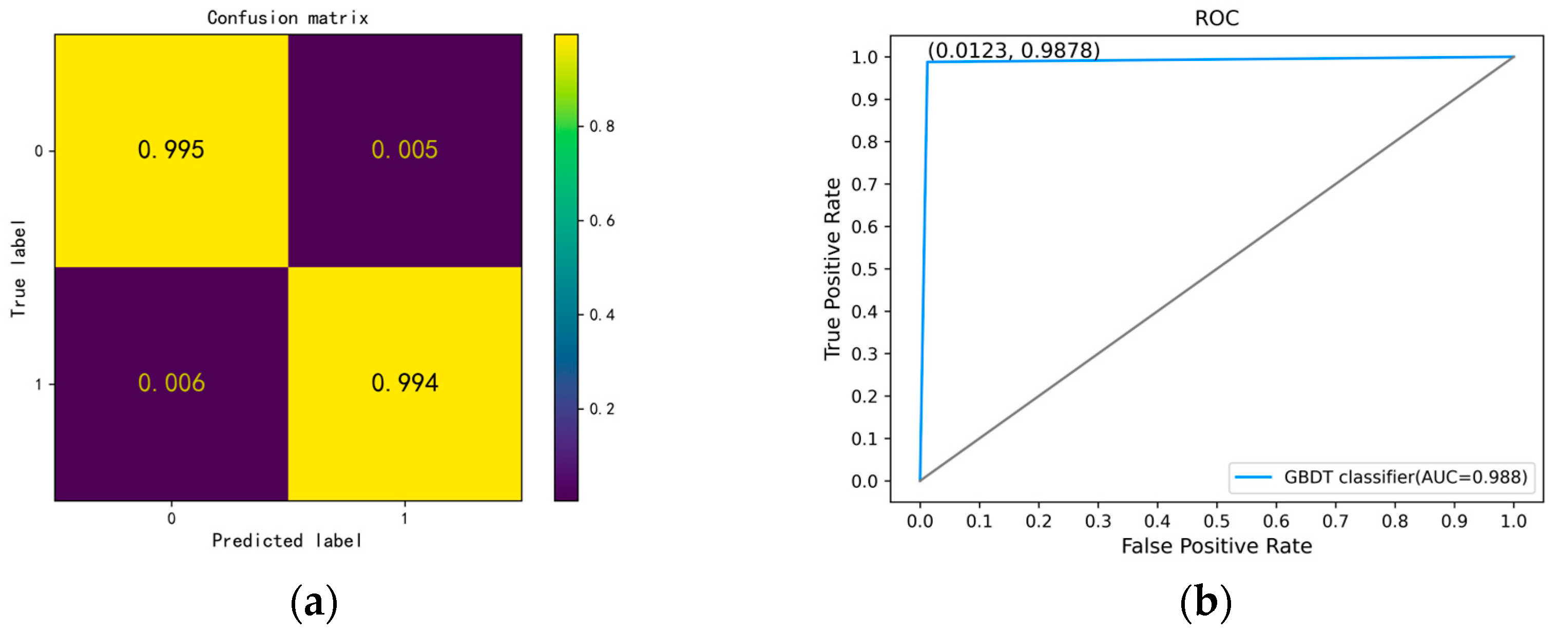
(1) For surface models using modules as features, the hyperparameters of the No. 24-GBDT-mod-surface (classification of water surface targets using module features based on the GBDT algorithm, named similarly hereafter) model are as follows: a step size of 0.1, a maximum number of iterations of 120, a maximum depth of 10 for the tree, a minimum number of samples for leaf nodes of 13, a score of 19 for internal node subdivisions, and a maximum number of features divided by 2. The precision, recall, F1, and accuracy of the simulation data were 0.9942, 0.9885, 0.9913, and 0.9946, respectively, as shown in Table 2. From Table 2, it can be seen that the trained model achieved good results in accuracy and recall, and the experimental accuracy was also very high. The confusion matrix diagram is shown in Figure 6a. The receiver operating characteristic (ROC) diagram is shown in Figure 6b, where labels 0 and 1 represent S/U sources, respectively. Among them, 99.5% of surface sources were correctly classified as surface sources, and 0.5% of surface sources were misclassified as underwater sources. A total of 99.4% of underwater sources were correctly classified as underwater sources, and 0.6% of underwater sources were misclassified as surface sources.
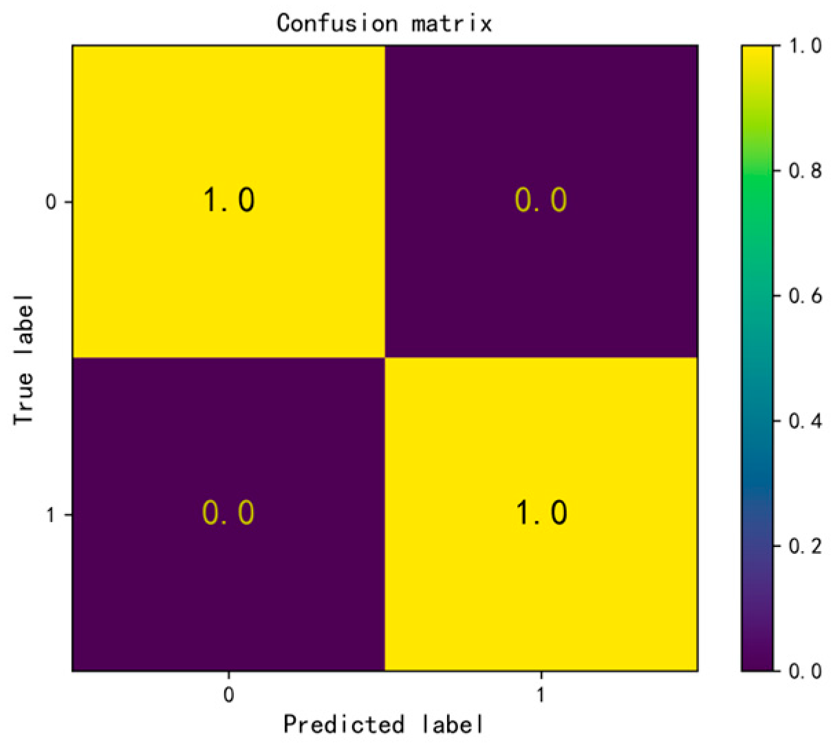
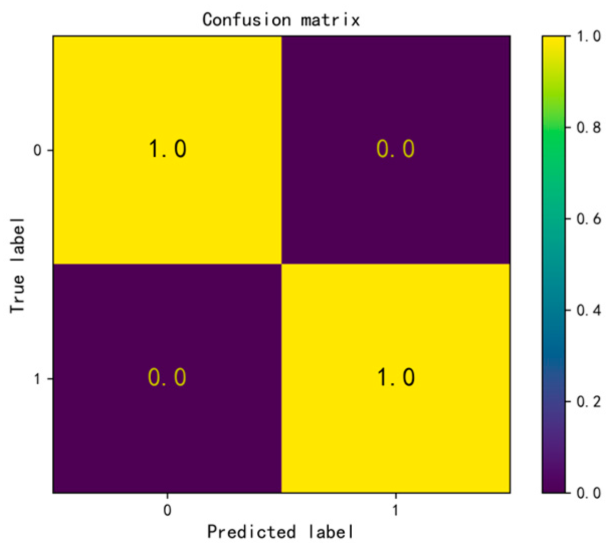
Then, the No. 24 hydrophone was used to analyze the test data and its confusion matrix diagram was obtained, as shown in Figure 7. Among them, 100% of surface sources were correctly classified as surface sources, and 0% of surface sources were misclassified as underwater sources. Because the test data set was all 0 or all 1, only accuracy could be deducted in the confusion matrix diagram. For the No. 24 hydrophone, the test accuracy was 1.0.
The above section only analyzed the data from the No. 24 hydrophone. In the next section, GBDT is used to analyze data from all hydrophones with water source bandwidth. A threshold of 0.9 was manually set to determine whether the training was successful.
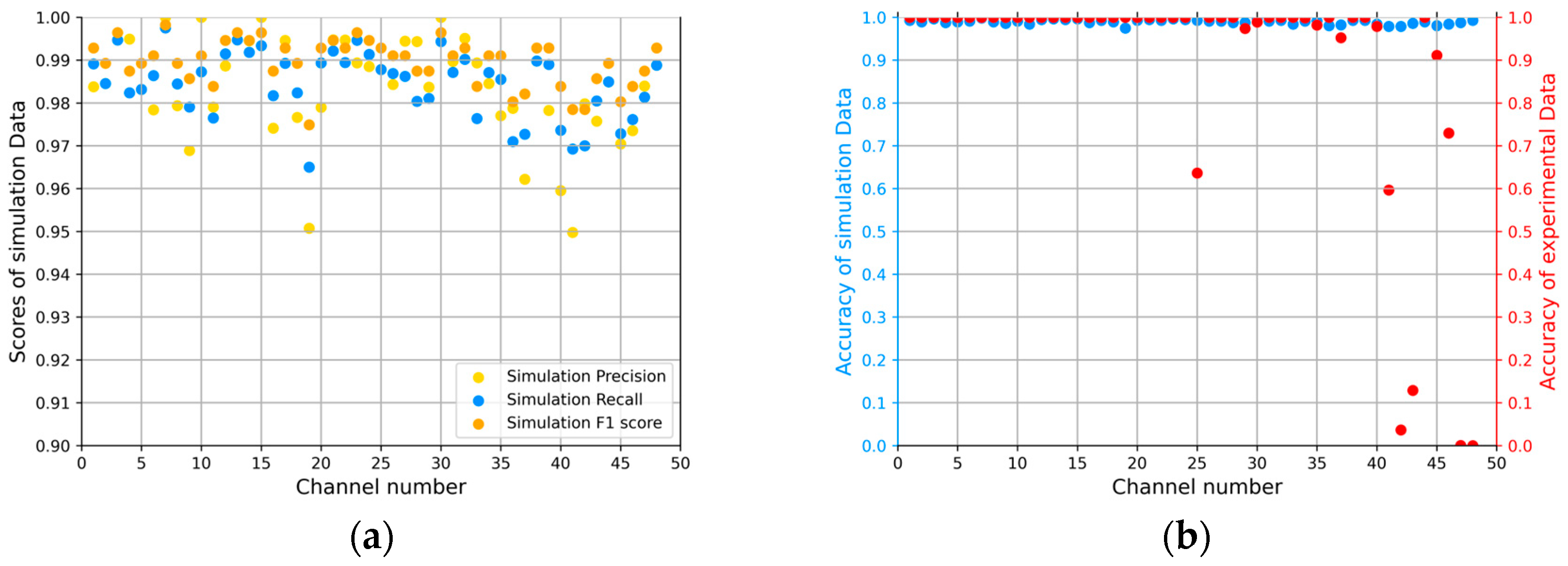
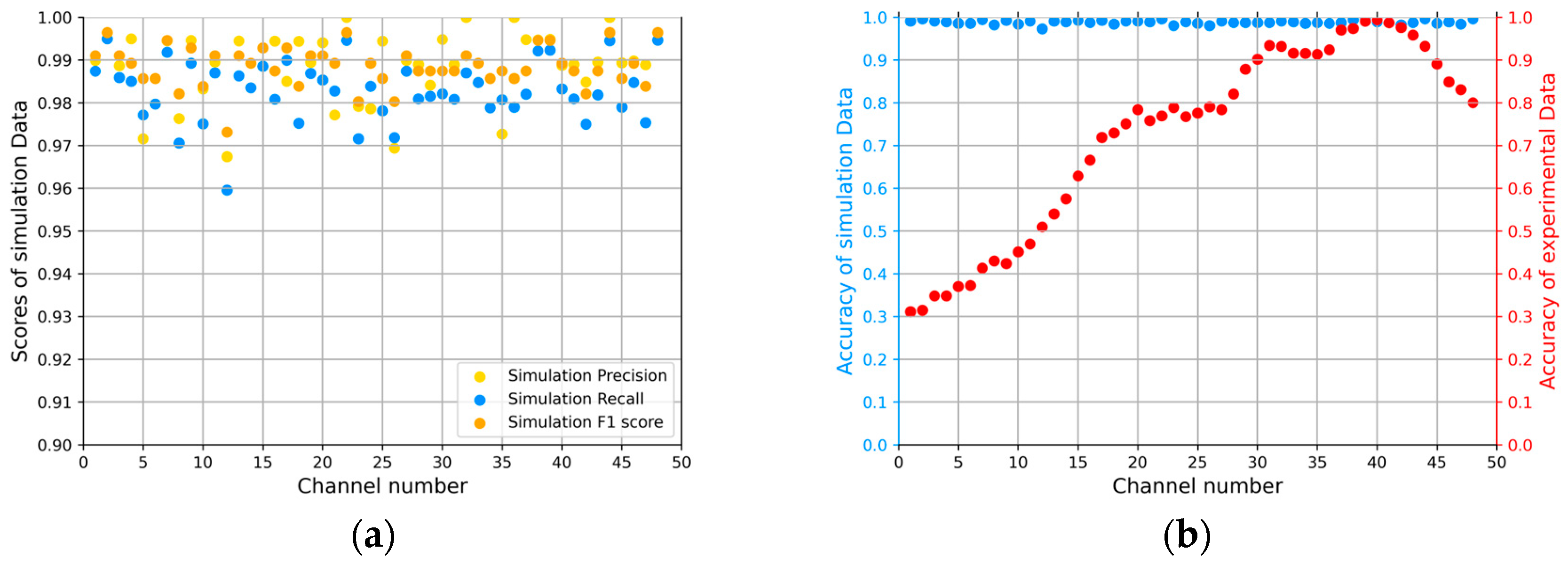
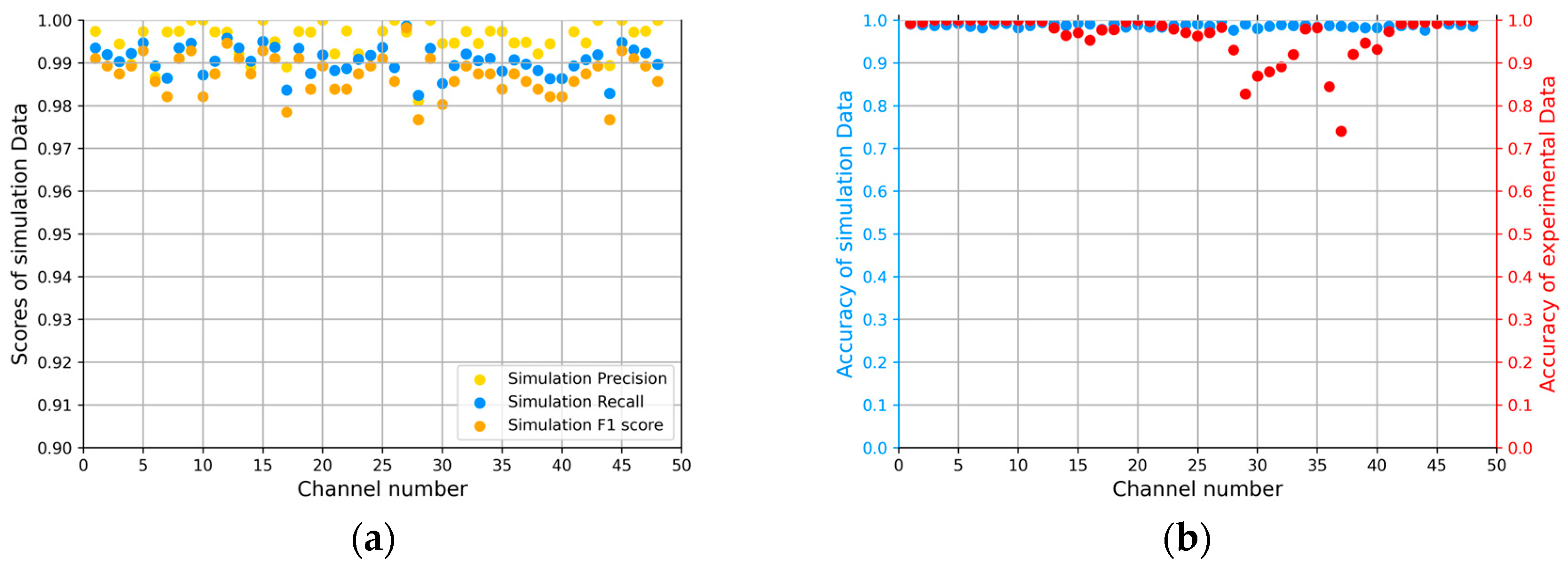
For a surface model using modules as features, the training data for each hydrophone were a 2790 × 105 array, and the test data were a 3001 × 105 array. See Section 4.2 and Section 4.3 for details. The verification results (precision, recall, and F1) of the simulation data for water surface targets characterized by modules are shown in Figure 8a. The comparison diagram of the verification accuracy and test accuracy is shown in Figure 8b.
As can be seen from Figure 8, out of 48 hydrophones, the threshold of the simulation data reached 0.9, but only 41 hydrophones (numbered 1, 2, 3, 4, 5, 6, 7, 8, 9, 10, 11, 12, 13, 14, 15, 16, 17, 18, 19, 20, 21, 22, 23, 24, 26, 27, 28, 29, 30, 31, 32, 33, 34, 35, 36, 37, 38, 39, 40, 44, 45) successfully reached the threshold of 0.9 when using the experimental data.
(2) For surface models using real and imaginary values as features, the hyperparameters of the No. 24-GBDT-com-surface model were as follows: a step size of 0.1, a maximum number of iterations of 160, a maximum depth of 7 for the tree, a minimum number of samples for leaf nodes of 15, a score of 17 for internal node subdivisions, and a maximum number of features divided by 16. The precision, recall, F1, and accuracy of the simulation data were 0.9892, 0.9786, 0.9839, and 0.9892, respectively, as shown in Table 2. The confusion matrix diagram is shown in Figure 9a, and the ROC diagram is shown in Figure 9b. Here, 98.9% of surface sources were correctly classified, and 1.1% were incorrectly classified as underwater sources; 98.9% of underwater sources were correctly classified, and 1.1% were incorrectly classified as surface sources.
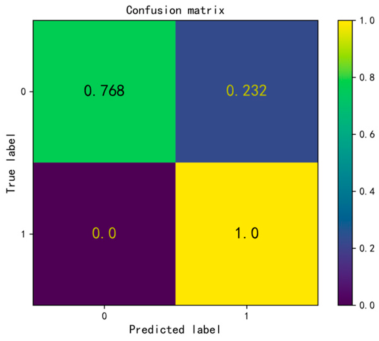
Then, the No. 24 hydrophone was used to analyze the test data and its confusion matrix diagram was obtained, as shown in Figure 10. Among them, 76.8% of surface sources were correctly classified as surface sources, and 23.2% of surface sources were misclassified as underwater sources. The test accuracy of the No. 24 hydrophone was 0.768.
The above section only analyzed the data from the No. 24 hydrophone. In the next section, GBDT is used to analyze data from all hydrophones with water source bandwidth. A threshold of 0.9 was manually set to determine whether the training was successful.
For a surface model using real and imaginary values as features, the training data for each hydrophone were a 2790 × 210 array, and the test data were a 3001 × 210 array. See Section 4.4 for details. The verification results of the simulation data of water surface targets characterized by real and imaginary values are shown in Figure 11a. The comparison diagram of the verification accuracy and test accuracy is shown in Figure 11b.
As can be seen from Figure 11, out of 48 hydrophones, the threshold of the simulation data reached 0.9, but only 15 hydrophones (numbered 30, 31, 32, 33, 34, 35, 36, 37, 38, 39, 40, 41, 42, 43, 44) successfully reached the threshold of 0.9 when using the experimental data.

5.1.2. Evaluation of Underwater Target Detection Model

In this section, the GBDT model is used to analyze the VLA with a bandwidth of [150, 210] Hz. The simulated data received by a single hydrophone were generated using KRAKEN. See Section 4.2 for details. This section selects the No. 24 hydrophone for simulation data and corresponding network training. The test experimental data were a 1477 × 121 array; see Section 4.3 for details.
(1) For underwater models using modules as features, the hyperparameters of the No. 24-GBDT-mod-underwater model were as follows: The step size was 0.1, the maximum number of iterations was 160, the maximum depth of the tree was 15, the minimum number of samples for leaf nodes was 8, the internal node subdivision score was 7, and the maximum number of features divided was 4. The precision, recall, F1, and accuracy of the simulation data were 0.9769, 1, 0.9883, and 0.9839, respectively, as shown in Table 3. The confusion matrix diagram is shown in Figure 12a, and the ROC diagram is shown in Figure 12b. Here, 99.1% of surface sources were correctly classified, and 0.9% were incorrectly classified as underwater sources; 97.7% of underwater sources were correctly classified, and 2.3% were incorrectly classified as surface sources.
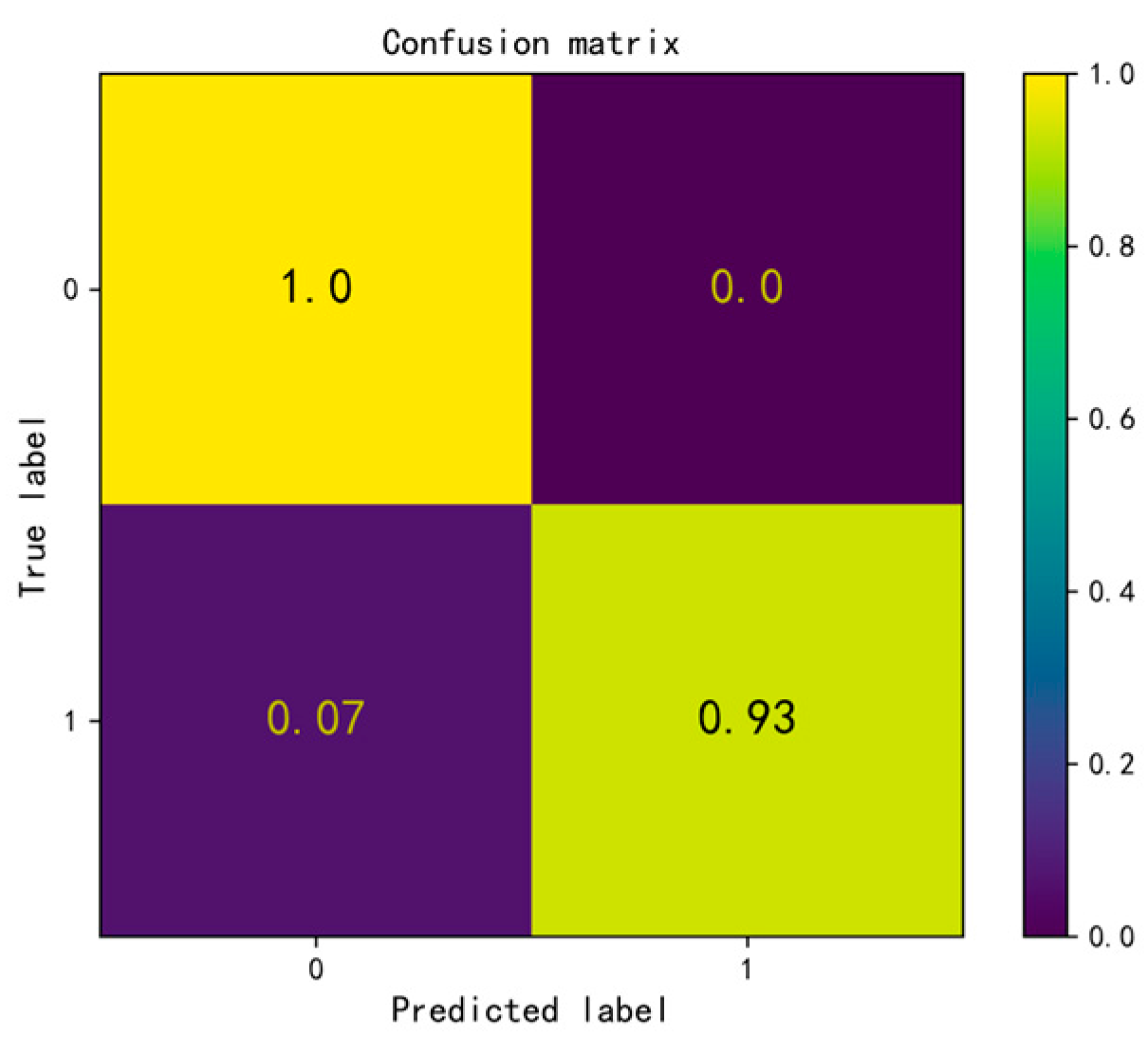
Then, the No. 24 hydrophone was used to analyze the test data and its confusion matrix diagram was obtained, as shown in Figure 13. Among them, 93% of underwater sources were correctly classified as underwater sources, and 7% of underwater sources were misclassified as surface sources. The test accuracy of the No. 24 hydrophone was 0.93.
The above section only analyzed the data from the No. 24 hydrophone. In the next section, GBDT is used to analyze data from all hydrophones with underwater source bandwidth. A threshold of 0.9 was manually set to determine whether the training was successful.
For underwater models using modules as features, the training data for each hydrophone were a 2790 × 121 array, and the test data were a 1477 × 121 array. See Section 4.2 and Section 4.3 for details. The verification results of underwater target simulation data characterized by modules are shown in Figure 14a. The comparison diagram of the verification accuracy and test accuracy is shown in Figure 14b.
As can be seen from Figure 14, out of 48 hydrophones, the threshold of the simulation data reached 0.9, but only 35 hydrophones (numbered 1, 2, 3, 4, 5, 6, 7, 8, 9, 10, 11, 12, 13, 19, 20, 21, 22, 23, 24, 25, 26, 27, 32, 33, 34, 35, 39, 40, 41, 42, 43, 45, 46, 47, 48) successfully reached the threshold of 0.9 when using experimental data.
(2) For underwater models using real and imaginary values as features, the hyperparameters of the No. 24-GBDT-com-underwater model were as follows: The step size was 0.1, the maximum number of iterations was 130, the maximum depth of the tree was 16, the minimum number of samples for leaf nodes was 4, the internal node subdivision score was 2, and the maximum number of features divided was 3. The precision, recall, F1, and accuracy of the simulation data were 0.9918, 0.9916, 0.9918, and 0.9892, respectively, as shown in Table 3. The confusion matrix diagram is shown in Figure 15a, and the ROC diagram is shown in Figure 15b. Here, 98.7% of surface sources were correctly classified, and 1.3% were incorrectly classified; 99.2% of underwater sources were correctly classified, and 0.8% were incorrectly classified.
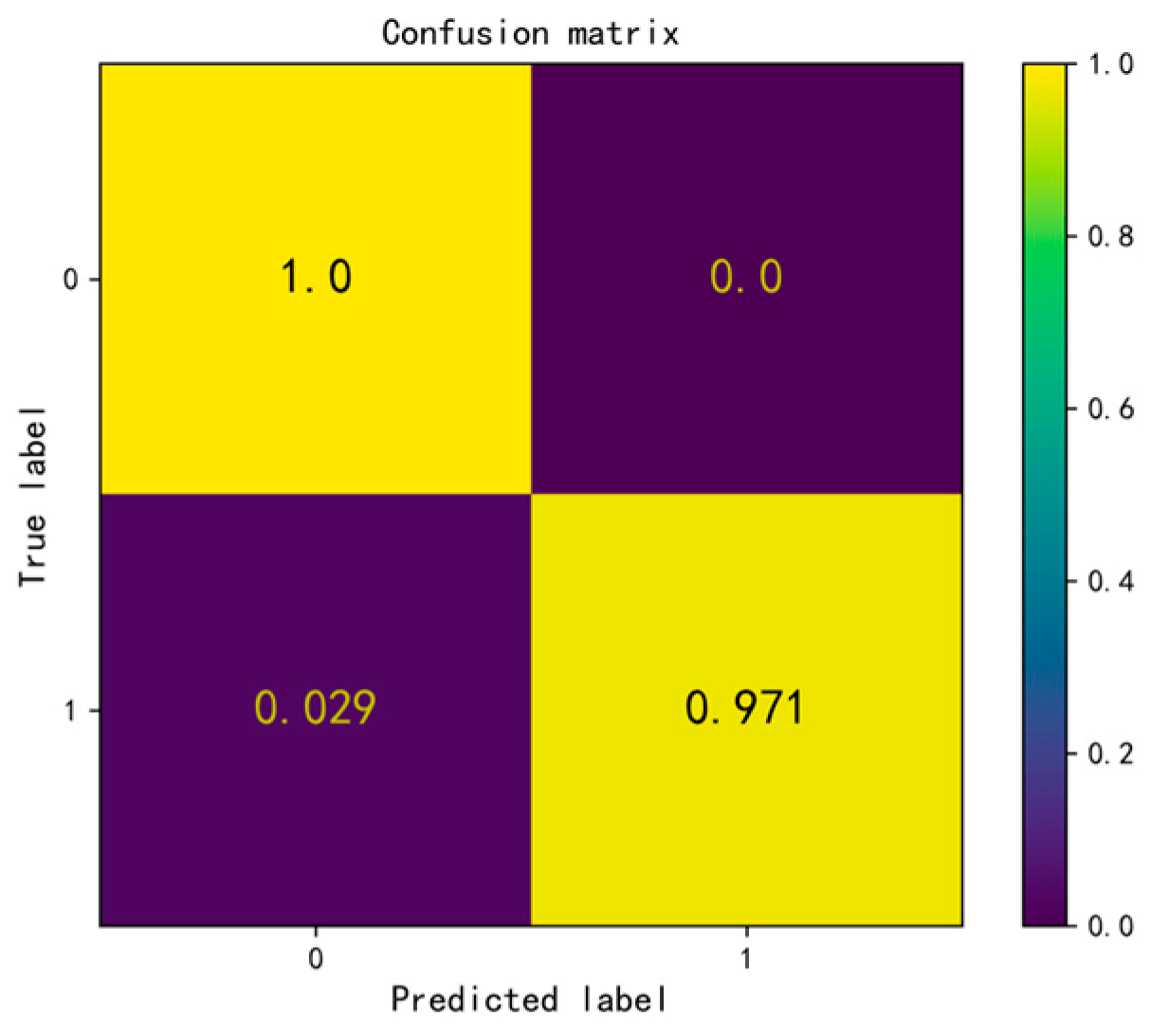
Then, the No. 24 hydrophone was used to analyze the test data and its confusion matrix diagram was obtained, as shown in Figure 16. Among them, 97.1% of underwater sources were correctly classified as underwater sources, and 2.9% of underwater sources were misclassified as surface sources. The test accuracy of the No. 24 hydrophone was 0.971.
The above section only analyzed the data from the No. 24 hydrophone. In the next section, GBDT is used to analyze data from all hydrophones with underwater source bandwidth. A threshold of 0.9 was manually set to determine whether the training was successful.
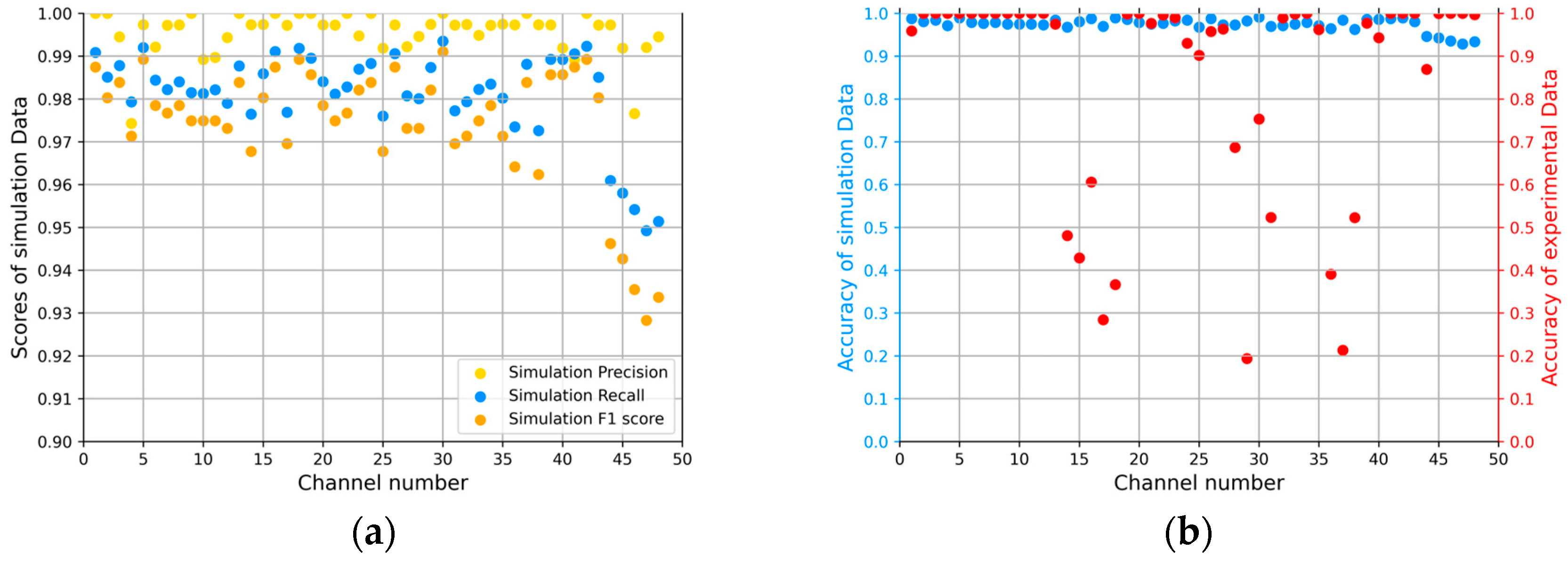
For underwater models using real and imaginary values as features, the training data for each hydrophone were a 2790 × 242 array, and the test data were a 1477 × 242 array. See Section 4.4 for details. The verification results of the simulation data of water surface targets characterized by real and imaginary values are shown in Figure 17a. The comparison diagram of the verification accuracy and test accuracy is shown in Figure 17b.
As can be seen from Figure 17, out of 48 hydrophones, the threshold of the simulation data reached 0.9, but only 42 hydrophones (numbered 1, 2, 3, 4, 5, 6, 7, 8, 9, 10, 11, 12, 13, 14, 15, 16, 17, 18, 19, 20, 21, 22, 23, 24, 25, 26, 27, 28, 33, 34, 35, 38, 39, 40, 41, 42, 43, 44, 45, 46, 47, 48) successfully reached the threshold of 0.9 when using the experimental data.

5.2. Results of LightGBM

In this section, the LightGBM model is used to analyze the VLA. The simulation data received by a single hydrophone were generated using KRAKEN. See Section 4.2 for details. This section selects the No. 24 hydrophone for simulation data and corresponding network training.

5.2.1. Evaluation of Water Surface Target Detection Model

(1) For surface models using modules as features, the hyperparameters of the No. 24-LightGBM-mod-surface model were as follows: a step size of 0.09, a number of leaves on a tree of 20, and a maximum depth of 7. Without resampling, 90% of the data were randomly selected, and 30% of the features were randomly selected in each iteration. The precision, recall, F1, and accuracy of the simulation data were 0.9868, 0.9973, 0.9921, and 0.9892, respectively, as shown in Table 4. The confusion matrix diagram is shown in Figure 18a, and the ROC diagram is shown in Figure 18b. Here, 99.2% of surface sources were correctly classified, and 0.8% were incorrectly classified; 98.7% of underwater sources were correctly classified, and 1.3% were incorrectly classified.
Then, the No. 24 hydrophone was used to analyze the test data and its confusion matrix diagram was obtained, as shown in Figure 19. Here, 100% of surface sources were correctly classified, and 0% were incorrectly classified. The test accuracy of the No. 24 hydrophone was 1.
The above section only analyzed the data from the No. 24 hydrophone. In the next section, LightGBM is used to analyze data from all hydrophones with water source bandwidth. A threshold of 0.9 was manually set to determine whether the training was successful.
For a surface model using modules as features, the training data for each hydrophone were a 2790 × 105 array, and the test data were a 3001 × 105 array. See Section 4.2 and Section 4.3 for details. The verification results of the simulation data for water surface targets characterized by modules are shown in Figure 20a. The comparison diagram of the verification accuracy and test accuracy is shown in Figure 20b.
As can be seen from Figure 20, out of 48 hydrophones, the threshold of the simulation data reached 0.9, but only 40 hydrophones (numbered 1, 2, 3, 4, 5, 6, 7, 8, 9, 10, 11, 12, 13, 14, 15, 16, 17, 18, 19, 20, 21, 22, 23, 24, 25, 26, 27, 28, 29, 30, 32, 33, 34, 35, 36, 37, 38, 39, 44, 45) successfully reached the threshold of 0.9 when using the experimental data.
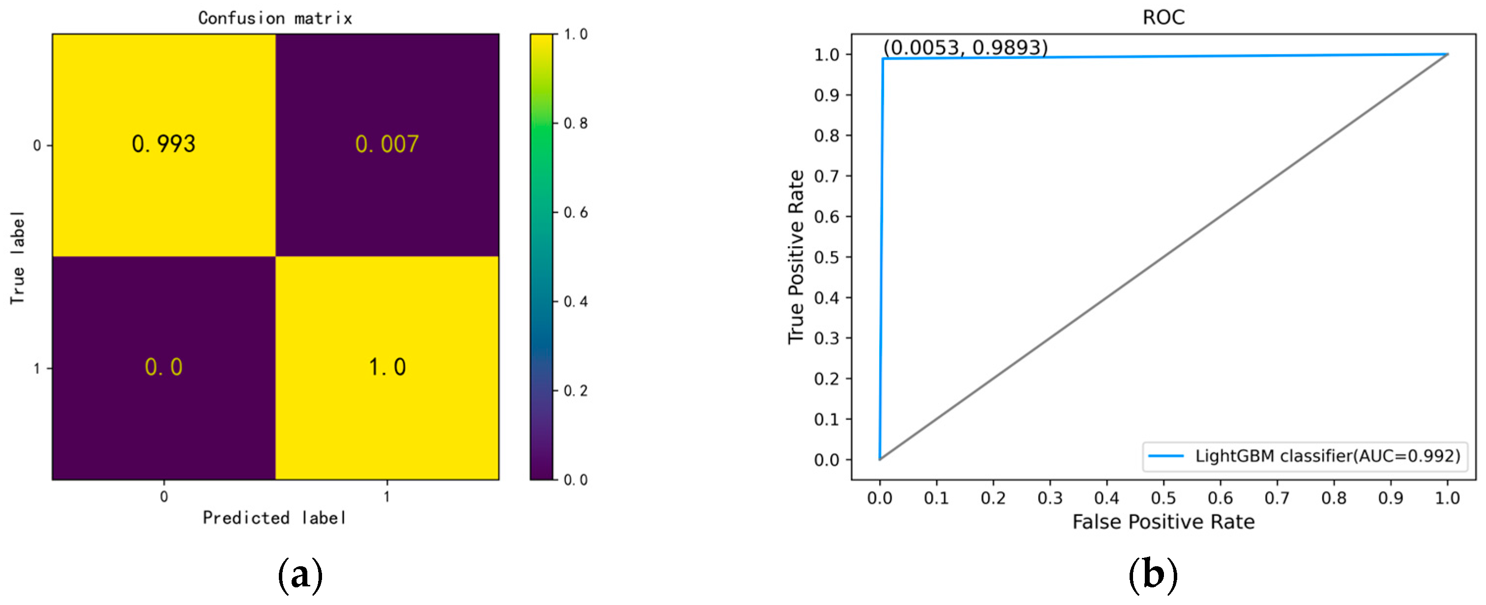
(2) For surface models using real and imaginary values as features, the hyperparameters of the No. 24-LightGBM-com-surface model were as follows: The step size was 0.084, the number of leaves on a tree was 340, and the maximum depth of the tree was 4. Without resampling, 60% of the data were randomly selected, and 20% of the features were randomly selected in each iteration. The precision, recall, F1, and accuracy of the simulation data were 1, 0.9947, 0.9974, and 0.9964, respectively, as shown in Table 4. The confusion matrix diagram is shown in Figure 21a, and the ROC diagram is shown in Figure 21b. Here, 99.3% of surface sources were correctly classified, and 0.7% of samples were incorrectly classified; 100% of underwater sources were correctly classified, and 0% were incorrectly classified.
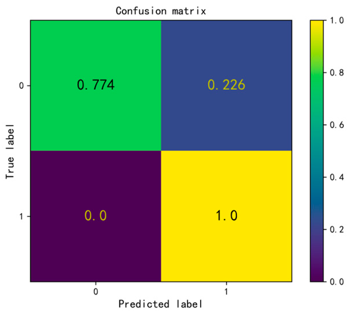
Then, the No. 24 hydrophone was used to analyze the test data and its confusion matrix diagram was obtained, as shown in Figure 22. Here, 77.4% of surface sources were correctly classified, and 22.6% of samples were incorrectly classified. The test accuracy of the No. 24 hydrophone was 0.774.
The above section only analyzed the data from the No. 24 hydrophone. In the next section, LightGBM is used to analyze data from all hydrophones with water source bandwidth. A threshold of 0.9 was manually set to determine whether the training was successful.
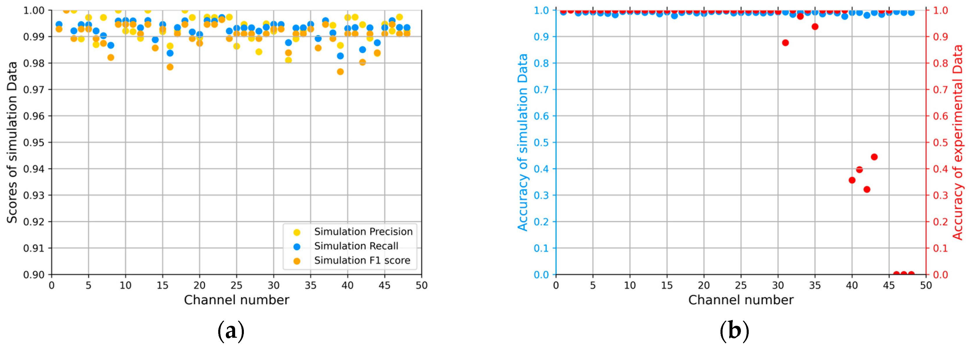
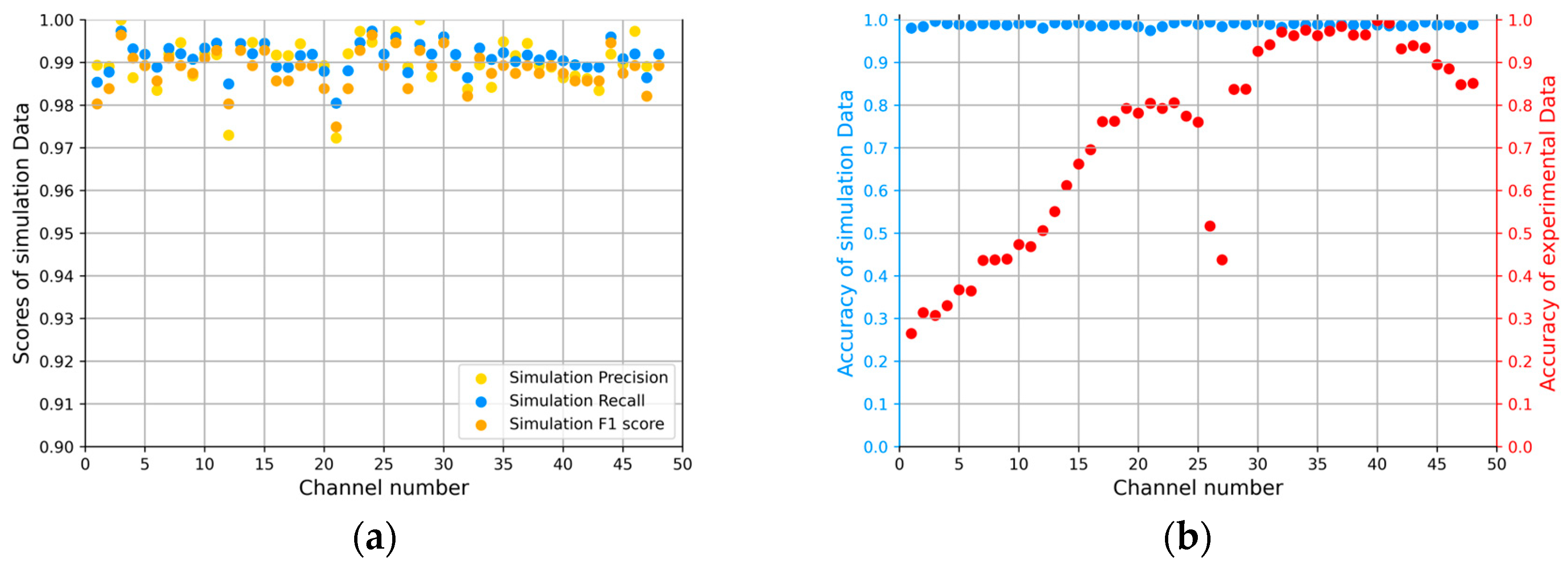
For surface models using real and imaginary values as features, the training data for each hydrophone were a 2790 × 210 array, and the test data were a 3001 × 210 array. See Section 4.4 for details. The verification results of the simulation data of water surface targets characterized by real and imaginary values are shown in Figure 23a. The comparison diagram of the verification accuracy and test accuracy is shown in Figure 23b.
As can be seen from Figure 23, out of 48 hydrophones, the threshold of the simulation data reached 0.9, but only 15 hydrophones (numbered 30, 31, 32, 33, 34, 35, 36, 37, 38, 39, 40, 41, 42, 43, 44) successfully reached the threshold of 0.9 when using experimental data.

5.2.2. Evaluation of Underwater Target Detection Model

In this section, the LightGBM model is used to analyze the VLA with a bandwidth of [150, 210] Hz. The simulated data received by a single hydrophone were generated using KRAKEN. See Section 4.2 for details. This section selects the No. 24 hydrophone for simulation data and the corresponding network training. The test experimental data were a 1477 × 121 array; see Section 4.3 for details.
(1) For underwater models using modules as features, the hyperparameters of the No. 24-LightGBM-mod-underwater model were as follows: The step size was 0.094, the number of leaves on a tree was 100, and the maximum depth of the tree was 8. Without resampling, 80% of the data were randomly selected, and 60% of the features were randomly selected in each iteration. The precision, recall, F1, and accuracy of the simulation data were 0.9489, 0.9920, 0.9699, and 0.9588, respectively, as shown in Table 5. The confusion matrix diagram is shown in Figure 24a, and the ROC diagram is shown in Figure 24b. Here, 97% of surface sources were correctly classified, and 3% were incorrectly classified; 94.8% of underwater sources were correctly classified, and 5.2% were incorrectly classified.
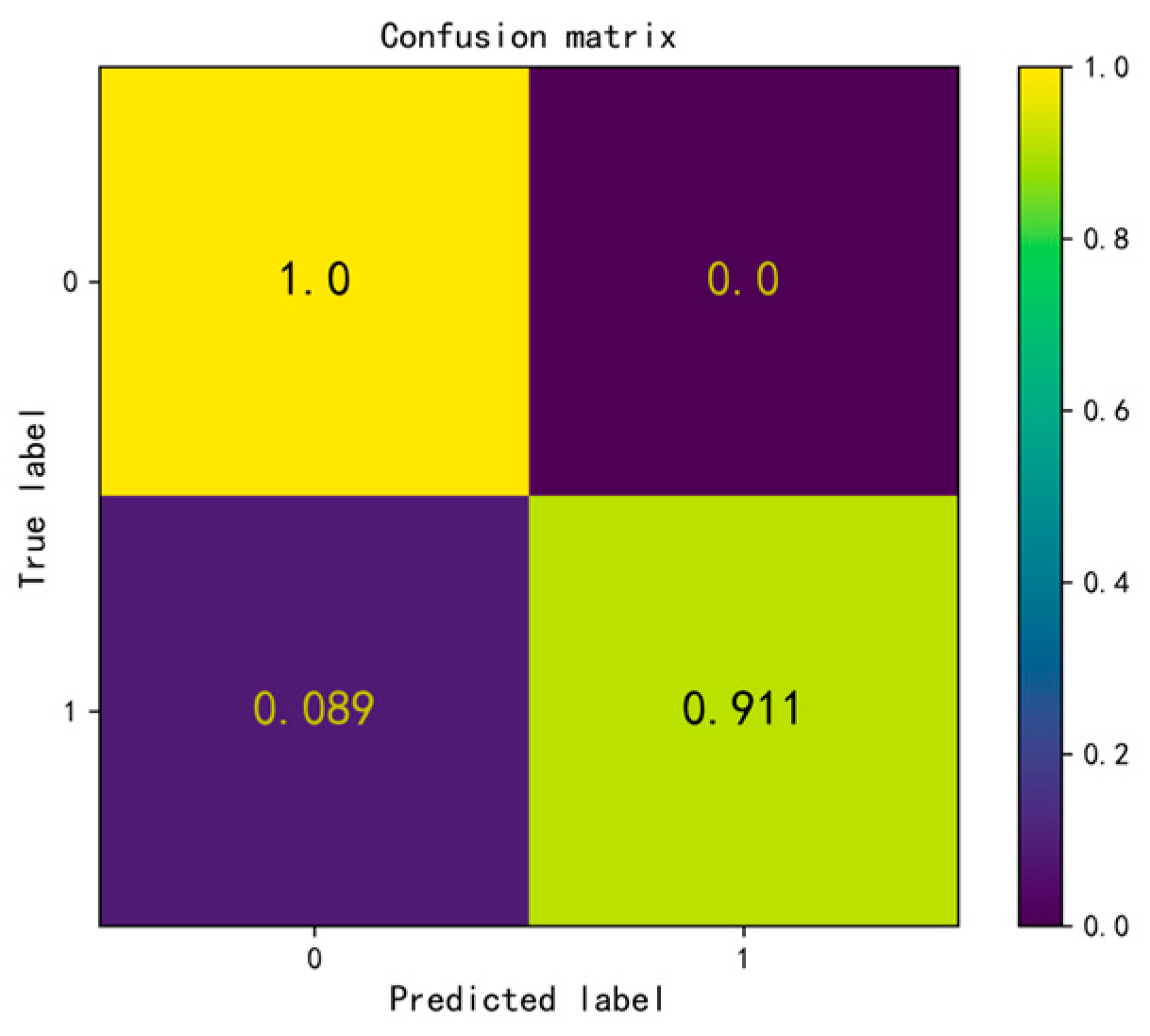
Then, the No. 24 hydrophone was used to analyze the test data and its confusion matrix diagram was obtained, as shown in Figure 25. Here, 91.1% of underwater sources were correctly classified, and 8.9% were incorrectly classified. The test accuracy of the No. 24 hydrophone was 0.911.
The above section only analyzed the data from the No. 24 hydrophone. In the next section, LightGBM is used to analyze data from all hydrophones with underwater source bandwidth. A threshold of 0.9 was manually set to determine whether the training was successful.
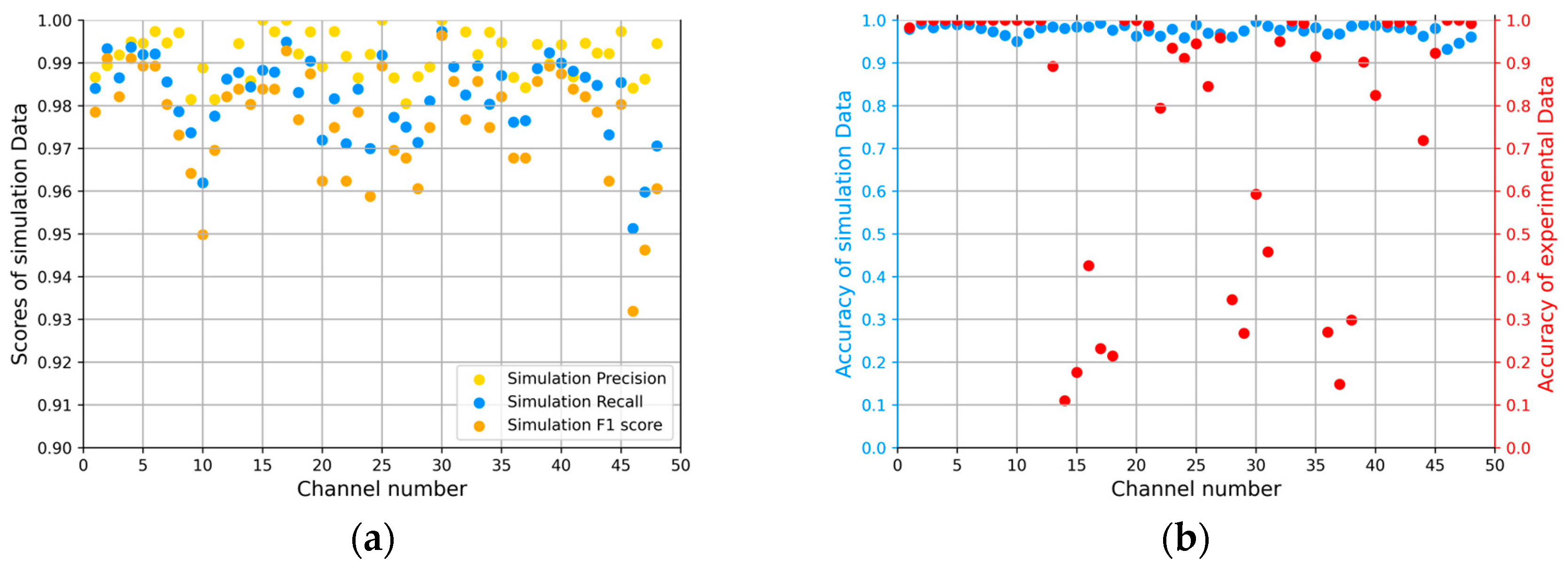
For underwater models using modules as features, the training data for each hydrophone were a 2790 × 121 array, and the test data were a 1477 × 121 array. See Section 4.2 and Section 4.3 for details. The verification results of the underwater target simulation data characterized by modules are shown in Figure 26a. The comparison diagram of the verification accuracy and test accuracy is shown in Figure 26b.
As can be seen from Figure 26, out of 48 hydrophones, the threshold of the simulation data reached 0.9, but only 31 hydrophones (numbered 1, 2, 3, 4, 5, 6, 7, 8, 9, 10, 11, 12, 19, 20, 21, 23, 24, 25, 27, 32, 33, 34, 35, 39, 41, 42, 43, 45, 46, 47, 48) successfully reached the threshold of 0.9 when using the experimental data.
(2) For underwater models using real and imaginary values as features, the hyperparameters of the No. 24-LightGBM-com-underwater model were as follows: The step size was 0.1, the number of leaves on a tree was 52, and the maximum depth of the tree was 6. Without resampling, 70% of the data were randomly selected, and 90% of the features were randomly selected in each iteration. The precision, recall, F1, and accuracy of the simulation data were 0.9947, 0.9920, 0.9933, and 0.9910, respectively, as shown in Table 5. The confusion matrix diagram is shown in Figure 27a, and the ROC diagram is shown in Figure 27b. Here, 98.7% of surface sources were correctly classified, and 1.3% were incorrectly classified; 99.5% of underwater sources were correctly classified, and 0.5% were incorrectly classified.
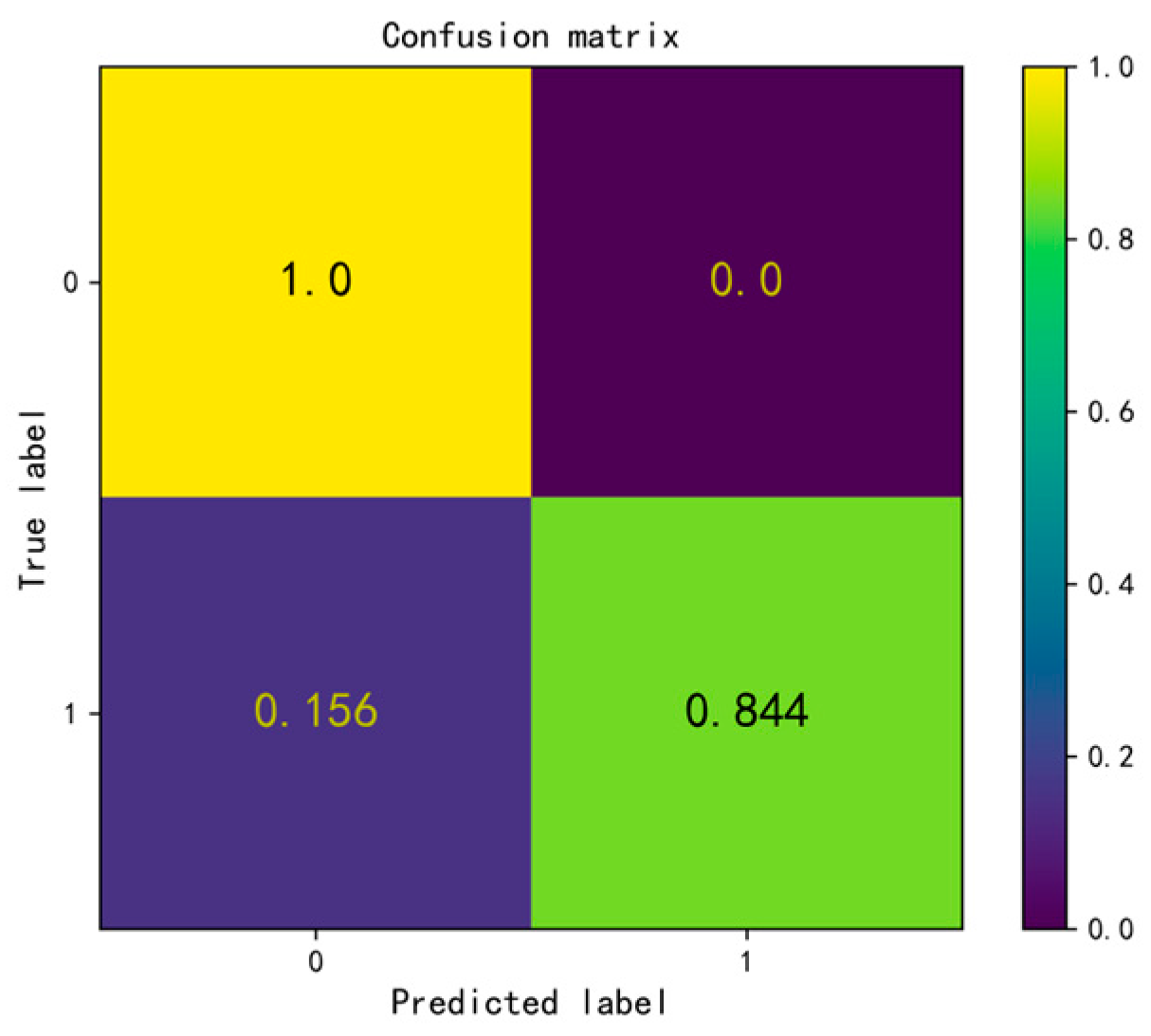
Then, the No. 24 hydrophone was used to analyze the test data and its confusion matrix diagram was obtained, as shown in Figure 28. Here, 84.4% of underwater sources were correctly classified, and 15.6% were incorrectly classified. The test accuracy of the No. 24 hydrophone was 0.844.
The above section only analyzed the data from the No. 24 hydrophone. In the next section, LightGBM is used to analyze data from all hydrophones with underwater source bandwidth. A threshold of 0.9 was manually set to determine whether the training was successful.
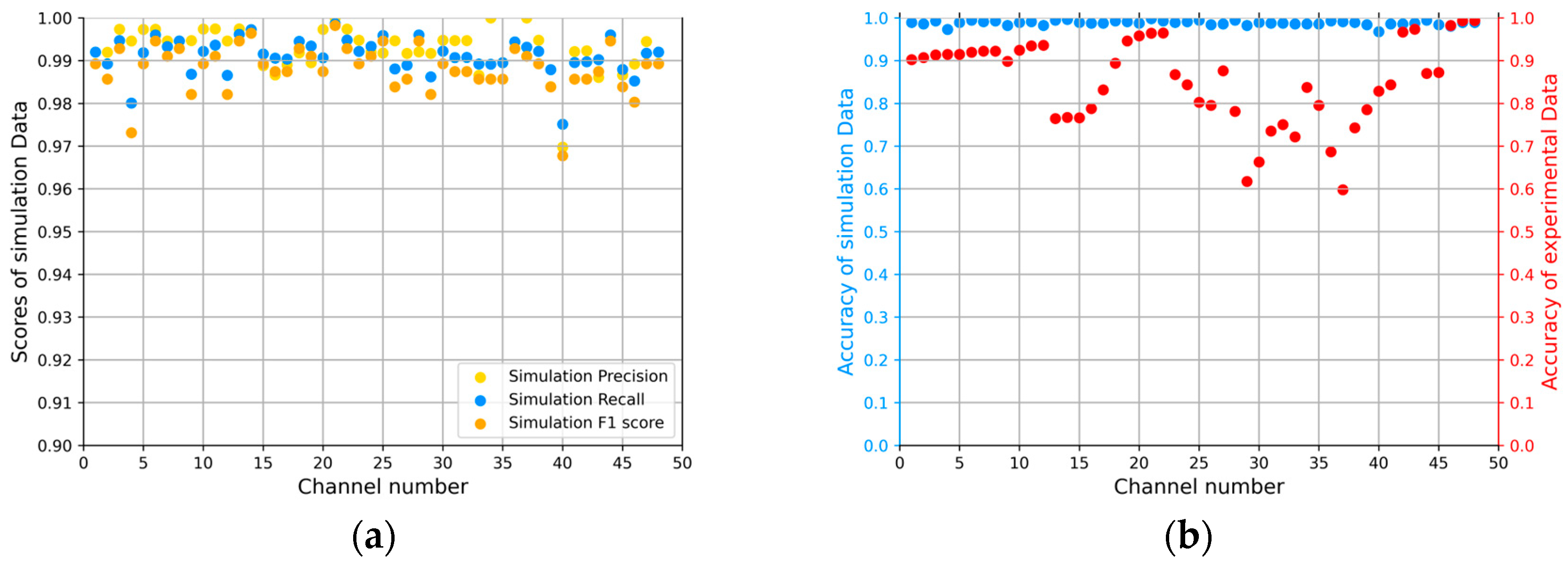
For underwater models using real and imaginary values as features, the training data for each hydrophone were a 2790 × 242 array, and the test data were a 1477 × 242 array. See Section 4.4 for details. The verification results of the simulation data of underwater targets characterized by real and imaginary values are shown in Figure 29a. The comparison diagram of the verification accuracy and test accuracy is shown in Figure 29b.
As can be seen from Figure 29, out of 48 hydrophones, the threshold of the simulation data reached 0.9, but only 20 hydrophones (numbered 1, 2, 3, 4, 5, 6, 7, 8, 10, 11, 12, 19, 20, 21, 22, 42, 43, 46, 47, 48) successfully reached the threshold of 0.9 when using experimental data.

5.3. Multi-Channel Joint Detection and Results Comparation

This section uses four models, namely, kNN, RS-kNN [1] (research was conducted and results obtained in the previous work), GBDT, and LightGBM, to compare a total of 16 models for two feature processing methods (modules, real and imaginary values), as well as for water surface target detection and underwater target detection. These models all analyzed and tested the performance of all 48 VLA hydrophones. The list of hydrophones whose surface target detection reached a threshold of 0.9 is shown in Table 6, and the list of hydrophones whose underwater target detection reached 0.9 is shown in Table 7.
For the two algorithms of kNN, there were 20 hydrophones that reached the threshold of 0.9 when using module features for kNN and 28 hydrophones that reached the threshold of 0.9 when using real and imaginary features; There were 25 hydrophones that reached the 0.9 threshold when RS-kNN used module features and 30 hydrophones that reached the 0.9 threshold when using real and imaginary value features. Both algorithms based on kNN reflect that using real and imaginary values could improve the passing rate of the hydrophone. This is due to the simplicity of the kNN algorithm itself, which requires more features to provide information in order to improve accuracy. In the best case, the two algorithms based on kNN used RS-kNN and used real values and imaginary values as features, and the number of hydrophones passing through was 30.
However, for the GBDT algorithm and the LightGBM algorithm, when the GBDT algorithm was characterized by modules, 41 hydrophones had a test accuracy higher than 0.9, whereas when using real and imaginary values as features, only 15 hydrophones had a test accuracy higher than 0.9. For the LightGBM model, when using modules as features, 40 hydrophones had a test accuracy higher than 0.9, whereas when using real and imaginary values as features, only 15 hydrophones had a test accuracy higher than 0.9. Both algorithms based on GBDT and LightGBM exhibited a higher pass rate for module features compared to real and imaginary value features because the features provided by the modules were sufficient for the algorithm to learn. The two algorithms achieved extremely high pass rates of 40 or even 41, respectively, which was even better than the best case (30 passes) of the two algorithms of kNN.
On the contrary, when using real and imaginary values as features, because the simple separation of real and imaginary values cannot reflect information that previously belonged to a single point, the features contained a lot of redundant information, making the features learned by the model unrepresentative to some extent and unable to make correct predictions.
For the two algorithms of kNN, there were 21 hydrophones that reached the threshold of 0.9 when using module features for kNN and 18 hydrophones that reached the threshold of 0.9 when using real and imaginary features. There were 31 hydrophones that reached the 0.9 threshold when using module features for RS-kNN and 40 hydrophones that reached the 0.9 threshold when using real and imaginary value features. Neither of the two algorithms based on kNN reflected better universality of using real and imaginary values or module features. In the best case, the two algorithms based on kNN used RS-kNN model and used real and imaginary values as features, and the number of hydrophones passing through was 40.
For the GBDT algorithm and LightGBM algorithm, when the GBDT algorithm was characterized by modules, 35 hydrophones had a test accuracy higher than 0.9, whereas when using real and imaginary values as features, 42 hydrophones had a test accuracy higher than 0.9. For the LightGBM algorithm, when using modules as the feature, 31 hydrophones had a test accuracy higher than 0.9, whereas when using real and imaginary values as the feature, only 20 hydrophones had a test accuracy higher than 0.9. Neither of the two algorithms based on GBDT and LightGBM reflected better universality of using real and imaginary values or module features. The best model was the GBDT algorithm characterized by real and imaginary values, and the number of hydrophones passing through was 42.

6. Conclusions and Discussion

In this article, a multi-channel joint detection method based on machine learning is proposed for S/U acoustic source recognition. From the entire process and the results of experiment, the following conclusions can be drawn:
(1)
The results of the No. 24 hydrophone using the GBDT model show that the training model established using simulation data effectively solved the problem of S/U acoustic source recognition. The ultimate optimal model also achieved a good balance and had good experimental accuracy.
(2)
Using LightGBM to classify the experimental data of hydrophone 24 achieved the best balance between precision and recall, with good experimental accuracy.
(3)
Four machine learning methods (kNN, RS-kNN, GBDT, and LightGBM) were used to identify all 48 hydrophones of the VLA for S/U acoustic source recognition. The results show that the recognition performance of GBDT and LightGBM was better than that of kNN when modules were used as features.
(4)
For surface models, two algorithms based on GBDT and LightGBM exhibited a higher pass rate for module features compared to real and imaginary value features because the features provided by the modules were sufficient for the algorithm to learn. The two algorithms achieved extremely high pass rates of 40 or even 41, respectively, which is even better than the best case (30 passes) of the two algorithms based on kNN and RS-kNN. On the contrary, when using real and imaginary values as features, because the simple separation of real and imaginary values cannot reflect information that previously belonged to a single point, the features contained a lot of redundant information, making the features learned by the model unrepresentative to some extent and unable to make correct predictions.
In this work, we did not consider the impact of array signals on improving experimental accuracy. Just like the article published by Witold [10] in 2021, using a covariance matrix to achieve target tracking is worth learning from. In the next step, we will consider using multiple hydrophones for joint detection to improve testing accuracy.

Author Contributions

Conceptualization, Q.Y. and W.Z.; methodology, Q.Y.; validation, Q.Y.; formal analysis, Q.Y.; investigation, Q.Y. and Y.L.; resources, M.Z., W.Z. and J.S.; data curation, M.Z. and W.Z.; writing—original draft, Q.Y.; writing—review and editing, M.Z., W.Z. and J.S. All authors have read and agreed to the published version of the manuscript.

Funding

This research received no external funding.

Institutional Review Board Statement

Not applicable.

Informed Consent Statement

Not applicable.

Data Availability Statement

The reader can ask for all the related data from the first author ([email protected]) and the corresponding author ([email protected]).

Acknowledgments

The authors would like to thank SPIB (http://spib.linse.ufsc.br/, accessed on 23 February 2022), where the related data originally come from.

Conflicts of Interest

The authors declare no conflict of interest.

References

  1. Zhang, W.; Wu, Y.; Shi, J.; Leng, H.; Zhao, Y.; Guo, J. Surface and Underwater Acoustic Source Discrimination Based on Machine Learning Using a Single Hydrophone. J. Mar. Sci. Eng. 2022, 10, 321. [Google Scholar] [CrossRef]
  2. Nicolas, B.; Mars, J.I.; Lacoume, J.-L. Source Depth Estimation Using a Horizontal Array by Matched-Mode Processing in the Frequency-Wavenumber Domain. EURASIP J. Adv. Signal Process. 2006, 2006, 065901. [Google Scholar] [CrossRef] [Green Version]
  3. Tolstoy, A. Matched Field Processing for Underwater Acoustics. In Matched Field Processing for Underwater Acoustics/Alexandra Tolstoy; World Scientific: Singapore, 1993. [Google Scholar]
  4. Wilson, G.R.; Koch, R.A.; Vidmar, P.J. Matched mode localization. J. Acoust. Soc. Am. 1988, 84, 310–320. [Google Scholar] [CrossRef]
  5. Westwood, E.K. Broadband matched-field source localization. J. Acoust. Soc. Am. 1992, 91, 2777–2789. [Google Scholar] [CrossRef]
  6. Baggeroer, A.B.; Kuperman, W.A.; Mikhalevsky, P.N. An overview of matched field methods in ocean acoustics %J Oceanic Engineering. IEEE J. Ocean. Eng. 1993, 18, 401–424. [Google Scholar] [CrossRef]
  7. Smith, G.B.; Feuillade, C.; Balzo, D.R.D.; Byrne, C.L. A nonlinear matched-field processor for detection and localization of a quiet source in a noisy shallow-water environment. J. Acoust. Soc. Am. 1989, 85, 1158–1166. [Google Scholar] [CrossRef]
  8. Michalopoulou, Z.-H.; Porter, M.B. Matched-field processing for broad-band source localization. IEEE J. Ocean. Eng. 1996, 21, 384–392. [Google Scholar] [CrossRef] [Green Version]
  9. Wawrzyniak, N.; Stateczny, A. MSIS Image Postioning in Port Areas with the Aid of Comparative Navigation Methods. Pol. Marit. Res. 2017, 24, 32–41. [Google Scholar] [CrossRef] [Green Version]
  10. Kazimierski, W.; Zaniewicz, G. Determination of Process Noise for Underwater Target Tracking with Forward Looking Sonar. Remote. Sens. 2021, 13, 1014. [Google Scholar] [CrossRef]
  11. Piskur, P.; Szymak, P. Algorithms for passive detection of moving vessels in marine environment. J. Mar. Eng. Technol. 2017, 16, 377–385. [Google Scholar] [CrossRef]
  12. Premus, V.E.; Helfrick, M.N. Use of mode subspace projections for depth discrimination with a horizontal line array: Theory and experimental results. J. Acoust. Soc. Am. 2013, 133, 4019–4031. [Google Scholar] [CrossRef]
  13. Porter, M.B. The KRAKEN Normal Mode Program; SACLANT Undersea Researeh Centre: La Spezia, Italy, 1991. [Google Scholar]
  14. Premus, V.E.; Backman, D. A Matched Subspace Approach to Depth Discrimination in a Shallow Water Waveguide. In Proceedings of the Conference Record of the Forty-First Asilomar Conference on Signals, Systems and Computers, Pacific Grove, CA, USA, 4–7 November 2007; Ocean Acoustical Services and Instrumentation Systems Inc.: Lexington, MA, USA, 2007. [Google Scholar]
  15. Yang, T.C. Data-based matched-mode source localization for a moving source. J. Acoust. Soc. Am. 2014, 135, 1218–1230. [Google Scholar] [CrossRef]
  16. Du, J.; Zheng, Y.; Wang, Z.; Cui, H.; Liu, Z. Passive Acoustic Source Depth Discrimination with Two Hydrophones in Shallow Water. In Proceedings of the OCEANS 2016—Shanghai, Shanghai, China, 10–13 April 2016. [Google Scholar]
  17. Conan, E.; Bonnel, J.; Chonavel, T.; Nicolas, B. Source depth discrimination with a vertical line array. J. Acoust. Soc. Am. 2016, 140, EL434–EL440. [Google Scholar] [CrossRef]
  18. Conan, E.; Bonnel, J.; Nicolas, B.; Chonavel, T. Using the trapped energy ratio for source depth discrimination with a horizontal line array: Theory and experimental results. J. Acoust. Soc. Am. 2017, 142, 2776–2786. [Google Scholar] [CrossRef]
  19. Liang, G.; Zhang, Y.; Zhang, G.; Feng, J.; Zheng, C. Depth Discrimination for Low-Frequency Sources Using a Horizontal Line Array of Acoustic Vector Sensors Based on Mode Extraction. Sensors 2018, 18, 3692. [Google Scholar] [CrossRef] [Green Version]
  20. Niu, H.; Reeves, E.; Gerstoft, P. Source localization in an ocean waveguide using supervised machine learning. J. Acoust. Soc. Am. 2017, 142, 1176–1188. [Google Scholar] [CrossRef]
  21. Niu, H.; Ozanich, E.; Gerstoft, P. Ship localization in Santa Barbara Channel using machine learning classifiers. J. Acoust. Soc. Am. 2017, 142, EL455–EL460. [Google Scholar] [CrossRef]
  22. Friedman, J.H. Greedy Function Approximation: A Gradient Boosting Machine. Ann. Stat. 2001, 29, 1189–1232. [Google Scholar] [CrossRef]
  23. Ke, G.; Meng, Q.; Finley, T. LightGBM: A Highly Efficient Gradient Boosting Decision Tree. In Proceedings of the 31st International Conference on Neural Information Processing Systems, Long Beach, CA, USA, 4–9 December 2017. [Google Scholar]
  24. Signal Processing Information Base (SPIB). Available online: http://spib.linse.ufsc.br/ (accessed on 10 October 2021).
  25. Gingras, D.F.; Gerstoft, P. Inversion for geometric and geoacoustic parameters in shallow water: Experimental results. J. Acoust. Soc. Am. 1995, 97, 34. [Google Scholar] [CrossRef]
  26. Krolik, L.J. The performance of matched-field beamformers with Mediterranean vertical array data. IEEE Trans. Signal Process. 1996, 44, 2605–2611. [Google Scholar] [CrossRef]
  27. Choi, J.; Choo, Y.; Lee, K. Acoustic Classification of Surface and Underwater Vessels in the Ocean Using Supervised Machine Learning. Sensors 2019, 19, 3492. [Google Scholar] [CrossRef] [PubMed] [Green Version]
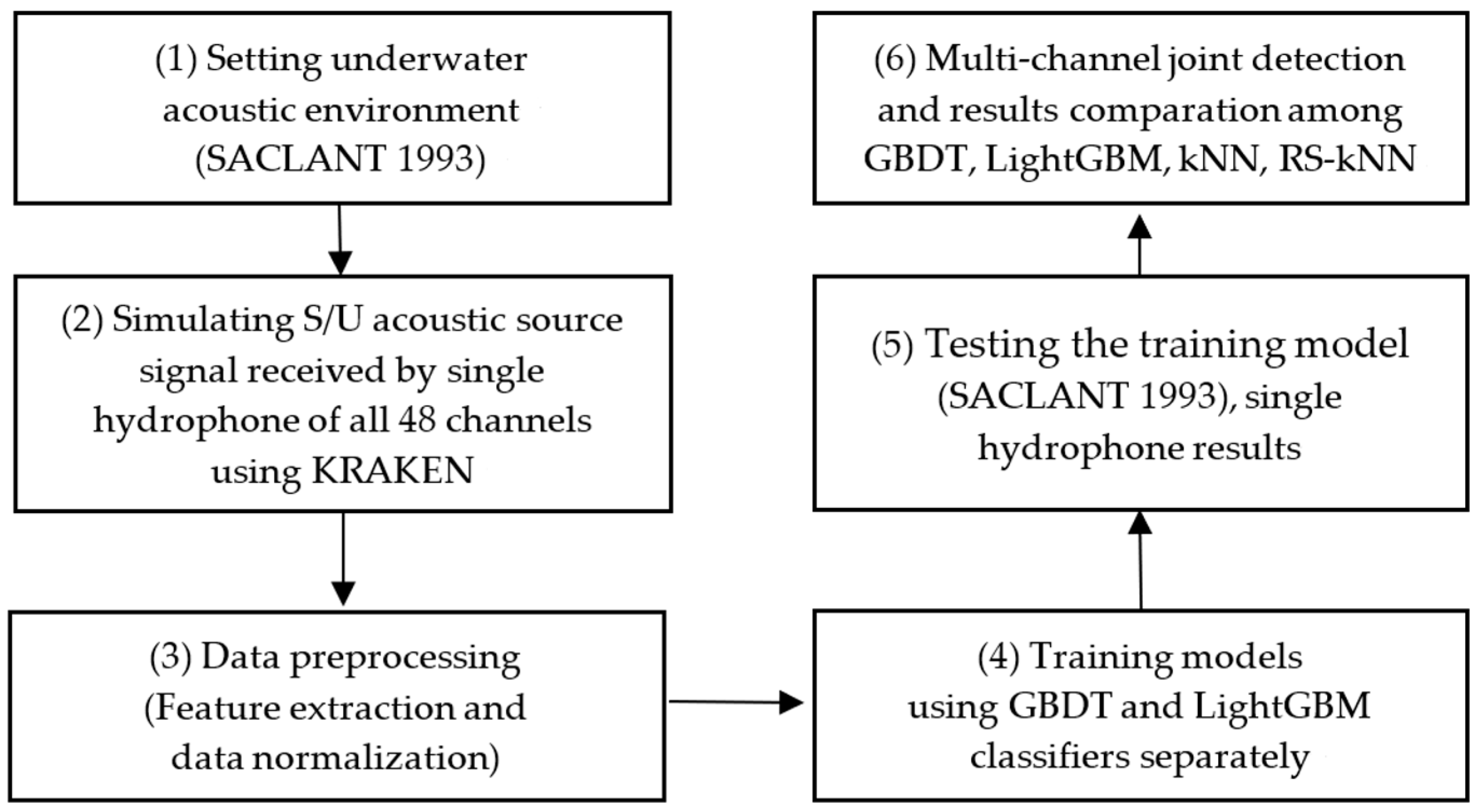
Figure 1. The overall architecture of S/U acoustic source recognition using the multi-channel joint detection method based on machine learning.
Jmse 11 01587 g001
Figure 2. The experimental environment of SACLANT 1993.
Jmse 11 01587 g002
Figure 3. (a) SNR of the surface source; (b) SNR of the underwater source.
Jmse 11 01587 g003
Figure 4. The spectrogram of the experimental data of hydrophone No. 24.
Jmse 11 01587 g004
Figure 5. The features of one sample of the experimental data, where the horizontal axis represents the frequency from 0 to 210 Hz and the vertical axis is the normalized amplitude from −1 to 1.
Jmse 11 01587 g005
Figure 6. (a) The confusion matrix diagram of the No. 24-GBDT-mod-surface model; (b) the ROC diagram of the No. 24-GBDT-mod-surface model.
Jmse 11 01587 g006
Figure 7. The confusion matrix diagram of the test data.
Jmse 11 01587 g007
Figure 8. (a) Verification results of simulation data; (b) comparison diagram of verification accuracy and test accuracy.
Jmse 11 01587 g008
Figure 9. (a) The confusion matrix diagram of the No. 24-GBDT-com-surface model; (b) the ROC diagram of the No. 24-GBDT-com-surface model.
Jmse 11 01587 g009
Figure 10. The confusion matrix diagram of the test data.
Jmse 11 01587 g010
Figure 11. (a) Verification results of simulation data; (b) comparison diagram of verification accuracy and test accuracy.
Jmse 11 01587 g011
Figure 12. (a) The confusion matrix diagram of the No. 24-GBDT-mod-underwater model; (b) the ROC diagram of the No. 24-GBDT-mod-underwater model.
Jmse 11 01587 g012
Figure 13. The confusion matrix diagram of the test data.
Jmse 11 01587 g013
Figure 14. (a) Verification results of simulation data; (b) comparison diagram of verification accuracy and test accuracy.
Jmse 11 01587 g014
Figure 15. (a) The confusion matrix diagram of the No. 24-GBDT-com-underwater model; (b) the ROC diagram of the No. 24-GBDT-com-underwater model.
Jmse 11 01587 g015
Figure 16. The confusion matrix diagram of the test data.
Jmse 11 01587 g016
Figure 17. (a) Verification results of simulation data; (b) comparison diagram of verification accuracy and test accuracy.
Jmse 11 01587 g017
Figure 18. (a) The confusion matrix diagram of the No. 24-LightGBM-mod-surface model; (b) the ROC diagram of the No. 24-LightGBM-mod-surface model.
Jmse 11 01587 g018
Figure 19. The confusion matrix diagram of the test data.
Jmse 11 01587 g019
Figure 20. (a) Verification results of simulation data; (b) comparison diagram of verification accuracy and test accuracy.
Jmse 11 01587 g020
Figure 21. (a) The confusion matrix diagram of the No. 24-LightGBM-com-surface model; (b) the ROC diagram of the No. 24-LightGBM-com-surface model.
Jmse 11 01587 g021
Figure 22. The confusion matrix diagram of the test data.
Jmse 11 01587 g022
Figure 23. (a) Verification results of simulation data; (b) comparison diagram of verification accuracy and test accuracy.
Jmse 11 01587 g023
Figure 24. (a) The confusion matrix diagram of the No. 24-LightGBM-mod-underwater model; (b) the ROC diagram of the No. 24-LightGBM-mod-underwater model.
Jmse 11 01587 g024
Figure 25. The confusion matrix diagram of the test data.
Jmse 11 01587 g025
Figure 26. (a) Verification results of simulation data; (b) comparison diagram of verification accuracy and test accuracy.
Jmse 11 01587 g026
Figure 27. (a) The confusion matrix diagram of the No. 24-LightGBM-com-underwater model; (b) the ROC diagram of the No. 24-LightGBM-com-underwater model.
Jmse 11 01587 g027
Figure 28. The confusion matrix diagram of the test data.
Jmse 11 01587 g028
Figure 29. (a) Verification results of simulation data; (b) comparison diagram of verification accuracy and test accuracy.
Jmse 11 01587 g029
Table 1. The experimental environment information of SACLANT 1993.
Depth of the top hydrophone 18.7 m
Depth of the bottom hydrophone 112.7 m
The space of the VLA 2 m
The number of the VLA 48
Depth of source 69 m
Range of source 5.9~6.9 km
Surface target frequency band 20~72 Hz
Underwater target frequency band 170~220 Hz
Table 2. Results of simulation data from No. 24 hydrophone (precision, recall, F1, and accuracy).
PrecisionRecallF1 ScoreAccuracy
Modules0.99420.98850.99130.9946
Real and
imaginary values
0.98920.97860.98390.9892
Table 3. Results of simulation data from No. 24 hydrophone (precision, recall, F1, and accuracy).
PrecisionRecallF1 ScoreAccuracy
Modules0.976910.98830.9839
Real and
imaginary values
0.99180.99160.99180.9892
Table 4. Results of simulation data from No. 24 hydrophone (precision, recall, F1, and accuracy).
PrecisionRecallF1 ScoreAccuracy
Modules0.98680.99730.99210.9892
Real and
imaginary values
10.99470.99740.9964
Table 5. Results of simulation data from No. 24 hydrophone (precision, recall, F1, and accuracy).
PrecisionRecallF1 ScoreAccuracy
Modules0.94890.99200.96990.9588
Real and
imaginary values
0.99470.99200.99330.9910
Table 6. List of hydrophones successfully reaching 0.9 for water surface target detection.
Machine
Learning Method
FeatureList of Hydrophones That Reached the ThresholdNumber of
Hydrophones
That Reached
Threshold
kNNModules15, 16, 17, 18, 19, 20, 21, 22, 23, 24,
25, 26, 27, 28, 29, 34, 36, 37, 38, 39
20
Real and
imaginary
values
16, 17, 18, 19, 20, 21, 22, 23, 26,
27, 28, 29, 30, 31, 32, 33, 34, 35, 36,
37, 38, 39, 40, 41, 42, 43, 47, 48
28
RS-kNNModules15, 16, 17, 18, 19, 20, 21, 22, 23, 24,
25, 26, 27, 28, 29, 30, 31, 32, 33, 34,
35, 36, 37, 38, 39
25
Real and
imaginary
values
16, 17, 18, 19, 20, 21, 22, 23, 24, 25,
26, 27, 28, 29, 30, 31, 32, 33, 34, 35,
36, 37, 38, 39, 40, 41, 42, 46, 47, 48
30
GBDTModules1, 2, 3, 4, 5, 6, 7, 8, 9, 10, 11, 12, 13, 14, 15, 16, 17, 18, 19, 20, 21, 22, 23,
24, 26, 27, 28, 29, 30, 31, 32, 33, 34,
35, 36, 37, 38, 39, 40, 44, 45
41
Real and
imaginary
values
30, 31, 32, 33, 34, 35, 36, 37, 38,
39, 40, 41, 42, 43, 44
15
LightGBMModules1, 2, 3, 4, 5, 6, 7, 8, 9, 10, 11, 12, 13, 14, 15, 16, 17, 18, 19, 20, 21, 22, 23, 24, 25, 26, 27, 28, 29, 30, 32, 33, 34, 35, 36, 37, 38, 39, 44, 4540
Real and
imaginary
values
30, 31, 32, 33, 34, 35, 36, 37, 38,
39, 40, 41, 42, 43, 44
15
Table 7. List of hydrophones successfully reaching 0.9 for underwater target detection.
Machine
Learning Method
FeatureList of Hydrophones That Reached the ThresholdNumber of
Hydrophones
That Reached
the Threshold
kNNModules1, 2, 3, 4, 5, 6, 7, 8, 9, 10,
11, 12, 19, 20, 32, 33, 43, 45,
46, 47, 48
21
Real and
imaginary
values
4, 5, 6, 7, 8, 9, 10, 11, 19,
20, 32, 33, 41, 42, 43, 44, 46, 47
18
RS-kNNModules1, 2, 3, 4, 5, 6, 7, 8, 9, 10, 11, 12, 13, 14, 19, 20, 21, 23, 24, 32, 33, 34, 39,
41, 42, 43, 44, 45, 46, 47, 48
31
Real and
imaginary
values
1, 2, 3, 4, 5, 6, 7, 8, 9, 10,11, 12, 13,
14, 18, 19, 20, 21, 22, 23, 24, 25, 26,
27, 28, 31, 32, 33, 34, 35, 39, 40, 41,
42, 43, 44, 45, 46, 47, 48
40
GBDTModules1, 2, 3, 4, 5, 6, 7, 8, 9, 10, 11, 12, 13, 19, 20, 21, 22, 23, 24, 25, 26,
27, 32, 33, 34, 35, 39, 40, 41, 42,
43, 45, 46, 47, 48
35
Real and
imaginary
values
1, 2, 3, 4, 5, 6, 7, 8, 9, 10, 11, 12, 13, 14, 15, 16, 17, 18, 19, 20, 21,
22, 23, 24, 25, 26, 27, 28, 33, 34,
35, 38, 39, 40, 41, 42, 43, 44, 45,
46, 47, 48
42
LightGBMModules1, 2, 3, 4, 5, 6, 7, 8, 9, 10, 11, 12, 19, 20, 21, 23, 24, 25, 27, 32, 33, 34, 35,
39, 41, 42, 43, 45, 46, 47, 48
31
Real and
imaginary
values
1, 2, 3, 4, 5, 6, 7, 8, 10, 11, 12, 19, 20, 21, 22, 42, 43, 46, 47, 4820
Disclaimer/Publisher’s Note: The statements, opinions and data contained in all publications are solely those of the individual author(s) and contributor(s) and not of MDPI and/or the editor(s). MDPI and/or the editor(s) disclaim responsibility for any injury to people or property resulting from any ideas, methods, instructions or products referred to in the content.