Article

Research on Multi-Target Path Planning for UUV Based on Estimated Path Cost

School of Electrical Engineering, Naval University of Engineering; Wuhan 430030, China
*
Author to whom correspondence should be addressed.
J. Mar. Sci. Eng. 2023, 11(8), 1582; https://doi.org/10.3390/jmse11081582
Submission received: 30 June 2023 / Revised: 2 August 2023 / Accepted: 8 August 2023 / Published: 12 August 2023
(This article belongs to the Special Issue AI for Navigation and Path Planning of Marine Vehicles)

Abstract

:
The precision and efficiency of multi-target path planning are crucial factors influencing the performance of anti-mine operations using unmanned underwater vehicles (UUVs). Addressing the inadequacies in computation time and solution quality present in existing path planning algorithms, this study proposes a novel path cost estimation strategy based on neural networks. This strategy swiftly generates an accurate cost matrix, ensuring the attainment of high-quality traversal orders when utilized as input for the traveling salesman problem, thereby yielding a globally optimal path. Simulation experiments demonstrate that while maintaining high-quality solutions, the proposed strategy significantly enhances the computational efficiency of the algorithm. Furthermore, the practical application and effectiveness of the proposed algorithm have been demonstrated through an actual UUV prototype experiment in a lake environment.

1. Introduction

Unmanned underwater vehicles (UUVs), recognized for their distinctive attributes of stealth and flexibility, have been widely adopted in various military operations [1]. Utilizing UUVs for automating anti-mine activities has emerged as a significant progression to minimize the threat that sea mines pose to surface warships and submarines [2]. Path planning technology, a crucial facet of autonomous navigation, plays a pivotal role in assuring safe operation of UUVs [3]. A special focus within this realm is multi-target path planning, which involves formulating a collision-free optimal trajectory, initiating from the starting point and traversing all designated target points within an environment laden with obstacles [4,5].
Many researchers have transformed the multi-target path planning problem into the traveling salesman problem (TSP) [6]. Consequently, the solution to multi-target path planning problems can be summarized as follows: construct a path cost matrix; solve TSP with known path cost and obtain the traversal order of each target point; plan the global optimal path in order.
Minghao L et al. [7] utilized a bidirectional dynamic weighted-A star (BD-A*) algorithm to plan the shortest path between arbitrary pairs of target points, thereby constructing an actual path cost matrix. Subsequently, a learn memory-swap sequence particle swarm optimization (LM-SSPSO) algorithm was employed to address the TSP, thus determining the shortest path encompassing visiting all target points. However, this methodology could not circumvent the necessity for path planning between any two points, resulting in considerable computational burden. In contrast, Daichuan Y et al. [8] proposed a distinctive multi-target path planning algorithm, combining the ant colony optimization technique with an enhanced Probabilistic Roadmap Method (PRM). In their approach, the Euclidean distance between each pair of target points was adopted as the path cost. Following the acquisition of this cost matrix, the ant colony algorithm determined the traversal order, and finally, the PRM algorithm planned the path between each target point, adhering to this order. Nonetheless, the cost matrix, constructed based on Euclidean distance in this method, cannot ensure the optimality of the path.
Wenjun Y et al. [9] put forth a multi-target path planning algorithm, combining the merits of Rapidly-exploring Random Trees (RRT) and ant colony optimization techniques. This innovative method introduced the Euclidean distance cost matrix into the ant colony algorithm, generating an iterative solution. Throughout the iteration process, the RRT algorithm was invoked to update the cost of paths with a pheromone level surpassing a defined threshold value. Upon the conclusion of an iteration, the RRT algorithm refreshed the cost of all segments within the solution path. Upon reaching the maximum permitted iterations, the solution offering the least total path cost was selected as the optimal solution. Despite this method yielding a relatively superior solution, the number of actual planning executions for RRT escalated with increased iterations, inducing a linear surge in the algorithm’s execution time.
Aiming at the multi-target path planning problem of unmanned cruise ship collecting water samples in complex waters, Jiabin Y et al. [10] constructed a two-dimensional environment map by grid method. In the Grey Wolf Optimization (GWO) algorithm [11], the environmental impact factors are introduced into the fitness function to reflect the impact of obstacles and unknown areas on multi-target sequence planning. However, it is difficult to theoretically prove the advantages of this method compared to using Euclidean distance cost matrix alone to solve TSP. Finally, a method combining A* algorithm and artificial potential fields (APF) was used to plan the global path.
At present, there are also studies combining the task allocation of UUV clusters [12] and route planning in dynamic environments [13] into TSP. However, both of them directly use the Euclidean distance between two points as the path cost, ignoring the importance of the actual path cost in solving TSP in the presence of obstacles.
To address these issues, a novel strategy based on neural network for estimating path costs is proposed in this paper. The core strength of this strategy lies in its capability to construct precise cost matrices efficiently. When this cost matrix is used as an input for the TSP, the generated solution set is assured to contain high-quality traversal orders, leading to the realization of globally optimal path planning. Importantly, while maintaining solution quality, our strategy greatly enhances computation efficiency, offering an innovative and efficient method for high-dimensional, multi-target path planning.
The innovative contributions of this paper can be summarized as follows.
  • Transform the path planning problem of a mine countermeasures UUV dealing with multiple ground mines into a TSP.
  • Train a neural network for estimating path costs, quickly creating a cost matrix that accurately reflects the shortest path between two target points.
  • During the global path planning process, an initial check is performed to see if the direct line segment between two points intersects any obstacles. If there is no intersection, the segment is considered as the feasible path, with its Euclidean distance serving as the path cost.
The remaining of this paper is organized as follows. Section 2 introduces the environmental modeling and the constraints inherent in UUV navigation tasks. The principles and methodologies of multi-target path planning and the training process for the neural network aimed at path cost estimation are thoroughly expounded in Section 3. Section 4 is devoted to constructing three variants of cost matrices and the application of a genetic algorithm in solving the TSP for globally optimal path planning, followed by an analysis of the efficiency and time cost of the proposed method. In Section 5, we confirm the feasibility of our proposed algorithm by conducting field trials with a UUV in a lake environment. The conclusion and future work are discussed in Section 6.

2. Examination and Analysis of the Problem

Information on obstacles and suspected target points in the mission sea area have been obtained by other reconnaissance methods. Considering that UUVs often operate at a fixed depth underwater in real scenarios, this study simplifies the path planning problem for mine countermeasure UUVs dealing with multiple ground mines, establishing a two-dimensional feature map to abstractly represent the mission sea area. The feature map displays the starting point (green point), suspected target points (red points), and obstacle circles (black circles) of the UUV entering the mission sea area, along with their size information in the global coordinate system. The obstacle circles are circular expansions based on the circumscribed circles of irregular polygonal obstacles, with an expansion radius Rp equivalent to the UUV’s width. According to the above rules, two task scenarios are constructed as shown in Figure 1.
In the feature map, the UUV can be considered as a point mass, with obstacle avoidance constraints as follows:
| | P u P k | | R k
In Equation (1), P u represents the coordinates of the UUV at any position along the path, P k signifies the coordinates of the center of the k-th obstacle circle, and R k denotes the radius of the k-th obstacle circle.
Given the certain false alarm rate of suspected targets, the UUV first inspects the suspected targets, confirms them as real ground mines, and then commences disposal operations. The operational constraints are as follows:
| | P u P i | | R h R s
In Equation (2), P i denotes the coordinates of the i-th suspected target point, R h represents the disposal operation radius, and R s signifies the sweep operation radius. Below is an illustrative diagram depicting the UUV avoiding obstacles and entering the operational radius (Figure 2):
In the process of global path planning, the veracity of suspected targets is inherently uncertain; thus, the constraints of UUV operation are not considered. Instead, the UUV is directed to reach the actual coordinates of the suspected targets. This study is focused on devising a closed path characterized by the least total path cost. It initiates from the origin, navigates around obstacles, traverses all suspected target points in a suitable order, and finally returns to the starting point. Here is the mathematical description of this concept.
min T o t a l _ P a t h _ C o s t = i = 1 n + 1 d i
In Equation (3), d i represents the cost of the i-th segment in the global closed path.

3. Estimated Path Cost-Based Multi-Target Path Planning Method

3.1. Algorithm Framework

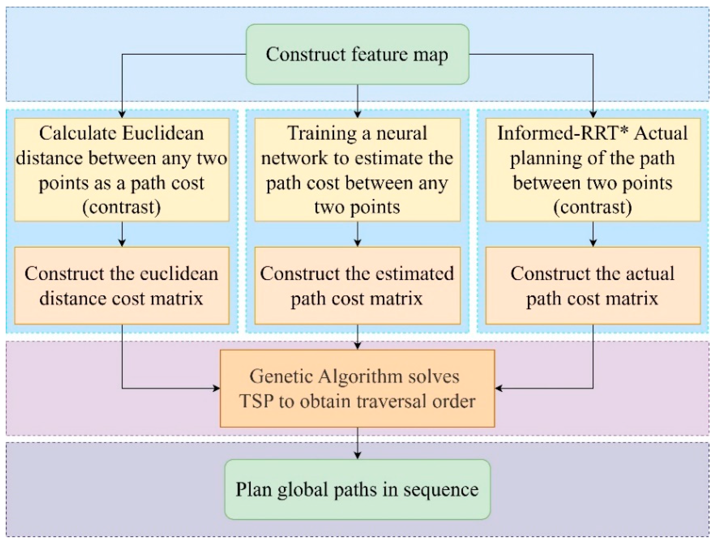
In this study, for the stage of constructing the path cost matrix, we have trained a path cost estimation neural network to estimate the cost of the path planned by the Informed-RRT* algorithm in an obstacle environment. The comparison experiments with the actual path cost matrix input and the Euclidean distance cost matrix indicate that this method improves the speed and accuracy of calculating the path cost matrix, providing a new approach to enhance the efficiency of the multi-target path planning algorithm. The overall framework of the algorithm is as follows (Figure 3).

3.2. Informed-RRT* Algorithm

The Informed-RRT* algorithm is an improvement of the RRT* algorithm [14]. It inherits the asymptotic optimality of the RRT* algorithm, and has strong search capability and fast planning speed. It replaces the global uniform sampling with elliptical sampling, effectively improving the sampling efficiency [15]. The flowchart of the Informed-RRT* algorithm is shown in Figure 4. In the first iteration of the Informed-RRT* algorithm, the cost of the path obtained by the global uniform sampling of the RRT* algorithm is used as the long axis length, the starting point and the target point are the foci, and the Euclidean distance between the two points is the focus distance, forming the original elliptical sampling area. Subsequent iterations are planned within the original elliptical sampling area. If a shorter path is obtained, the path cost currently updates the length of the ellipse’s long axis, resulting in an elliptical sampling area with a larger eccentricity and smaller area. The iteration continues in the updated ellipse until the maximum number of iterations is reached.
Experiments have shown that the path planned by the Informed-RRT* algorithm can approximate the optimal path and maintain stability. Features can be easily summarized from the related parameters, providing a basis for subsequent training of the estimation neural network model.

3.3. Path Cost Estimation Neural Network

3.3.1. Dataset Creation

Suppose that the line connecting the start point and target point intersects with m obstacle circles. Based on the value of m, datasets are created correspondingly. For example, in the case of m = 1, as depicted in Figure 5a, the sampling ellipse area is obtained by calculating the ellipse with the left focal point at the origin and the right focal point on the positive half-axis of the x-axis, followed by a series of rotations and translations. To facilitate parameter adjustment, the origin can be fixed at the origin, and the target point can be set on the x-axis, as illustrated in Figure 5b. Through multiple nested loops, parameters such as the coordinates of the center of the obstacle circle, the radius of the circle, and the horizontal coordinates of the target point are altered in certain steps, simulating various scenarios where the planned path avoids the obstacle circle.
Characterizing parameters from each scenario are used as inputs. These include the length of the line segment connecting the starting point and the target point, the height of the arc formed by the intersection of the line segment and the obstacle circle, the normalized distance from the perpendicular point of the arc height to the midpoint of the line segment, etc. In each scenario, the Informed-RRT* algorithm is invoked to obtain the actual cost of the planned path. To avoid randomness, the planning is repeated three times, and the average value of these three instances is taken as the output for that scenario. The inputs and outputs from all scenarios form into a dataset for training.
In the special case where m = 0, denoting that the line segment does not intersect any obstacle circles, a substantial number of experiments consistently demonstrate that the Informed-RRT* algorithm plans a straight or near-straight path. Therefore, it is feasible to directly output the Euclidean distance of this segment without neural network training. The corresponding calculation formula is as follows.
d = ( x 1 x 2 ) 2 + ( y 1 y 2 ) 2
In Equation (4), d signifies the path cost, where ( x 1 , y 1 ) and ( x 2 , y 2 ) , respectively, represent the coordinates of the start and end points for the planning instance.

3.3.2. Neural Network Training

A fully connected neural network with 5 layers and a total of 116 neurons, utilizing the ReLU activation function, mean squared error loss function, and the Adam optimizer is constructed. The dataset is shuffled and divided into a training set and a testing set for network training and testing, respectively. After training is completed, network parameters are saved and, following the neural network calculation rules, encapsulated into a function for future use.

3.4. Construction of the Path Cost Matrix

For the distribution of obstacles and target points in the two task scenarios shown in Figure 1, the following three types of path cost matrices are calculated, respectively, for comparison experiments.

3.4.1. Estimated Path Cost Matrix

The construction of the estimated path cost matrix is divided into two steps: First, calculate the characterization parameters for network input. Second, for any direct line segment between two target points, judge the distance from each obstacle circle center to the line segment one by one. For example, when a line segment intersects with a single obstacle, as shown in Figure 6.
The specific operation steps are as follows: Input the starting point V ( x v , y v ) and target point W ( x w , y w ) ; the center of the obstacle circle is denoted by O ( x o , y o ) and its radius by r. We then define P ( x p , y p ) as the point perpendicular to line segment VW from point O, and M ( x m , y m ) as the midpoint of the line segment VW. The calculation is done through vector Equation (5).
V O V W | V W | 2 = | V O | | V W | cos α | V W | 2 = | V P | | V W | = k
The ratio k of | V P | to | V W | is computed, and according to the principle of similar triangles, the computation for Equation (6) is as follows.
x p = x v + k ( x w x v ) y p = y v + k ( y w y v )
The coordinates of point P, denoted as ( x p , y p ) , can be determined. By examining the coordinates of points O and P, we can compute the distance | O P | between them. If | O P | < r , it signifies that line segment VW intersects with this obstacle circle.
For intersecting obstacle circles, further calculations are made to determine the height of the bow-shaped structure formed by the major arc and inferior arc intersecting with the line segment, as well as the normalized distance from the perpendicular point of the bow height to the midpoint of the line segment. The formulas to calculate the bow height of the structure formed by the major arc and inferior arc are as follows.
h ma = r + | O P | h ia = r | O P |
In Equation (7), h ma , h ia represents the bow heights formed by the major arc and the inferior arc. Further, the position of the obstacle circle center to the left or right of vector V W is determined through a vector cross-product operation, as follows: If V O × V W > 0 , it indicates that the center of the obstacle circle is to the left of vector V W , and thus the bow height h 11 on the left side of the line segment VW is h ma . If V O × V W = 0 , it means that the center of the obstacle circle falls on the line segment, and the bow heights on both sides are the radius r of the circle. If V O × V W < 0 , it suggests that the center of the obstacle circle is to the right of vector V W , so the bow height h 11 on the left of the vector V W is h ia .
The calculation formula of the normalized distance from the bow height to the midpoint of the line segment is as follows.
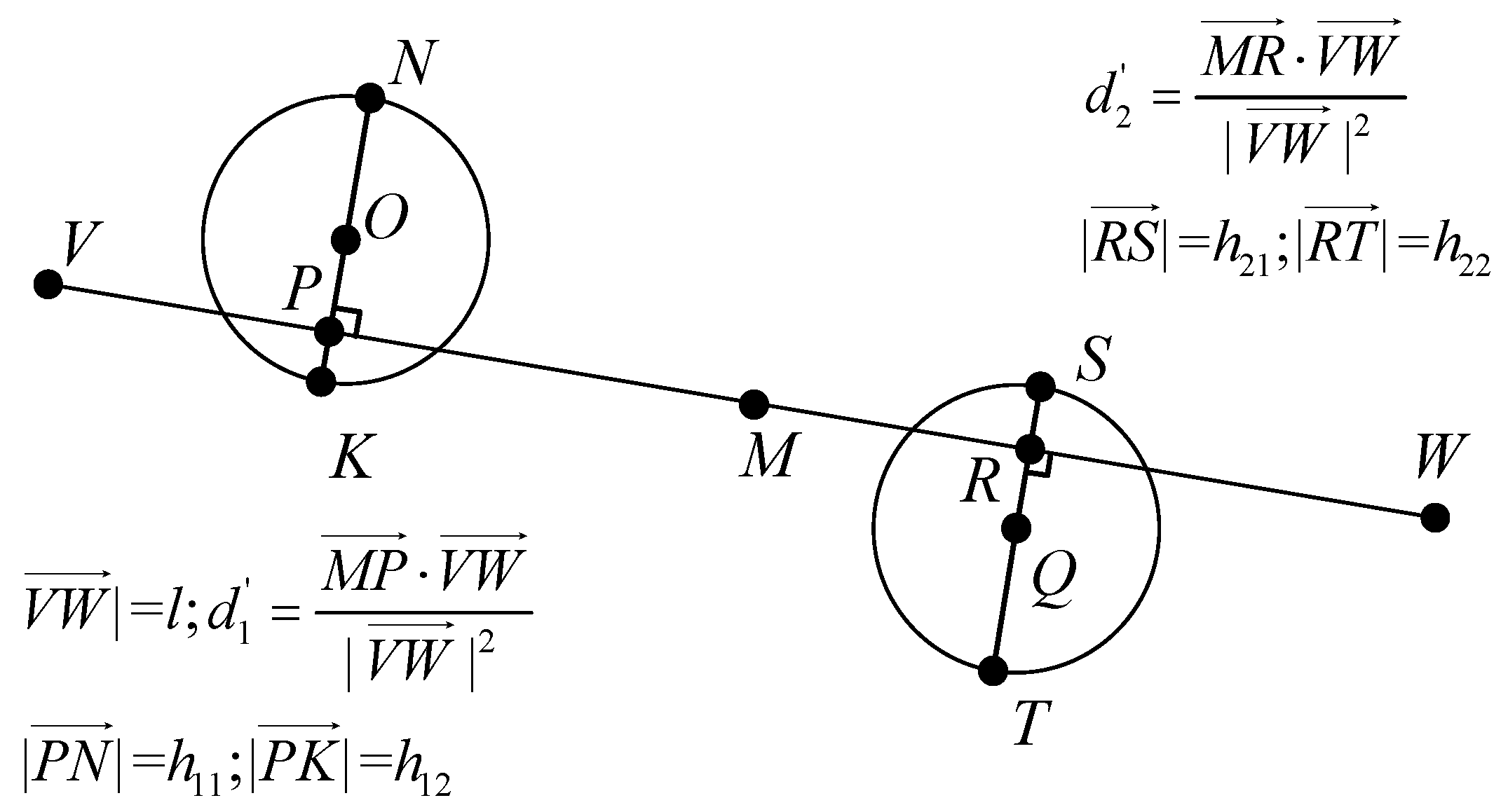
d = M P V W | V W | 2
In the second step, the corresponding network is selected based on m, and the estimated path cost is computed.
In situations where m = 1 , we input the following parameters in sequence: the segment length l , the normalized distance d from the obstacle circle, and the height h 11 , h 12 of the arc created by the intersection of the segment and the obstacle circle on both sides, as represented in Figure 6. In instances where m = 2 , we sequentially input these parameters: the segment length l , the normalized distance d 1 from the first obstacle circle, the height h 11 , h 12 of the arc created by the intersection of segment VW and the first obstacle circle on either side, the normalized distance d 2 from the second obstacle circle, and the height h 21 , h 22 of the arc formed by the intersection of the second obstacle circle on either side of the segment, as shown in Figure 7.
Upon calculating the estimated cost for all paths, construct the estimated path cost matrices D e s and D e s for task scenarios A and B, respectively, as D e s indicated in Equation (9).
D e s = 0 d 01 d 0 n d 10 0 d 1 n d n 0 d n 1 0
In Equation (9), D e s refers to the ( n + 1 ) order square matrix, while d i j ( i , j = 0 , 1 , , n ) signifies the estimated path cost between the i-th and the j-th point.

3.4.2. Actual Path Cost Matrix

In task scenarios A and B, the path between any two points is determined using the Informed-RRT* algorithm. Based on the results of this path planning, actual path cost matrices D r e and D r e are constructed.

3.4.3. Euclidean Distance Cost Matrix

This section uses Equation (4) to calculate the Euclidean distance between any two points and constructs the sum of the Euclidean distance cost matrix.

3.5. Genetic Algorithm for Solving the TSP

Currently, the main algorithms for solving the TSP include the Guo Tao algorithm [16], simulated annealing algorithm [17,18,19], ant colony algorithm [20,21], etc. Genetic algorithm [22] can escape from local optima through mutation operator, showing strong reliability. In this algorithm, the integer represents the gene coding from the starting point to the i-th target point. The order of traversing the target points corresponds one-to-one with the gene order of the chromosome. The total path cost of the traversal order represented by each chromosome serves as the fitness function. The smaller the total path cost, the higher the fitness. By setting parameters such as population size, iteration times, crossover probability, mutation probability, etc., the initial population is randomly generated, the fitness of individuals in the population is calculated, individuals with low fitness are eliminated, and the highest fitness individuals are cloned to fill the population. After performing chromosome crossover, mutation, and other operations on the new population individuals with a certain probability, an iteration is completed. This process is repeated until the maximum number of iterations is reached. The individual with the highest fitness is output, and the optimal traversal order is obtained. The algorithm flowchart is as follows (Figure 8).

4. Simulation Experiment and Analysis

4.1. Estimation Error Analysis

4.1.1. Error Analysis in Test Sets

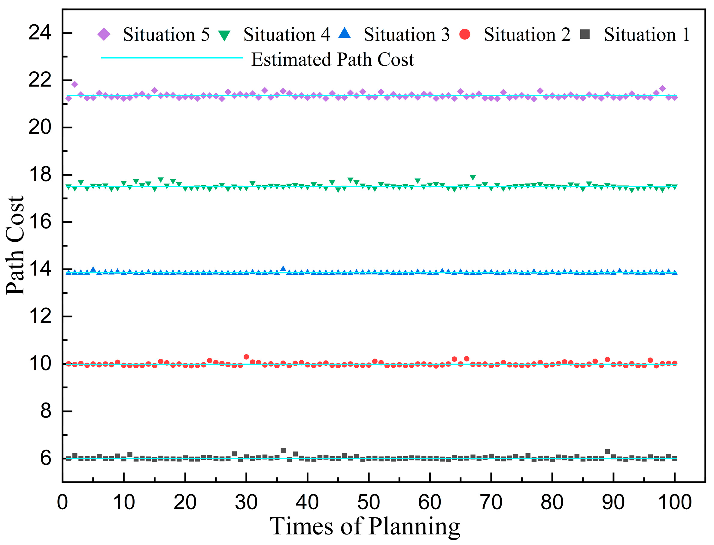
Due to the sampling principle of the Informed-RRT* algorithm, multiple planning results under the same scenario have a degree of uncertainty. In contrast, the trained network gives a constant output for a given input. To verify the reliability of the path cost estimation neural network, five scenarios were randomly selected from the test set. In each scenario, the Informed-RRT* algorithm was invoked to plan 100 times, and the actual path costs were recorded. These were then compared with their path cost estimates, as shown in Figure 9.
Quantitatively, the absolute mean error, root mean square error between the actual and estimated path costs, and the distribution of points above and below the estimated path cost line for each group are shown in Table 1.
As shown in Table 1, the actual path cost values are scattered evenly on both sides of the estimated value line in all scenarios, and the maximum absolute average percentage error in the five situations is only 0.684%, demonstrating the accuracy of the path cost estimation neural network.

4.1.2. Error Analysis of Estimating Path Cost Matrix

To ascertain the accuracy of the estimated path cost, we resort to the given Equation (10).
i = 0 n 1 j = i + 1 n d i j d i j + j = 0 n 1 i = j + 1 n d i j d i j ( n 2 + n + 1 ) d i j
In Equation (10), d i j ( i , j = 0 , 1 , , n ) represents the actual path cost from the i-th point to the j-th point, as planned by the Informed-RRT* algorithm. After calculation, the absolute average percentage errors of the estimated path cost matrix and the actual path cost matrix in the two task scenarios are 0.324% and 0.297%, respectively, further demonstrating the accuracy of the estimated path cost.

4.2. Solve the Traversal Order

The three cost matrices from Section 3.4 are separately input into the TSP and solved using a genetic algorithm. The number and distribution of obstacles and target points in the two task scenarios are different. Reasonable parameter settings have been experimentally tested and the algorithm parameters are shown in Table 2.
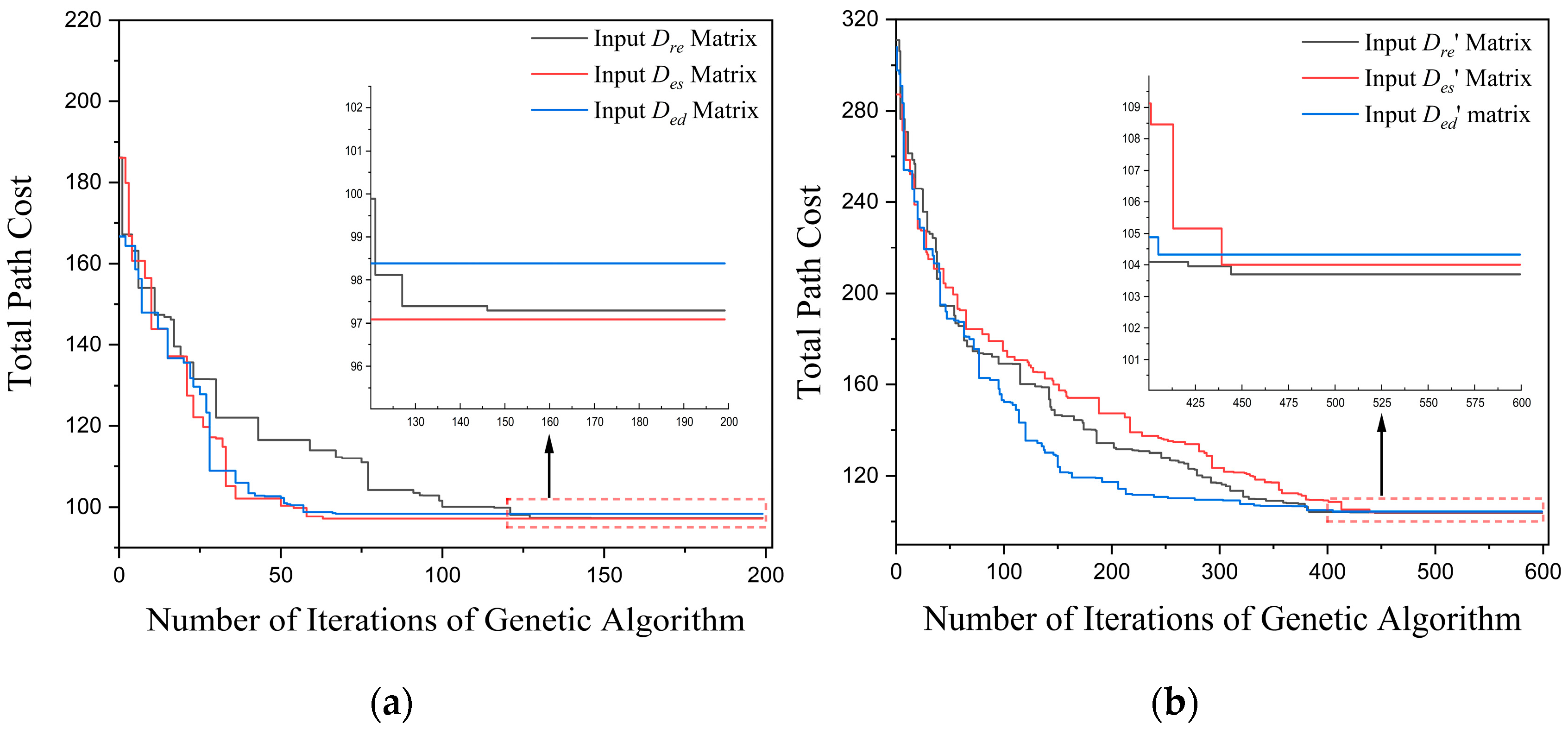
For task scenarios A and B, input three types of cost matrices, respectively, and use the genetic algorithm to solve the TSP to obtain the traversal order that minimizes the total path cost; the iteration process of the genetic algorithm is shown in Figure 10.
The results show that the genetic algorithm can quickly converge when inputting three types of cost matrices. In scenario A, the best traversal orders obtained from inputting D r e and D e s are the same and are set as order 1; in scenario B, the best traversal orders obtained from inputting D r e and D e s are also the same and are set as order 3, further verifying the feasibility of the estimated path cost method. It is worth noting that the total path cost obtained at this time is obtained based on their respective input cost matrices, so even if the same traversal order is obtained, the final convergence result of the total path cost still has a slight deviation. The total path cost corresponding to the obtained traversal order should be subject to the global planning result.

4.3. Global Path Planning

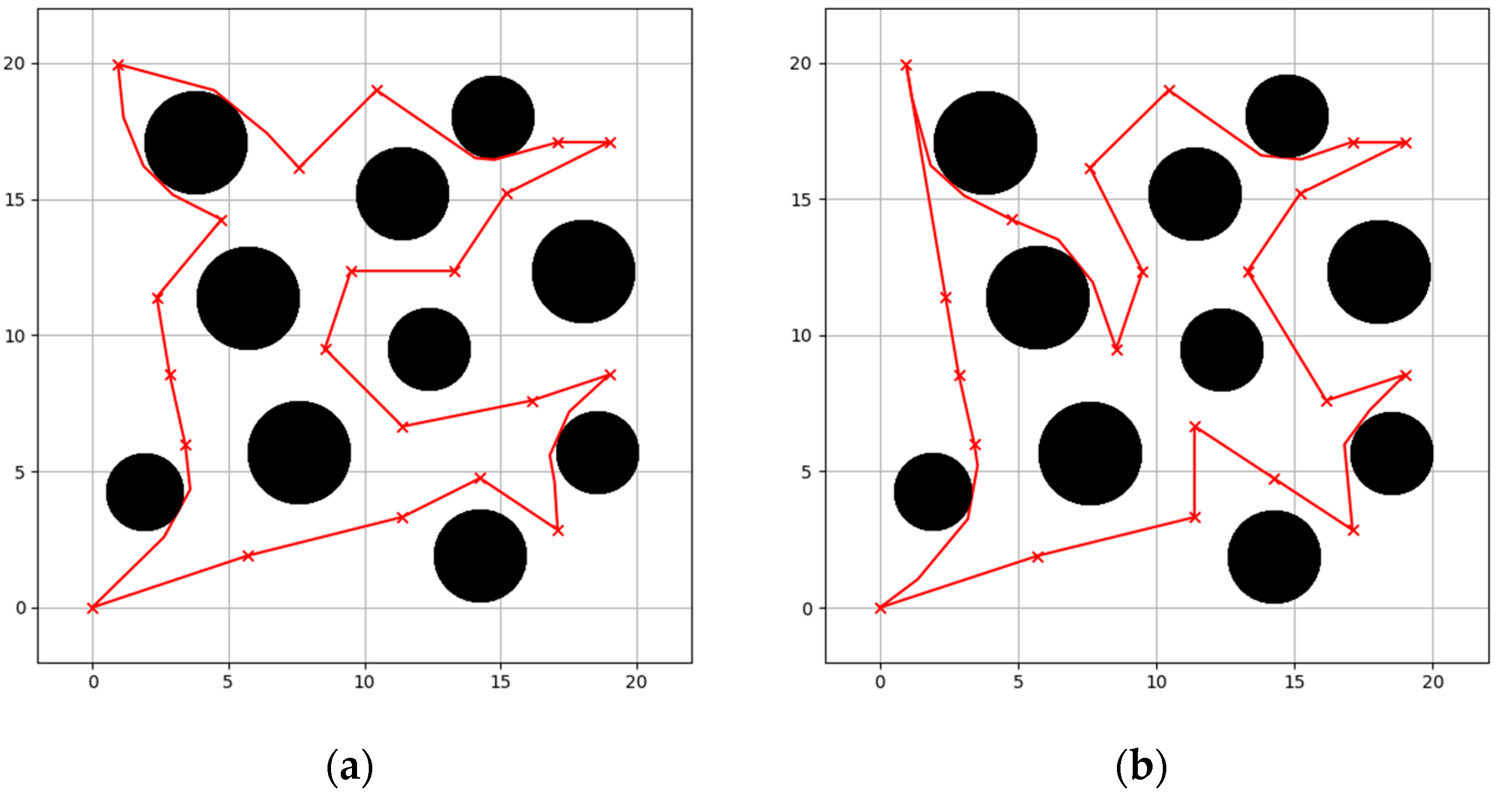
Based on the traversal order obtained in Section 4.2, the Informed-RRT* algorithm is employed to plan the optimal global path from the starting point, through all the target points in order and back to the starting point. If the direct line segment between two adjacent target points in the traversal order does not intersect with any obstacle circles, that line segment can be used directly as the path between these two points, with the path cost equal to the length of the line segment. Experiments show that this method can further reduce the total path cost and improve the speed of global planning. The global paths planned for the four traversal orders in both task scenarios are shown in Figure 11.

4.4. Simulation Experiment Analysis

To avoid the cumulative interference brought about by the uncertainty of the Informed-RRT* algorithm, 10 global planning instances are conducted for each of the four traversal orders in the two scenarios. The average of the planning results is shown in Table 3.
Table 3 shows that the total path costs of the plans according to order 1 and 3 in the two task scenarios are reduced by 4.1663% and 4.0272%, respectively, compared to the orders 2 and 4. This result thoroughly tests the excellence of the solution obtained by entering the estimated path cost matrix into the TSP.
The time cost of each stage of the algorithm under three cost matrix inputs is recorded, as shown in Table 4.
The main difference in the time costs of the three groups of experiments is reflected in the construction of the cost matrix. At this point, the construction of the actual path cost matrix cannot avoid times of actual planning, which takes far longer than constructing the other two types of cost matrices. With the expansion of the task scenario and the increase in target points, the number of plannings grows quadratically, and the time cost of constructing the actual path cost matrix will also increase dramatically. Conversely, the calculation amount for constructing the Euclidean distance cost matrix is small, and the time cost is negligible. However, it does not fully reflect the real cost of the path between two points and cannot provide a reliable basis for solving the TSP for the traversal order. The construction of the estimated path cost matrix takes extremely little time, yet it can use the estimated path cost between two points that fits the actual planning result as the basis for solving the TSP, which enhances the rationality of the obtained traversal order.

5. Prototype Experiment Design and Analysis

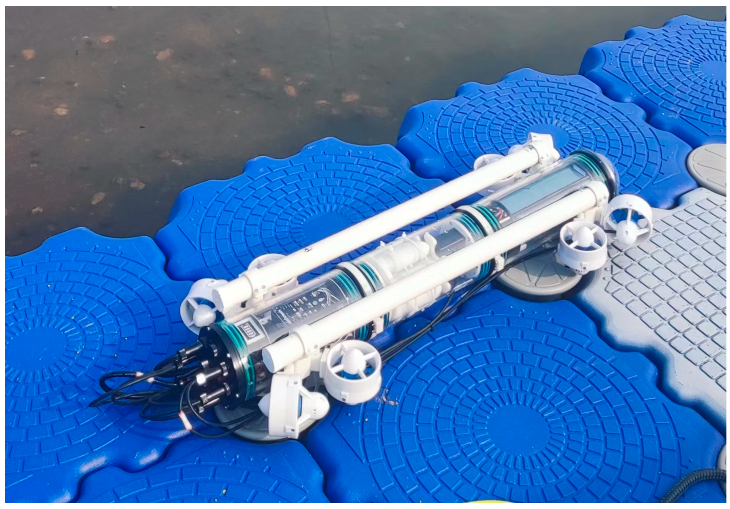
The UUV prototype designed according to the needs of the verification experiment is shown in Figure 12.
The UUV has eight thrusters, which can realize closed-loop control of four degrees of freedom movement, including rising and sinking, moving forward and backward, moving left/right, and turning in place. The device is structured in three sections, consisting of a battery compartment, payload compartment, and control compartment. The control compartment integrates the flight control system and payload control system and is connected to a communication buoy by a buoyancy line. The relevant technical parameters are shown in Table 5.
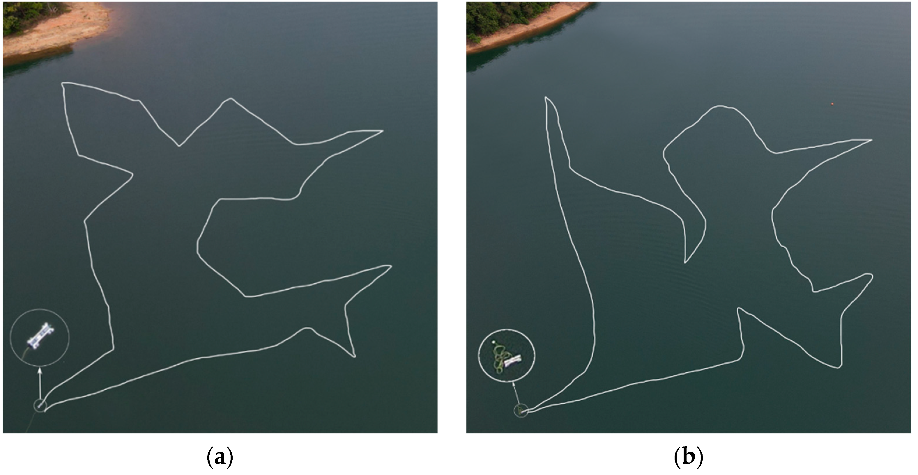
Two open water areas with an area of 100 m × 100 m in a certain lake were selected as the experiment sites. Through ground station software, electronic fences and target point coordinates are set in the experimental waters according to task scenario A. In the drone filming experiment, to facilitate the statistics of the sailing distance and time, the UUV does not conduct payload operation experiments after reaching each target point. The UUV is deployed from the starting point, sails at a constant depth close to the water surface, and returns to the starting point after passing through all the target points in order. Under the two traversal orders, the aerial view of the unmanned aerial vehicle is shown in Figure 13.
Ground station software data show that the total distances covered by the UUV under the two orders are 494 m and 518 m, respectively, and the sailing times are 605 s and 644 s, respectively. The total distance and time of the global path planned according to order 1 are shorter, which further verifies the effectiveness of the algorithm results.

6. Conclusions and Prospects

In response to the deficiencies in existing methodologies for multi-target path planning, this study put forth an innovative neural network-based strategy for path cost estimation. This pioneering approach not only augments precision but also significantly boosts computational efficiency in anti-mine operations involving UUVs. Our research’s novelty rests in transmuting the intricate multi-target path planning problem into a more manageable TSP. This paradigm shift streamlines the planning process without compromising its effectiveness. Central to our approach is the deployment of a neural network trained for path cost estimation. This network efficiently generates accurate cost matrices, thereby depicting the shortest possible path between any two target points, considering potential obstacles. In contrast to conventional strategies, our method dispenses with redundant planning periods and addresses the reliability conundrum associated with Euclidean distance cost matrices. Furthermore, our design of the objective function thoughtfully considers crucial factors such as path cost and operational time, thus enhancing the algorithm’s speed and reliability. Concrete evidence supporting the utility and effectiveness of our algorithm is presented through rigorous trials using an actual UUV prototype in a lake setting.
In the forthcoming research, our attention will be devoted to broadening the current methodology’s reach to incorporate a three-dimensional environment. Within this framework, pinpointing apt representation parameters and cultivating a corresponding estimation network will emerge as crucial research directives. By undertaking these initiatives, we anticipate opening pathways for a more resilient and adaptable approach to multi-target path planning. Such evolution could profoundly augment the efficiency and effectiveness of anti-mine operations employing UUVs, heralding a significant breakthrough in the field.

Author Contributions

Conceptualization, S.Z. and Z.W.; methodology, S.Z.; software, S.Z. and L.L.; validation, S.Z., Z.W. and L.L.; formal analysis, H.L.; investigation, H.L.; resources, L.L.; data curation, L.L.; writing—original draft preparation, S.Z.; writing—review and editing, S.Z.; visualization, Z.W.; supervision, H.L.; project administration, Z.W.; funding acquisition, H.L. All authors have read and agreed to the published version of the manuscript.

Funding

This research was funded by the National Natural Science Foundation of China, grant number 42122025.

Institutional Review Board Statement

Not applicable.

Informed Consent Statement

Not applicable.

Data Availability Statement

Not applicable.

Conflicts of Interest

The authors declare no conflict of interest.

References

  1. Galceran, E.; Palomeras, N.; Carreras, M. Profile Following for Inspection of Underwater Structures. Paladyn J. Behav. Robot. 2013, 4, 209–220. [Google Scholar] [CrossRef] [Green Version]
  2. Manaranche, M. France Plots Route to New Unmanned MCM Capability. Warsh. Technol. 2011, 37–38. [Google Scholar]
  3. Daoliang, L.; Peng, W.; Ling, D. Path Planning Technologies for Autonomous Underwater Vehicles-A Review. IEEE Access 2018, 7, 9745–9768. [Google Scholar] [CrossRef]
  4. Lin, W.; Delgado, J.G.; Gause, D.C.; Vassiliadis, S. Hybrid Newton-raphson Genetic Algorithm for the Traveling Salesman Problem. Cybern. Syst. 1995, 26, 387–412. [Google Scholar] [CrossRef]
  5. Rubio-Sierra, C.; Domínguez, D.; Gonzalo, J.; Escapa, A. Path Planner for Autonomous Exploration of Underground Mines by Aerial Vehicles. Sensors 2020, 20, 4259. [Google Scholar] [CrossRef] [PubMed]
  6. Venkatesh, P.; Singh, A. An Artificial Bee Colony Algorithm with Variable Degree of Perturbation for the Generalized Covering Traveling Salesman Problem. Appl. Soft Comput. 2019, 78, 481–495. [Google Scholar]
  7. Minghao, L.; Lijun, Q.; Jianfeng, J. A Multigoal Path-Planning Approach for Explosive Ordnance Disposal Robots Based on Bidirectional Dynamic Weighted-A* and Learn Memory-Swap Sequence PSO Algorithm. Symmetry 2023, 15, 1052. [Google Scholar] [CrossRef]
  8. Daichuan, Y.; Chenglin, W. Multiple Targets Robot Path Planning Based on Ant Colony and Improved Probabilistic Road Map. J. Hangzhou Dianzi Univ. (Nat. Sci.) 2017, 37, 63–67. [Google Scholar] [CrossRef]
  9. Wenjun, Y.; Kuixiang, X.; Zhejing, B. A 3D Space Multi-Target Path Planning Method Combining RRT and Ant Colony Optimization Algorithms. Patent No. CN109211242B,2020-10-23, 23 October 2020. [Google Scholar]
  10. Yu, J.-b.; Chen, Z.-h.; Deng, W.; Xu, J.-p.; Zhao, Z.-y.; Wang, X.-y. A Traversal Multi-target Path Planning Algorithm for Unmanned Cruise Ship. Comput. Eng. Sci. 2023, 45, 840–848. [Google Scholar] [CrossRef]
  11. Xu, R.; Cao, M.; Huang, M.; Zhu, Y.H. Research on the Quasi-TSP problem based on the improved grey wolf optimization algorithm: A case study of tourism. Geogr. Geo-Inf. Sci. 2018, 34, 14–21. (In Chinese) [Google Scholar]
  12. Wu, X.; Gao, Z.; Yuan, S.; Hu, Q.; Dang, Z. A Dynamic Task Allocation Algorithm for Heterogeneous UUV Swarms. Sensors 2022, 22, 2122. [Google Scholar] [CrossRef] [PubMed]
  13. Mahmoudzadeh, S.; Powers, D.; Atyabi, A. UUV’s Hierarchical DE-Based Motion Planning in a Semi Dynamic Underwater Wireless Sensor Network. IEEE Trans. Cybern. 2019, 49, 2992–3005. [Google Scholar] [CrossRef] [PubMed]
  14. Gammell, J.D.; Srinivasa, S.S.; Barfoot, T.D. Informed RRT*: Optimal Sampling-based Path Planning Focused via Direct Sampling of an Admissible Ellipsoidal Heuristic. In Proceedings of the 2014 IEEE/RSJ International Conference on Intelligent Robots and Systems, Chicago, IL, USA, 14–18 September 2014; pp. 2997–3004. [Google Scholar] [CrossRef] [Green Version]
  15. Mashayekhi, R.; Idris, M.Y.I.; Anisi, M.H.; Ahmedy, I.; Ali, I. Informed RRT*-Connect: An Asymptotically Optimal Single-Query Path Planning Method. IEEE Access 2020, 8, 19842–19852. [Google Scholar] [CrossRef]
  16. Tao, G.; Michalewicz, Z. Evolutionary Algorithms for the TSP. In Proceedings of the 5th International Conference on Parallel Problem Solving from Nature, Amsterdam, The Netherlands, 27–30 September 1998; Springer: Berlin/Heidelberg, Germany, 2003; pp. 803–812. [Google Scholar]
  17. Kesheng, C.; Sidong, X.; Peng, G. Adaptive Temperature Rising Simulated Annealing Algorithm for Traveling Salesman Problem. Control. Theory Appl. 2021, 38, 245–254. [Google Scholar] [CrossRef]
  18. Silva, C.; Aguiar, A.; Lima, P.; Dutra, I. Mapping a logical representation of TSP to quantum annealing. Quantum Inf. Process. 2021, 20, 386. [Google Scholar] [CrossRef]
  19. Qing, H.; Yile, W.; Tongwei, X. Application of improved genetic simulated annealing algorithm in TSP optimization. Control. Decis. 2018, 33, 219–225. [Google Scholar] [CrossRef]
  20. Da, C.; Xiaoming, Y.; Sheng, L. Ant Colony Algorithm with n-α-Measure and Migration Learning. Arab. J. Sci. Eng. 2023, 48, 1873–1890. [Google Scholar] [CrossRef]
  21. Tuani, A.F.; Keedwell, E.; Collett, M. Heterogenous Adaptive Ant Colony Optimization with 3-opt local search for the Travelling Salesman Problem. Appl. Soft Comput. 2020, 97, 106720. [Google Scholar] [CrossRef]
  22. Hehua, L.; Chao, C.; Jing, C. An Improved Genetic Algorithm for Solving Travel Salesman Problem. Trans. Beijing Inst. Technol. 2013, 33, 390–393. [Google Scholar] [CrossRef]
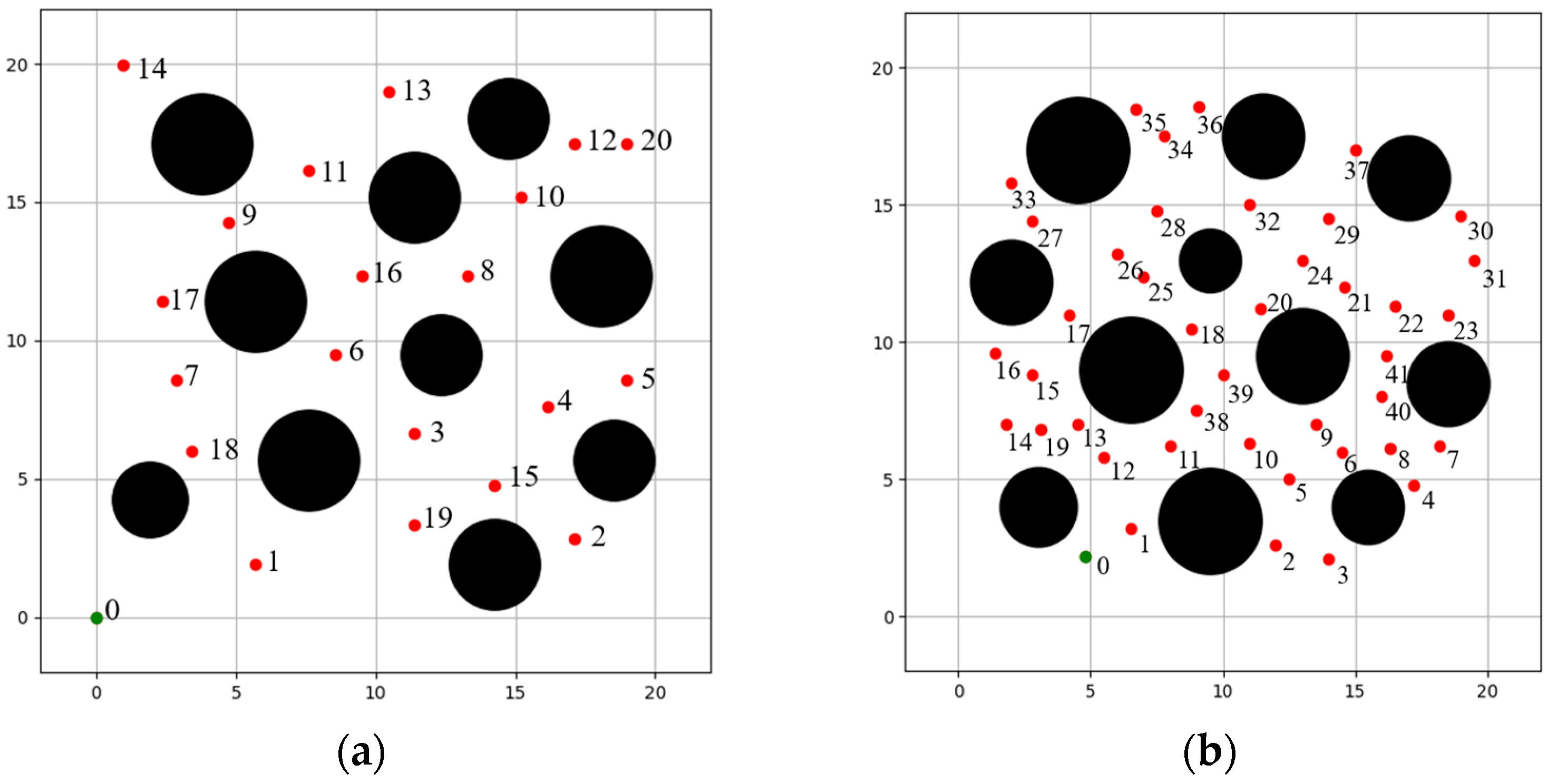
Figure 1. Feature map of the task scenario (a) Scenario A; (b) Scenario B.
Jmse 11 01582 g001
Figure 2. Schematic diagram of UUV navigation operations.
Jmse 11 01582 g002
Figure 3. The overall framework of multi-target path planning algorithm.
Jmse 11 01582 g003
Figure 4. Flowchart of the Informed-RRT* algorithm.
Jmse 11 01582 g004
Figure 5. Schematic diagram of dataset creation (a) General planning scenario; (b) Scenario after coordinate transformation.
Jmse 11 01582 g005
Figure 6. Schematic diagram for calculating the characterization parameters of single obstacle circle.
Jmse 11 01582 g006
Figure 7. Schematic diagram for calculating the characterization parameters of double obstacle circle.
Jmse 11 01582 g007
Figure 8. Flowchart of genetic algorithm solving the TSP.
Jmse 11 01582 g008
Figure 9. Comparison of 100 planning results with estimation results.
Jmse 11 01582 g009
Figure 10. Iteration process of genetic algorithm (a) scenario A; (b) scenario B.
Jmse 11 01582 g010
Figure 11. Global path planning results (a) Order 1 in scenario A; (b) Order 2 in scenario A; (c) Order 3 in scenario B; (d) Order 4 in scenario B.
Jmse 11 01582 g011aJmse 11 01582 g011b
Figure 12. Prototype of UUV.
Jmse 11 01582 g012
Figure 13. Water surface navigation test of UUV (a) Aerial view of order 1 in scenario A; (b) Aerial view of order 2 in scenario A.
Jmse 11 01582 g013
Table 1. Error analysis of path cost planning and estimation in various situations.
GroupEstimated Cost ValueMean Absolute ErrorRoot Mean Square ErrorUp/Down Distribution
Situation 16.021890.041210.0650541/59
Situation 210.008910.059340.0739739/61
Situation 313.841250.016040.0285455/45
Situation 417.520380.069160.0978850/50
Situation 521.359930.079080.1027836/64
Table 2. Genetic algorithm parameter settings.
ParameterScenario AScenario B
Population Size80100
Number of Iterations200600
Mutation Probability0.0050.008
Crossover Probability0.80.9
Number of Traversal Points2142
Table 3. Comparison of path costs of three cost matrix algorithms.
Task ScenariosInput MatrixOrder
Number
10 Global Planning Average Path Cost
A D r e 196.6899
D e s
D e d 2100.8934
B D r e 3103.3183
D e s
D e d 4107.6537
Table 4. Comparison of time costs under three cost matrix inputs.
Task ScenariosInput MatrixTime Cost to Construct Cost MatrixTime Cost to Solve TSPAverage Time Cost of 10 PlanningsTotal Time Cost
A D r e 1296.62340.84458.41831305.8862
D e s 0.25220.81379.4842
D e d 0.00000.82067.30578.1263
B D r e 5326.21644.26745.22645335.7102
D e s 0.93914.289810.4553
D e d 0.00004.19479.565013.7597
Table 5. Parameters of the UUV.
ParameterSpecific Parameter
Size900 × 350 × 180 (millimeters)
Endurance1.5 (hours)
Maximum Speed3 (knots)
Maximum Diving Depth10.0 (meters)
Positioning Accuracy<1.5 (meters)
Disclaimer/Publisher’s Note: The statements, opinions and data contained in all publications are solely those of the individual author(s) and contributor(s) and not of MDPI and/or the editor(s). MDPI and/or the editor(s) disclaim responsibility for any injury to people or property resulting from any ideas, methods, instructions or products referred to in the content.