Article

Quality Assessment of Sea Surface Salinity from Multiple Ocean Reanalysis Products

1
College of Meteorology and Oceanography, National University of Defense Technology, Changsha 410073, China
2
School of Systems Engineering, National University of Defense Technology, Changsha 410073, China
3
School of Economics and Management, Nanjing University of Technology, Nanjing 210000, China
*
Author to whom correspondence should be addressed.
J. Mar. Sci. Eng. 2023, 11(1), 54; https://doi.org/10.3390/jmse11010054
Submission received: 11 October 2022 / Revised: 13 December 2022 / Accepted: 20 December 2022 / Published: 30 December 2022
(This article belongs to the Section Physical Oceanography)

Abstract

:
Sea surface salinity (SSS) is one of the Essential Climate Variables (ECVs) as defined by the Global Climate Observing System (GCOS). Acquiring high-quality SSS datasets with high spatial-temporal resolution is crucial for research on the hydrological cycle and the earth climate. This study assessed the quality of SSS data provided by five high-resolution ocean reanalysis products, including the Hybrid Coordinate Ocean Model (HYCOM) 1/12° global reanalysis, the Copernicus Global 1/12° Oceanic and Sea Ice GLORYS12 Reanalysis, the Simple Ocean Data Assimilation (SODA) reanalysis, the ECMWF Oceanic Reanalysis System 5 (ORAS5) product and the Estimating the Circulation and Climate of the Ocean Phase II (ECCO2) reanalysis. Regional comparison in the Mediterranean Sea shows that reanalysis largely depicts the accurate spatial SSS structure away from river mouths and coastal areas but slightly underestimates the mean SSS values. Better SSS reanalysis performance is found in the Levantine Sea while larger SSS uncertainties are found in the Adriatic Sea and the Aegean Sea. The global comparison with CMEMS level-4 (L4) SSS shows generally consistent large-scale structures. The mean ΔSSS between monthly gridded reanalysis data and in situ analyzed data is −0.1 PSU in the open seas between 40° S and 40° N with the mean Root Mean Square Deviation (RMSD) generally smaller than 0.3 PSU and the majority of correlation coefficients higher than 0.5. A comparison with collocated buoy salinity shows that reanalysis products well capture the SSS variations at the locations of tropical moored buoy arrays at weekly scale. Among all of the five products, the data quality of HYCOM reanalysis SSS is highest in marginal sea, GLORYS12 has the best performance in the global ocean especially in tropical regions. Comparatively, ECCO2 has the overall worst performance to reproduce SSS states and variations by showing the largest discrepancies with CMEMS L4 SSS.

1. Introduction

Salinity, as an Essential Climate Variable (ECV), significantly affects the hydrological cycle, ocean circulation, and earth climate. As a passive tracer in the ocean, the spatial distribution of Sea Surface Salinity (SSS) shows highly consistent patterns with the evaporation-minus-precipitation (E-P) field in most areas of the global ocean. The structure and evolution of SSS depict how the freshwater input from precipitation, river runoff, ice melting, etc. are redistributed throughout the ocean, and how such sea surface signals will propagate downward and then affect the full volume of seawater through diffusive and advective processes [1]. For this reason, salinity has been widely used as an indicator of the intensifying hydrological cycle under global warming [2,3]. As a key participant in ocean dynamics, salinity also contributes to the horizontal pressure gradients and vertical stability by changing the seawater density along with temperature, which further affects the evolution of thermohaline circulation [4] and mixing processes [5]. These changes are closely linked to the air-sea fluxes and are ultimately associated with the earth climate [6].
The global salinity maps are mainly obtained from satellite retrievals, in situ measurements, and ocean reanalysis. Among them, ocean reanalysis products are superior to objectively analyzed products in providing increased spatiotemporal resolution and a multi-variate dynamical consistency [7,8,9]. However, they still suffer from low accuracy compared with that of directly observed data, which is especially true in coastal areas [10], marginal seas [11] and polar regions [12,13], where the currently available salinity observations are not sufficient to constrain the dynamical model. Over the last decade, the performance of ocean reanalysis has significantly improved thanks to increased model resolution [14], better physics [15], better atmospheric forcing data [16], more abundant observation input [17] and, advanced assimilation schemes [18]. This is evidenced by assessment studies showing higher verification skill scores in successive versions of reanalysis products.
Recent studies suggest that the assimilation of observed salinity help improve the overall quality of ocean reanalysis by providing more accurate initial state estimates for the dynamical models as the imbalance between temperature and salinity is effectively reduced, which ultimately results in the improvement of El Niño Southern Oscillation (ENSO) prediction skills [19]. To date, many institutions have developed ocean reanalysis systems (ORAs) to build up historical ocean data products and provide initial conditions for ocean forecast system, which provides long-term historical salinity data at high spatial and temporal resolutions. Due to the scarcity of in situ salinity observations, earlier versions of reanalysis products generally assimilate observed temperature data, whereas the assimilation of observed salinity is either absent or directly constructed from a local temperature-salinity (T–S) relationship [20]. After the launch of the International Argo Project, the real-time temperature and salinity profiles in the upper ocean have been collected and achieved global coverage from 2006 onwards. As a result, most ocean reanalysis products after 2006 have assimilated both temperature and salinity profiles.
Quality assessment of SSS reanalysis has not been frequently seen in recent studies. Instead, only those focusing on the salinity profiles simulated by several individual reanalysis systems have been widely conducted. For example, the author of [21] assessed the quality of upper salinity content above 1500 m reproduced by ten reanalysis systems. The author of [10] indicates that data assimilation has effectively improves the fit of ORAS5 to the in situ salinity measurements. The long-term variations of salinity anomalies as reproduced by multiple regional reanalysis products have been comprehensively assessed by several recent studies [22,23,24]. Moreover, most previous validation efforts, no matter the global or regional scale, have generally focused on single or limited numbers of reanalysis products. The Ocean Reanalysis Intercomparison project (ORA-IP) initiated in 2011 helped to proceed the intercomparison and validation of in salinity from an ensemble of existing global ocean reanalysis [25,26]. However, some eddy-resolving reanalysis products, such as the 1/12° HYCOM and GLORYS12 products, are not in the scope of the above studies but are still worthy of a comprehensive assessment due to their capacity to resolve mesoscale ocean structures. Moreover, previous evaluation studies have generally focused on the mean state and variations of SSS at single spatial or temporal scale, since the emphasis is mainly placed on the quality of temperature and ocean current data.
This paper is organized into four sections. Data and comparing methods are summarized in Section 2. The results of comparison against objectively analyzed datasets in a typical marginal sea, in the global ocean and in the tropical areas are described in Section 3. The conclusions and discussions are presented in Section 4.

2. Materials and Methods

2.1. Ocean Reanalysis

Five state-of-the-art ocean reanalysis products with high resolution, long time span and global coverage are included in this study, including the Hybrid Coordinate Ocean Model (HYCOM) 1/12° global reanalysis, the Copernicus Global 1/12° Oceanic and Sea Ice GLORYS12 Reanalysis, the Simple Ocean Data Assimilation (SODA) reanalysis, the ECMWF Oceanic Reanalysis System 5 (ORAS5) product and the Estimating the Circulation and Climate of the Ocean Phase II (ECCO2) reanalysis. Critical information of the above 5 products is summarized in Table 1.
HYCOM is an eddy-resolving Ocean General Circulation Model (OGCM) with primitive equations Boussinesq approximation, which can be used for a diverse range of investigations from coastal to open sea circulation [27]. Among multiple HYCOM ocean products, the outputs of Global Ocean Forecast System 3.0 (GOFS 3.0) are utilized in this study. The GOFS 3.0 GLBu Reanalysis product from 1993 to 2013 is selected and temporal coverage is extended to November 2018 by including the GOFS 3.0 GLBu Analysis product. The HYCOM Reanalysis/Analysis product has 1/12° spatial resolution, which is capable of resolving mesoscale ocean structures. The measurements from altimeters, XBTs, Argo, and other buoys are assimilated into the HYCOM model via the Navy Coupled Ocean Data Assimilation (NCODA) system on a daily basis. More descriptions of these products are available from https://www.hycom.org/dataserver/gofs-3pt1/analysis (accessed on 14 June 2021).
GLORYS12 is another eddy-resolving ocean and sea ice reanalysis implemented in the CMEMS framework [28,29]. The GLORYS12V1 Reanalysis product is interpolated from GLORYS2V4, which is the output of the Nucleus for European Modeling of the Ocean (NEMO) model after assimilating the Sea Surface Height (SSH) data from multiple satellites and T/S profiles collected by various platforms. The reduced-order Kalman filter is used for data assimilation, while the three-dimensional variational (3D-VAR) assimilation scheme is additionally applied to correct the slowly-evolving large-scale errors [28]. The NEMO model is initialized by EN 4.2.0 monthly gridded climatology and driven by the European Centre for Medium-Range Weather Forecasts (ECMWF) ERA-Interim atmospheric reanalysis. The time range of GLORYS12V1 Reanalysis is from October 1992 to December 2019 with a spatial resolution of 1/12°.
The SODA3 reanalysis system is primarily based on the Modular Ocean Model version 5 (MOM5) with a horizontal resolution of 0.25° × 0.25° and 50 uneven vertical layers [30]. Among the multiple versions of SODA3 reanalysis, the SODA 3.11.2 product is assessed in this study. The hydrographic input of SODA3 from the World Ocean Database 13 (WOD13) is assimilated by using the least squares fit algorithm, the data volume of which has increaby sed 40% compared with the WOD09 assimilated by SODA2. Additionally, SODA3 ingested an upgraded version of in situ SST product (ICOADS version 5 release 2 SST) [31]. Note that SODA3 does not assimilate sea level and ocean current observations.
ORAS5 is a global ocean and sea-ice ensemble reanalysis product for the ECMWF OCEAN5 system in its behind-real-time stream, which provides historical ocean and sea-ice conditions from 1979 to present [14]. ORAS5 used NEMO 3.4.1 model with a tripolar grid allowing eddies to be simulated approximately between 50° S and 50° N. The horizontal resolution is ~25 km in tropical ocean and increases to 9 km towards the polar regions. The atmospheric forcing field for the NEMO model in ORAS5 is derived from the ERA-Interim reanalysis product. Data assimilation is conducted with NEMOVAR in its 3D-Var First Gauss at Appropriate Time (FGAT) configuration to assimilate T/S profiles from EN4, XBT and MBT, SST and sea ice from HadISST2 and OSTIA operational product, as well as sea-level anomalies (SLAs) from AVISO DT2014 [32].
ECCO2 data syntheses are derived from a global full-depth-ocean and sea-ice configuration of the Massachusetts Institute of Technology general circulation model (MITgcm) by a least squares fit method to the available satellite and in situ observational data. ECCO2 employs a cube-sphere grid projection that permits relatively even grid spacing throughout the ocean and avoids singularities in polar regions. ECCO2 has 50 vertical levels ranging from 10 m near the sea surface to approximately 450 m at the bottom 6150 m. The data assimilation is achieved by using a Green’s function approach to constrain limited variables, including SLA from altimeter data, sea surface temperature from GHRSST-PP, temperature and salinity profiles from WOCE, TAO, ARGO, XBT and other platforms.

2.2. In Situ Analyzed Product

As a reference for validation, the CMEMS Level-4 (L4) SSS product is utilized which provides global gap-free L4 analyzed maps of SSS and Sea Surface Density (SSD). This product is developed by the National Research Council (CNR) production unit and distributed by the CMEMS platform (Product ID: MULTIOBS_GLO_PHY_S_SURFACE_MYNRT_015_013). The SSS and SSD fields are generated through a MultiVariate Optimal Interpolation (MVOI) algorithm that combines both the Soil Moisture and Ocean Salinity (SMOS) satellite SSS and in situ salinity measurements with satellite SST. The CMEMS L4 SSS product has been similarly used as a reference for the validation of L4 SSS products in the Mediterranean Sea, where improving the quality of SSS data is challenging due to the scarcity of in situ measurements. Therefore, we use the CMEMS L4 product for validation both in the global ocean and within the marginal sea.

2.3. Mooring Buoy

Long-term salinity records from the Global Tropical Moored Buoy Array (GTMBA) are introduced as ground truth for assessment in tropical ocean. Each buoy provides continuous salinity observation data near the sea surface (~1 m) with a high temporal resolution in the entire reanalysis period we selected for this study. The GTMBA consists of Tropical Atmosphere Ocean (TAO) data in the Pacific [33], the Pilot Research Moored Array in the Tropical Atlantic (PIRATA) [34] and the Research Moored Array for African-Asian Australian Monsoon Analysis and Prediction (RAMA) in the Indian Ocean [35]. They record temperature and salinity every 10 min, and the raw data have been postprocessed into hourly data with the accuracy of 0.2 PSU [36]. To compare with reanalysis SSS, only surface salinity measurements at 1 m with high QC flag are taken into account. A 7-day moving average is applied to the postprocessed hourly time series for a consistent temporal resolution with the collocated reanalysis data.

2.4. Assessment Strategy

The assessment of SSS reanalysis in this study is primarily based on the calculation of fundamental statistic parameters, including the ΔSSS (SSSreanalysis − SSSin situ), the standard deviation, the Root Mean Square Deviation (RMSD), and the Pearson correlation coefficient, together with p-value. The corresponding algorithm for each parameter is listed in Table 2.
The strategy of assessment is described as follows. First, the performance of SSS reanalysis within subpolar marginal seas is evaluated by a comparison against CMEMS L4 SSS in the Mediterranean Sea. The regional assessment is primarily based on the estimations of error structure in each SSS reanalysis by calculating the mean SSS values, standard deviation, ΔSSS and RMSD consistently on a 0.25° grid. After that, taking CMEMS L4 SSS as reference, a global comparison is conducted by illustrating the spatial distribution of ΔSSS, RMSD and correlation coefficient from 60° N to 60° S excluding polar regions. We also analyze the mean ΔSSS and RMSD values at four different spatial resolutions, 0.25°, 1° and 3° and 10°. Finally, the quality of weekly SSS variations in the tropical ocean as reproduced by five SSS reanalysis products are validated against the long-term SSS records provided by GTMBA.

3. Results

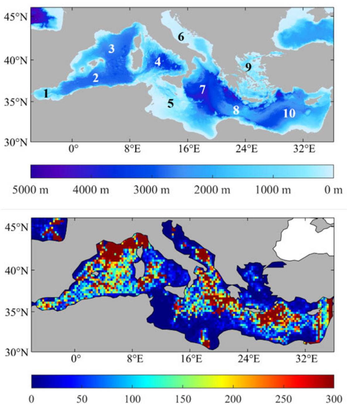
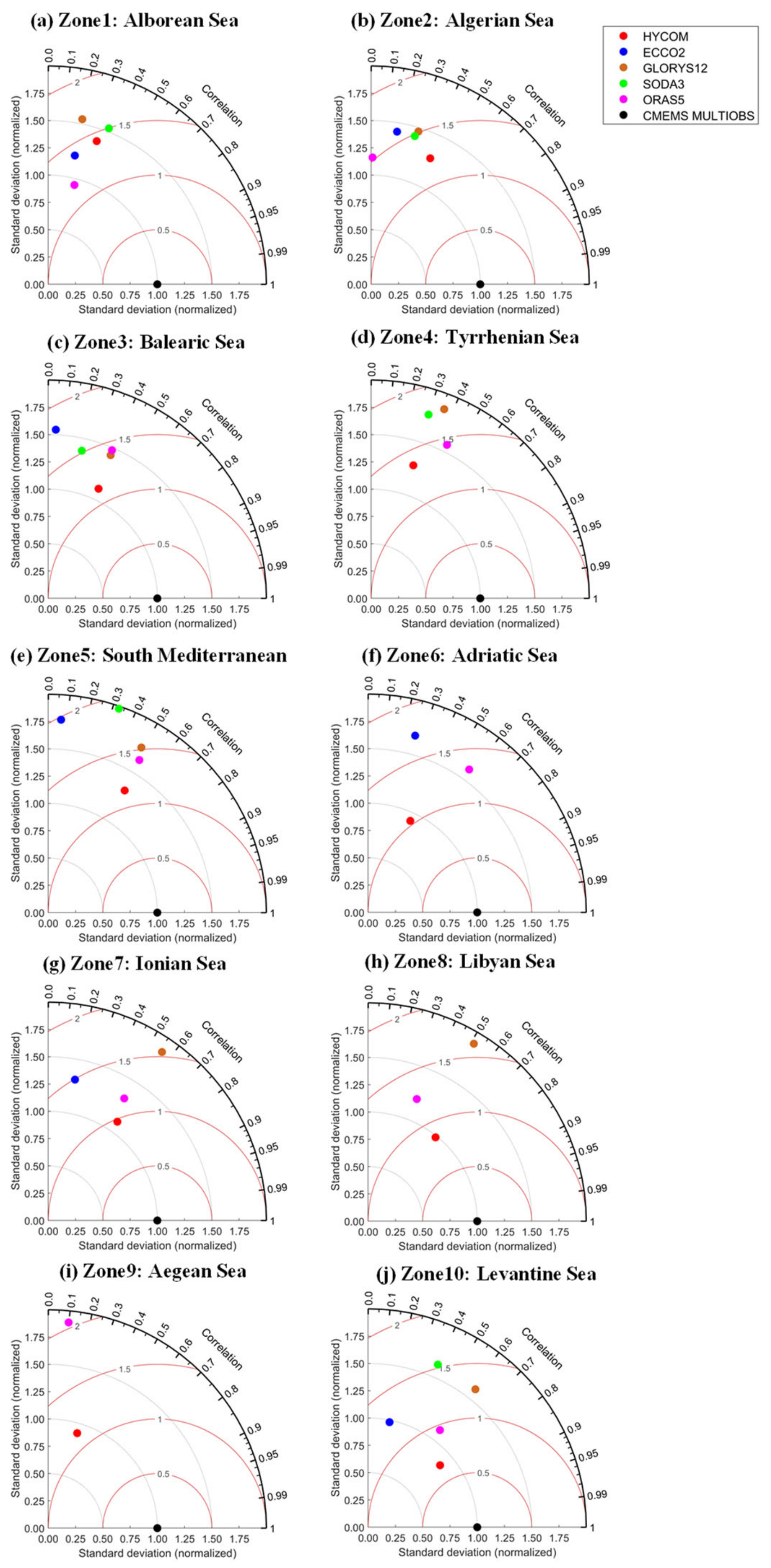
3.1. Regional Assessment in the Mediterranean Sea

Differing from other open sea regions, the Mediterranean Sea is characterized by very high salinity because water balance over this basin is fundamentally characterized by an excess of evaporation over precipitation and river runoff. High-resolution ocean reanalysis contributes to a better understanding of the SSS dynamics in this marginal sea, but unfortunately, the SSS reanalysis performance is significantly limited by the sparsity of in situ salinity measurement data that are available to be used for both data assimilation and objective interpolations. The quality of satellite SSS in the Mediterranean Sea also suffers from errors caused by Radio Frequency Interference (RFI) and land contaminations, which are not as valuable for data assimilation as in situ SSS measurements. Therefore, a regional assessment of reanalysis SSS in the Mediterranean Sea is necessary to examine whether ocean reanalysis has the capacity to reproduce SSS dynamics in a marginal sea and which of the various SSS reanalysis products are more suitable for scientific applications in a typical marginal sea. Figure 1 shows the spatial distribution of in situ SSS measurements in the Mediterranean Sea provided by various platforms that has been merged by CMEMS L4 product. The in situ SSS measurements cover more than 70% areas of the Mediterranean Sea except for some coastal areas. This deficiency can be partly mitigated by merging satellite SSS. Therefore, CMEMS L4 SSS is suitable to serve as reference in this marginal sea which combines the CORA reanalysis and SMOS CATDS product to obtain a better SSS state estimation over this basin.
Figure 2 and Figure 3 show the spatial distribution of mean SSS and STD values in the Mediterranean Sea as obtained from five reanalysis products and CMEMS L4 SSS from January 2005 to December 2016, respectively. Their large-scale SSS patterns show generally consistent structures between ocean reanalysis and in situ analyzed products, such as the relatively fresher water in the Alboran Sea, the high salinity water in the Levantine Sea and the obvious SSS front in the Adriatic Sea and Aegean Sea. The SSS values ranges from 35.5 in the Alboran Sea to 40 PSU in the Western Mediterranean with a smooth positive gradient extending in the zonal direction. The ORAS5 product shows the highest mean SSS value (36.7 PSU) compared with CMEMS L4 SSS (35.8 PSU), HYCOM (35.9 PSU), GLORYS12 (35.6 PSU), ECCO2 (34.7 PSU) and SODA3 (35.1 PSU) data. Similarly, the STD patterns also present significant discrepancies among six products. All five reanalysis products tend to overestimate the SSS variances with the highest mean STD value of 0.45 PSU from SODA 3.11.2 compared with that of HYCOM (0.23 PSU), ECCO2 (0.28 PSU), ORAS5 (0.29 PSU) and GLORYS12 (0.42 PSU), which is more than twice as large as that of CMEMS L4 SSS (0.19 PSU). The above suggests that HYCOM reanalysis has best performance in reproducing the mean SSS state and its variations in the Mediterranean Sea.
To further verify the above statistics, Figure 4 shows the corresponding spatial distribution of ΔSSS and Correlation Coefficient (CC) of five reanalysis products against CMEMS L4 in situ analyzed SSS. The small ΔSSS values are generally collocated with high CC values, which are widely distributed in the eastern part of the Mediterranean Sea than the western part, possibly due to the less influence from Atlantic water masses away from. Large ΔSSS and low CC values are mainly distributed near the coast and in the gulfs, such as in the north part of the Balearic Sea, in the Northern end of the Adriatic Sea and Aegean Sea. The overall negative ΔSSS values are synchronously seen from each reanalysis product with the smallest ΔSSS (0.07 PSU) and highest mean CC (0.47) belonging to the HYCOM reanalysis product. Comparatively, the ECCO2 and SODA3 products contains significantly larger negative biases especially in the Ionian Sea, the Libyan Sea and the Aegean Sea where several ΔSSS values reach as large as -1 PSU. It is noted that ECCO2 has very large ΔSSS values and very low CC values among the five-model reanalysis, which corresponds to the significantly lower mean SSS in Figure 2 and anomalous large STD values in the middle part of the Mediterranean Sea. Although the GLORYS12 product well reproduces the mean SSS values across the basin, it presents too large SSS variances compared with CMEMS L4 SSS data.
Ten subregions in the Mediterranean Sea are divided to evaluate the SSS reanalysis performance in different ocean conditions, including the Alboran Sea, the Algerian Sea, the Balearic Sea, the Tyrrhenian Sea, the Southern Mediterranean, the Adriatic Sea, the Ionian Sea, the Libyan Sea, the Aegean Sea and the Levantine Sea. (Figure 1, upper panel). Statistics for each region are quantified separately in the Taylor diagrams of Figure 5. The Taylor diagram is a statistical tool to evaluate the simulation capacity of multiple numerical models [37]. It combines the correlation coefficient, the standard deviation and RMSD in the same semicircle diagram in order to visualize the overall data quality by distance in plane space. Generally, the performance of SSS reanalysis is not optimistic in the majority of subregions in the Mediterranean Sea, with most CC values smaller than 0.5, normalized RMSD values larger than 1 and normalized STD values larger than 1, respectively. The performance of HYCOM is generally better than other four reanalysis products in most subregions except for the Alboran Sea where ORAS5 shows higher CC and lower normalized RMSD. Statistics from the Taylor diagrams also suggest that the SSS data quality from SSS reanalysis products are generally consistent with each other at the same subregion of the Mediterranean Sea. Among them, the Levantine Sea is more suitable for the application of SSS reanalysis products especially those with eddy-resolving resolutions. However, the very low CC values and large normalized RMSDs and STDs appear in the Aegean Sea, the Libyan Sea and the Adriatic Sea.
Overall, the HYCOM SSS reanalysis is closest to the in situ SSS measurements in terms of mean state estimates and variances, which is also supported by the smallest biases and highest CC values against the collocated in situ SSS data. This is probably attributed to the abundant observation input and the usage of hybrid coordinate that benefits the simulating of vertical mixing and saltwater transport in a marginal sea with complex deep topography. Comparatively, SODA3 and ECCO2, which are characterized by lower spatial resolutions compared with the other three eddy-resolving reanalysis products, show worse SSS reproduction performance in the Mediterranean Sea.
Additionally, it is worth noting that the above statistics should be treated with caution since the in situ SSS measurements located near the coast and inside the gulfs may also carry large errors, which brings uncertainties to the objectively analyzed CMEMS L4 SSS product. For example, anomalous gradient of ΔSSS and CC values appear in narrow areas of the Aegean Sea. The same is true for the Adriatic Sea and the northern Algerian Sea, where significant ΔSSS and CC gradient appears and the number of in situ SSS measurements is very limited (Figure 1).

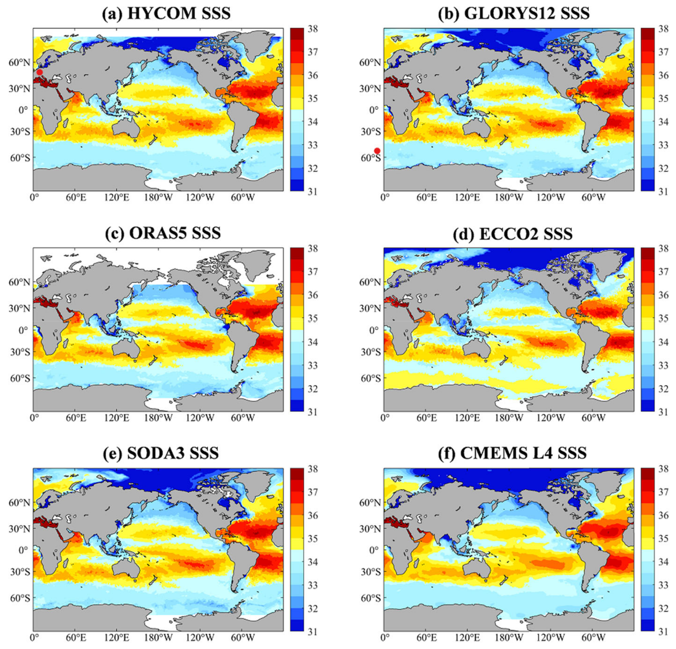
3.2. Global Assessment

Figure 6 shows the global SSS maps in June 2017 from five reanalysis and CMEMS L4 SSS product. The reason for selecting the year 2017 is that El Niño and La Niña have less influence on earth climate. The global SSS structures from five reanalysis products and in situ analyzed products are generally consistent in terms of large-scale spatial patterns, including the low salinities located in polar regions, the Eastern Indian Ocean and the East Pacific Fresh Pool (EPFP); high salinities located in the subtropical north and south Atlantic; extremely low salinity in the Baltic Sea. It is noteworthy that ocean reanalysis appears to depict a more refined SSS structure than the in situ analyzed product in open sea regions between 60° N and 60° S, which is possibly related to the high spatiotemporal resolution of reanalysis data as produced by each corresponding OGCM. Among the five reanalysis products, the ORAS5 SSS lacks the information in the Arctic due to the application of ORCA025.L75 grid configuration which excludes most areas in the Arctic. In this section, the comparison analysis of 156 months (January 2005 to December 2017) of five reanalysis SSS products is conducted at different space and time scales.
Figure 7 shows the global maps and zonal averages of mean ΔSSS from five reanalysis with respect to the CMEMS L4 SSS. The corresponding global maps of RMSD and CC values are shown in Figure 8. In tropical to subtropical regions, each reanalysis shows acceptable error (Mean bias ~0.1 PSU) away from the coast with the majority of ΔSSS values smaller than 0.3 PSU and correlation coefficients larger than 0.6 (passing the 95% significance test). Exception occurs in the ECCO2 product where the majority of global ocean is covered by large ΔSSS values, high RMSD values and low CC values. For the rest four reanalysis products, several regions with significant biases could be identified, which is similar to the validation results of satellite SSS [38,39]. Large ΔSSS values are mainly distributed along the coastlines of each continent, which is mainly attributed to the land contamination effect and the under sampling of drifting observation platforms that are either assimilated in the reanalysis products or merged by the objectively analyzed SSS. An example is the Amazon River mouth. where the mean RMSD values exceed 0.5 PSU with both positive and negative ΔSSS values located nearby. Moreover, large RMSD and low correlation coefficient values are found in the East/Japan Sea, the Bay of Bengal and the Sea of Indonesia where there are sparce in situ SSS measurements to be used for data correction. A wide range of fresher biases in the higher latitudes is partly caused by the weak association between sea ice melting and salinity variances in ocean circulation models, especially for those that are not coupled with sea-ice models. Additionally, areas with significant near surface ocean stratification also contain large differences between reanalysis and in situ measurements, such as the Eastern Pacific Fresh Pool (EPFP) where the correlation is significant with the p-values smaller than 0.05 but the ΔSSS and RMSD values are significantly larger than the open sea.
Figure 9a shows the global average of the regional temporal RMSD between reanalysis SSS and in situ analyzed SSS for the spatial scales of 0.25° × 0.25°, 1° × 1°, 3° × 3° and 10° × 10°. The RMSD values are generally consistent among SSS reanalysis data with respect to CMEMS L4 SSS. Again, the exception belongs to ECCO2 product, which presents more than twice as large as the RMSD values in all the four spatial scales. The mean RMSD decreases from ~0.23 PSU at 0.25° × 0.25° scale to ~0.12 PSU at 10° × 10° scale. This means the reanalysis SSS products show smaller differences with the in situ SSS data in larger spatial scales. The RMSD values are contributed to by the differences in time mean SSS values and differences in temporal SSS anomalies (deviation from the time mean) between reanalysis and in situ analyzed SSS. To separate the SSS differences contributed to by the time mean values and temporal anomalies, we also examine the STD of the differences between five reanalysis SSS and CMEMS L4 SSS. The time mean SSS differences do not contribute to STD values in the same way that they do to the RMSD values.
Figure 9b shows the global average STD values of SSS differences between reanalysis SSS and CMEMS L4 SSS at various spatial scales. The global mean STD values for the 0.25° × 0.25°, 1° × 1°, 3° × 3°, and 10° × 10° scales are 0.16, 0.12, 0.10, and 0.06 PSU for HYCOM, 0.19, 0.15, 0.11, and 0.07 PSU for GLORYS12, 0.19, 0.15, 0.12, and 0.07 PSU for SODA3 and 0.18, 0.14, 0.11, and 0.07 PSU for ORAS5, respectively. In contrast, the STD values for ECCO2 are significantly larger, which is attributed to the larger non-seasonal STD values. Note that the RMSD and STD values with respect to in situ analyzed SSS not only contain the errors of SSS reanalysis, but also the errors of gridded in situ SSS product. Figure 9c,d illustrates the corresponding global averaged STD values for the seasonal and non-seasonal anomalies of SSS differences between reanalysis and in situ analyzed SSS. The non-seasonal anomalies are related to the SSS differences in representing non-seasonal signals associated with phenomena such as tropical instability waves [40], El Niño-Southern Oscillation [41], Madden-Julian Oscillation [42], and Indian Ocean Dipole [43]. It is noteworthy that the global average STD values for non-seasonal SSS anomalies is significantly larger than that for seasonal SSS anomalies under each spatial scale, and the differences among SSS reanalysis is mainly reflected in the non-seasonal anomalies.

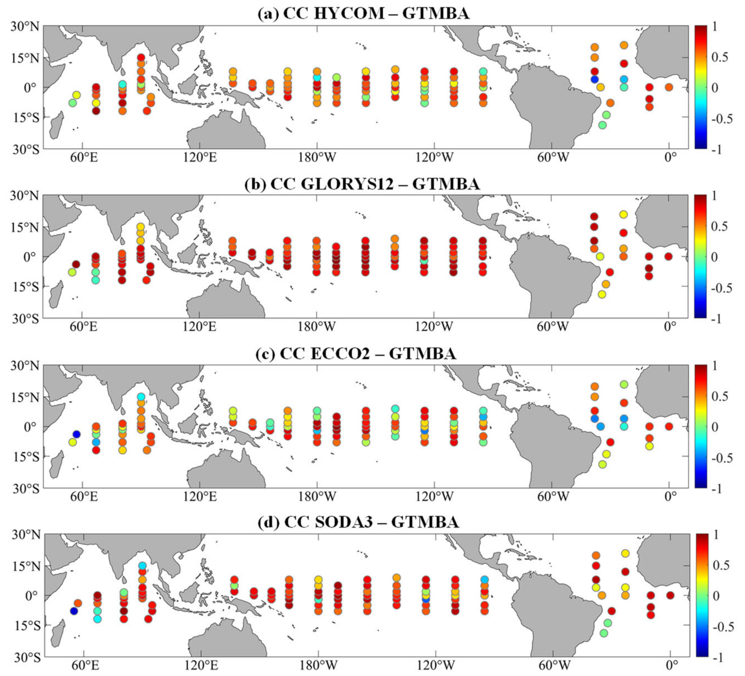
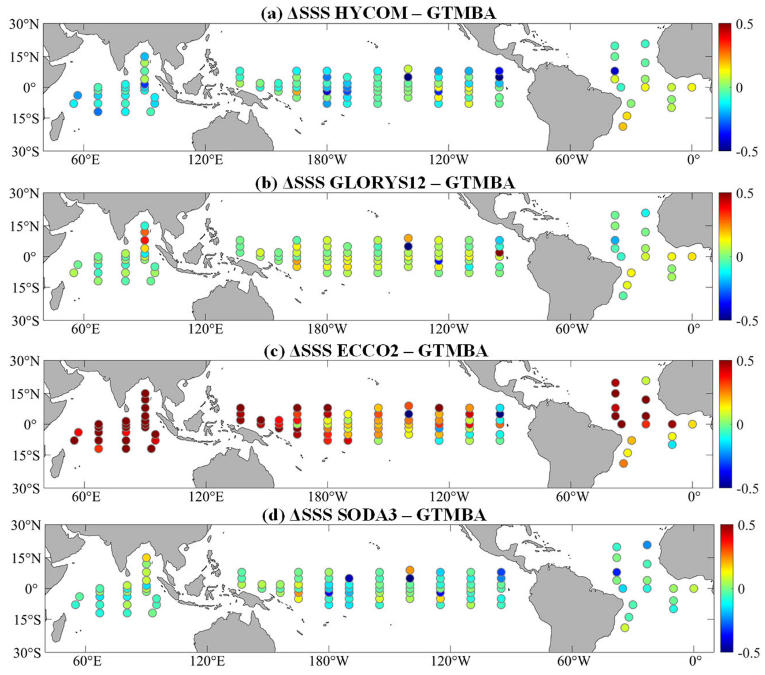
3.3. Comparison with Tropical Moored Buoys

The Global Tropical Moored Buoy Array (GTMBA) provide daily in situ SSS measurements at several fixed locations in the tropical ocean. These long-term daily sampling data are valuable for validation of reanalysis SSS data at daily to weekly scale. The weekly time series of reanalysis SSS at each buoy location were selected using the nearest grid in the 0.25° × 0.25° boxes after applying a 7-day average filtering. Note that ORAS5 product is excluded from this weekly assessment since the smallest time resolution of ORAS5 SSS is per month.
Figure 10 shows the CC values of four reanalysis SSS with respect to 1 m salinity observed by TAO buoys in the Pacific Ocean, PIRATA buoys in Atlantic and RAMA buoys in the Indian Ocean at weekly scale, respectively. The corresponding ΔSSS values are shown in Figure 11, with the RMSD values supplemented in Figure S1. We selected the time range of January 2015 to December 2015, as each buoy has more than 30 collocated weekly samples for comparison during this period. Generally, the GLORYS12 reanalysis data best agrees with the buoy salinity with the correlation coefficient exceeding 0.6 in 81% of the TAO buoys, 56% of the PIRATA buoys and 73% of the RAMA buoys, all of which has passed the significance test with p-values smaller than 0.05. SODA3 has slightly worse performance with the corresponding rates of 66% for the TAO buoys, 50% for the PRIATA buoys and 61% for the RAMA buoys. Comparatively, HYCOM and ECCO2 have further worse and generally similar performance in reproducing the weekly SSS variations in tropical ocean, especially in the Atlantic Ocean where each PRIATA buoy is labeled by consistent high and low CC values from the two reanalysis products. However, the performance represented by CC values does not exactly match that given by ΔSSS values. The lowest ΔSSS values still belong to the GLORYS12 product, whereas the largest values appear in ECCO2. HYCOM and SODA3 consistently underestimate the SSS at most locations, indicating similar capacity to reproduce the mean state of SSS in the tropical ocean, at least in the year of 2015.
Figure 12 shows the histogram of ΔSSS, RMSD and CC values between reanalysis SSS and GTMBA buoy array data, which are largely consistent with the comparison at weekly scale, except for the ECCO2 product. The ΔSSS values of each reanalysis product are mostly distributed between −0.2 to 0.2 PSU, which fundamentally follow the Gaussian distribution. Among them, HYCOM has more positive ΔSSS with buoy with a peak distribution of −0.1 PSU. In contrast the absolute majority of negative ΔSSS values are found from ECCO2 product with a peak distribution of 0.4 PSU. This agrees with the spatial comparison against CMEMS L4 SSS in tropical regions (Figure 8). The distribution of RMSD and CC between reanalysis SSS and buoy SSS also conforms to the acceptable RMSD values and high CC in tropical seas (Figure 7c). RMSD values are mainly distributed between 0.1 to 0.3 PSU with the least mean RMSD from GLORYS12 (0.21 PSU) and highest mean RMSD from ECCO2 (0.35 PSU). Similarly, the CC values are close to 1, with more than 70% values distributed between 0.5 and 1. Among four reanalysis products, GLORYS12 has the highest mean CC while ECCO2 presents the lowest value. Overall, the distribution of ΔSSS, RMSD and CC are generally consistent in each model reanalysis, among which GLORYS12 has best performance in reproducing weekly SSS states and variations in tropical ocean, and ECCO2, as similar to that found in global and regional assessment, has the worst overall data quality at weekly scale.

4. Discussion and Conclusions

In this study, the accuracy of five reanalysis SSS, generated by high-resolution ocean reanalysis systems, has been validated against in situ gridded products CMEMS L4 SSS and the tropical mooring buoys at different time and space scales. The in situ analyzed SSS product used in this study has ingested both the remotely sensed SSS from SMOS satellite and in situ SSS measurements from various platforms in CORA database. The comparison is extended to more spatial and temporal scales than some previous efforts. In situ analyzed products used in other studies are primarily based on Argo profilers, vessels and other in situ platforms, which have a low spatial coverage in coastal areas and marginal seas and can be supplied by satellite salinity merged in CMEMS L4 SSS. By comparing with in situ analyzed SSS data, we found reanalysis versus in situ RMSD generally lower than 0.5 PSU and the absolute ΔSSS values lower than 0.3 PSU. This study evaluates the SSS data quality of five state-of-the-art ocean reanalysis products for the first time, which is expected to provide reference for the study of ocean dynamics, hydrological cycle and earth climate.
The capacity of the five reanalysis products to reproduce SSS under extreme conditions is demonstrated by a multi-scale comparison in the Mediterranean Sea against the CMEMS L4 SSS, which has been used to validate multi-sensor L4 SSS in the Mediterranean Sea in previous studies [44]. We found a consistent spatial SSS structure between reanalysis SSS and in situ analyzed SSS with better performance away from the coast and gulfs. Among five reanalysis products, the HYCOM reanalysis is closest to in situ measurements. The comparison in ten subregions indicate that the performance of SSS reanalysis is not optimistic in the majority of subregions in the Mediterranean Sea. Among them, larger uncertainties are found in the Adriatic Sea, the Aegean Sea and the South Mediterranean Sea, which is mainly attributed to the under-sampling of in situ measurements used for data assimilation and objective analysis, and partly related to the contaminations and river inflow from land that were not fully considered in the ocean models. The above suggest that in such regions with bad environment for SSS reanalysis, despite a wide range of in situ salinity profiles can be used for data assimilation, some physical or empirical methods are still required to further correct the mean state and variations of reanalysis SSS, especially those generated by low resolution OGCMs. Our study also suggests the difficulty of validating reanalysis SSS at high spatiotemporal scales in marginal seas, given the paucity of in situ SSS measurements in semi-closed regions where Argo profiles are not sufficient. Perfection of an in situ observing system is crucial to improve the data quality of SSS reanalysis in marginal seas and coastal regions, which is beneficial for dynamic studies on the mesoscale salinity structures and cross-basin ocean fronts.
Through a comparison with with in situ analyzed CMEMS L4 SSS, we concluded that the SSS reproduced by reanalysis systems presents the mean bias of 0.1 PSU in open seas between 40° N and 40° S except for ECCO2 with 0.3 PSU mean ΔSSS. Several regions with large discrepancies between SMOS and in situ SSS measurements were identified, suggesting the need for an improved SSS retrieval algorithm in the future to eliminate SSS errors in coastal areas, large river mouths and EPFP region. As the spatial scale increases, the uncertainty of SSS decreases with the largest ΔSSS and RMSD values presented at 0.25° × 0.25° scale. Moreover, it is worth noting that the RMSD, STD and ΔSSS values reported in this study are not solely attributed to the SSS uncertainties in reanalysis products. The insufficient data sampling rates may also contribute to the discrepancies between reanalysis SSS and in situ SSS. It is also found that ocean reanalysis systems utilizing high resolution dynamic models tend to depict more accurate SSS structures and variations compared with those using low resolution models, suggesting that eddy-resolving ocean reanalysis products are most suitable for investigations on hydrological cycles and ocean climate.
The comparison of collocated SSS time series from four reanalysis products tropical mooring buoy data shows that GLORYS12 most accurately capture the SSS variations at weekly scales. This is probably related to the application of both 3D-Var and reduced-order Kalman filter to constrain salinity variations at higher temporal resolution. Similar to the global comparison with in situ analyzed products, regional comparison results against GTMBA buoys also comprises the statistical differences that may not only reflect the uncertainties of ocean reanalysis, but also the malfunction of buoy sensors as found by previous studies [38,39].
Finally, the new versions of ocean reanalysis and forecast products with longer time coverage, higher spatiotemporal resolution and improved data assimilation schemes will be published by various ocean institutions to provide better SSS estimations in the future, such as the 1/25° HYCOM reanalysis/analysis product under the framework of Global Ocean Forecast System 3.5 (GOFS 3.5) developed by the Naval Research Laboratory (NRL). The launch of Surface Water and Ocean Topography (SWOT) planned in December, 2022 is expected to provide higher resolution Sea Surface Height (SSH) data to better constrain the ocean circulation models, which will significantly improve the overall performance of ocean reanalysis and empowers the capacity to better identify the signatures of mesoscale ocean structures from sea surface salinity, such as eddies [45] and ocean fronts [46]. In the future, we will be able to analyze salinity changes at the global scale, with increased temporal/spatial resolution and, in turn, obtain a better understanding on their underlying link to the global hydrological cycle and climate change.

Supplementary Materials

The following supporting information can be downloaded at: https://www.mdpi.com/article/10.3390/jmse11010054/s1, Figure S1.

Author Contributions

All the authors played a critical part in the preparation of the manuscript. Conceptualization, H.W.; methodology, H.G.; software, H.W. and K.R.; validation, H.W., P.X. and K.R.; formal analysis, P.X. and H.G.; investigation, Z.Y., P.X. and H.G.; resources, H.W. and Z.Y.; data curation, H.W.; writing—original draft preparation, W.Z.; writing—review and editing, H.W., W.Z. and P.X.; visualization, W.Z.; supervision, K.R.; project administration, K.R.; funding acquisition, K.R. All authors have read and agreed to the published version of the manuscript.

Funding

The research described in this paper is carried out in the College of Meteorology and Oceanography, National University of Defense Technology. This work is supported by the National Natural Science Foundation of China under Grant No. 61901488. This work was also partially supported by the science and technology innovation program of Hunan Province under Grant No. 2022RC3070.

Data Availability Statement

All the SSS reanalysis data utilized in this study are openly and freely available. The HYCOM reanalysis and analysis product are available from https://apdrc.soest.hawaii.edu/erddap/griddap/hawaii_soest_3151_b22a_aae6.html (accessed on 1 June 2021) and https://apdrc.soest.hawaii.edu/erddap/griddap/hawaii_soest_114b_16e8_26f6.html (accessed on 1 June 2021). The GLORYS12V1 reanalysis product is available from https://resources.marine.copernicus.eu/product-detail/GLOBAL_MULTIYEAR_PHY_001_030 and the CMEMS L4 SSS is available from https://resources.marine.copernicus.eu/product-detail/MULTIOBS_GLO_PHY_NRT_015_003 (accessed on 1 January 2022). The ORAS5 reanalysis product is available from https://icdc.cen.uni-hamburg.de/thredds/catalog/ftpthredds/EASYInit/oras5 (accessed on 1 October 2022). The ECCO2 product is available from https://apdrc.soest.hawaii.edu/erddap/griddap/hawaii_soest_542a_dc69_2517.html (accessed on 1 October 2022). The SODA 3.11.2 reanalysis product is available from https://www2.atmos.umd.edu/~ocean/index_files/soda3.11.2_mn_download.html (accessed on 1 October 2022). The daily-averaged mooring buoy data are freely accessible at www.pmel.noaa.gov/tao (accessed on 1 October 2022).

Acknowledgments

We appreciate access to all the freely available products that made this study possible. These products include gridded salinity products from HYCOM, GLORYS12, ORAS5, ECCO2, SODA 3.11.2 and CMEMS L4 SSS. These products are released by the Environmental Research Division’s Data Access Program (ERDDAP) data server, the E.U. Copernicus Marine Service Information and the European Centre for Medium-Range Weather Forecasts (ECMWF).

Conflicts of Interest

The authors declare no conflict of interest.

References

  1. Ponte, R.; Vinogradova, N. An assessment of basic processes controlling mean surface salinity over the global ocean. Geophys. Res. Lett. 2016, 43, 7052–7058. [Google Scholar] [CrossRef] [Green Version]
  2. Supply, A.; Boutin, J.; Vergely, J.L.; Martin, N.; Hasson, A.; Reverdin, G.; Mallet, C.; Viltard, N. Precipitation estimates from SMOS sea-surface salinity. Q. J. R. Meteorol. Soc. 2018, 144, 103–119. [Google Scholar] [CrossRef] [Green Version]
  3. Yu, L.; Jin, X.; Josey, S.A.; Lee, T.; Kumar, A.; Wen, C.; Xue, Y. The global ocean water cycle in atmospheric reanalysis, satellite, and ocean salinity. J. Clim. 2017, 30, 3829–3852. [Google Scholar] [CrossRef]
  4. Johnson, H.L.; Cessi, P.; Marshall, D.P.; Schloesser, F.; Spall, M.A. Recent Contributions of Theory to Our Understanding of the Atlantic Meridional Overturning Circulation. J. Geophys. Res. Ocean. 2019, 124, 5376–5399. [Google Scholar] [CrossRef] [Green Version]
  5. Li, G.; Cheng, L.; Zhu, J.; Trenberth, K.E.; Mann, M.E.; Abraham, J.P. Increasing ocean stratification over the past half-century. Nat. Clim. Change 2020, 10, 1116–1123. [Google Scholar] [CrossRef]
  6. Gévaudan, M.; Jouanno, J.; Durand, F.; Morvan, G.; Renault, L.; Samson, G. Influence of ocean salinity stratification on the tropical Atlantic Ocean surface. Clim. Dyn. 2021, 57, 321–340. [Google Scholar] [CrossRef]
  7. Forget, G. Mapping ocean observations in a dynamical framework: A 2004–06 ocean atlas. J. Phys. Oceanogr. 2010, 40, 1201–1221. [Google Scholar] [CrossRef]
  8. Evans, D.G.; Toole, J.; Forget, G.; Zika, J.D.; Naveira Garabato, A.C.; Nurser, A.G.; Yu, L. Recent wind-driven variability in Atlantic water mass distribution and meridional overturning circulation. J. Phys. Oceanogr. 2017, 47, 633–647. [Google Scholar] [CrossRef] [Green Version]
  9. Johnson, G.; Lyman, J.; Boyer, T.; Cheng, L.; Domingues, C.; Gilson, J.; Ishii, M.; Killick, R.; Monselesan, D.; Purkey, S. Global oceans: Ocean heat content. state of the climate in 2017. Bull. Am. Meteorol. Soc 2018, 99, S72–S77. [Google Scholar]
  10. Balmaseda, M.A.; Mogensen, K.; Weaver, A.T. Evaluation of the ECMWF ocean reanalysis system ORAS4. Q. J. R. Meteorol. Soc. 2013, 139, 1132–1161. [Google Scholar] [CrossRef]
  11. Seo, G.-H.; Choi, B.-J.; Cho, Y.-K.; Kim, Y.H.; Kim, S. Evaluation of a regional ocean reanalysis system for the East Asian Marginal Seas based on the ensemble Kalman filter. Ocean. Sci. J. 2015, 50, 29–48. [Google Scholar] [CrossRef]
  12. Xie, J.; Bertino, L.; Counillon, F.; Lisæter, K.A.; Sakov, P. Quality assessment of the TOPAZ4 reanalysis in the Arctic over the period 1991–2013. Ocean. Sci. 2017, 13, 123–144. [Google Scholar] [CrossRef] [Green Version]
  13. Jones, R.; Renfrew, I.; Orr, A.; Webber, B.; Holland, D.; Lazzara, M. Evaluation of four global reanalysis products using in situ observations in the Amundsen Sea Embayment, Antarctica. J. Geophys. Res. Atmos. 2016, 121, 6240–6257. [Google Scholar] [CrossRef] [Green Version]
  14. Zuo, H.; Balmaseda, M.A.; Mogensen, K.; Tietsche, S. OCEAN5: The ECMWF Ocean Reanalysis System and its Real-Time Analysis Component; European Centre for Medium-Range Weather Forecasts: Reading, UK, 2018. [Google Scholar]
  15. Breivik, Ø.; Mogensen, K.; Bidlot, J.R.; Balmaseda, M.A.; Janssen, P.A. Surface wave effects in the NEMO ocean model: Forced and coupled experiments. J. Geophys. Res. Ocean. 2015, 120, 2973–2992. [Google Scholar] [CrossRef] [Green Version]
  16. Dee, D.P.; Uppala, S.M.; Simmons, A.J.; Berrisford, P.; Poli, P.; Kobayashi, S.; Andrae, U.; Balmaseda, M.; Balsamo, G.; Bauer, d.P. The ERA-Interim reanalysis: Configuration and performance of the data assimilation system. Q. J. R. Meteorol. Soc. 2011, 137, 553–597. [Google Scholar] [CrossRef]
  17. Legeais, J.-F.; Ablain, M.; Zawadzki, L.; Zuo, H.; Johannessen, J.A.; Scharffenberg, M.G.; Fenoglio-Marc, L.; Fernandes, M.J.; Andersen, O.B.; Rudenko, S. An improved and homogeneous altimeter sea level record from the ESA Climate Change Initiative. Earth Syst. Sci. Data 2018, 10, 281–301. [Google Scholar] [CrossRef] [Green Version]
  18. Storto, A.; Oddo, P.; Cipollone, A.; Mirouze, I.; Lemieux-Dudon, B. Extending an oceanographic variational scheme to allow for affordable hybrid and four-dimensional data assimilation. Ocean. Model. 2018, 128, 67–86. [Google Scholar] [CrossRef]
  19. Ballabrera-Poy, J.; Murtugudde, R.; Busalacchi, A. On the potential impact of sea surface salinity observations on ENSO predictions. J. Geophys. Res. Ocean. 2002, 107, SRF 8-1–SRF 8-11. [Google Scholar] [CrossRef]
  20. Behringer, D.; Xue, Y. Evaluation of the Global Ocean Data Assimilation System at NCEP: The Pacific Ocean. In Proceedings of the Eighth Symposium on Integrated Observing and Assimilation Systems for Atmosphere, Oceans, and Land Surface, AMS 84th Annual Meeting, Seattle, Washington, 11–15 January 2004. [Google Scholar]
  21. Uotila, P.; Goosse, H.; Haines, K.; Chevallier, M.; Barthélemy, A.; Bricaud, C.; Carton, J.; Fučkar, N.; Garric, G.; Iovino, D. An assessment of ten ocean reanalyses in the polar regions. Clim. Dyn. 2019, 52, 1613–1650. [Google Scholar] [CrossRef] [Green Version]
  22. Adani, M.; Dobricic, S.; Pinardi, N. Quality assessment of a 1985–2007 Mediterranean Sea reanalysis. J. Atmos. Ocean. Technol. 2011, 28, 569–589. [Google Scholar] [CrossRef]
  23. Hamon, M.; Beuvier, J.; Somot, S.; Lellouche, J.-M.; Greiner, E.; Jordà, G.; Bouin, M.-N.; Arsouze, T.; Béranger, K.; Sevault, F. Design and validation of MEDRYS, a Mediterranean Sea reanalysis over the period 1992–2013. Ocean. Sci. 2016, 12, 577–599. [Google Scholar] [CrossRef]
  24. Soto-Navarro, J.; Jordá, G.; Amores, A.; Cabos, W.; Somot, S.; Sevault, F.; Macías, D.; Djurdjevic, V.; Sannino, G.; Li, L. Evolution of Mediterranean Sea water properties under climate change scenarios in the Med-CORDEX ensemble. Clim. Dyn. 2020, 54, 2135–2165. [Google Scholar] [CrossRef] [Green Version]
  25. Balmaseda, M.; Hernandez, F.; Storto, A.; Palmer, M.; Alves, O.; Shi, L.; Smith, G.C.; Toyoda, T.; Valdivieso, M.; Barnier, B. The ocean reanalyses intercomparison project (ORA-IP). J. Oper. Oceanogr. 2015, 8, s80–s97. [Google Scholar] [CrossRef]
  26. Shi, L.; Alves, O.; Wedd, R.; Balmaseda, M.; Chang, Y.; Chepurin, G.; Ferry, N.; Fujii, Y.; Gaillard, F.; Good, S. An assessment of upper ocean salinity content from the Ocean Reanalyses Inter-comparison Project (ORA-IP). Clim. Dyn. 2017, 49, 1009–1029. [Google Scholar] [CrossRef] [Green Version]
  27. Barnier, B.; Brodeau, L.; Le Sommer, J.; Molines, J.-M.; Penduff, T.; Theetten, S.; Treguier, A.-M.; Madec, G.; Biastoch, A.; Böning, C.W. Eddy-permitting ocean circulation hindcasts of past decades. Clivar Exch. 2007, 42, 8–10. [Google Scholar]
  28. Jean-Michel, L.; Eric, G.; Romain, B.-B.; Gilles, G.; Angélique, M.; Marie, D.; Clement, B.; Mathieu, H.; Olivier, L.G.; Charly, R. The Copernicus global 1/12 oceanic and sea ice GLORYS12 reanalysis. Front. Earth Sci. 2021, 9, 698876. [Google Scholar] [CrossRef]
  29. Monitoring, G.; Center, F. GLORYS12 V1—Global Ocean Physical Reanalysis Product; EU Copernicus Marine Service Information: Brussels, Belgium, 2018. [Google Scholar]
  30. Carton, J.A.; Chepurin, G.A.; Chen, L. SODA3: A new ocean climate reanalysis. J. Clim. 2018, 31, 6967–6983. [Google Scholar] [CrossRef]
  31. Jackett, D.R.; McDougall, T.J.; Feistel, R.; Wright, D.G.; Griffies, S.M. Algorithms for density, potential temperature, conservative temperature, and the freezing temperature of seawater. J. Atmos. Ocean. Technol. 2006, 23, 1709–1728. [Google Scholar] [CrossRef]
  32. Zuo, H.; Balmaseda, M.A.; Tietsche, S.; Mogensen, K.; Mayer, M. The ECMWF operational ensemble reanalysis–analysis system for ocean and sea ice: A description of the system and assessment. Ocean. Sci. 2019, 15, 779–808. [Google Scholar] [CrossRef] [Green Version]
  33. McPhaden, M.J. The Tropical Atmosphere Ocean Array Is Completed. Bull. Am. Meteorol. Soc. 1995, 76, 739–741. [Google Scholar] [CrossRef]
  34. Servain, J.; Busalacchi, A.J.; McPhaden, M.J.; Moura, A.D.; Reverdin, G.; Vianna, M.; Zebiak, S.E. A pilot research moored array in the tropical Atlantic (PIRATA). Bull. Am. Meteorol. Soc. 1998, 79, 2019–2032. [Google Scholar] [CrossRef]
  35. Mcphaden, M.J.; Meyers, G.; Ando, K.; Masumoto, Y.; Murty, V.; Ravichandran, M.; Syamsudin, F.; Vialard, J.; Yu, L.; Yu, W. RAMA: The research moored array for African–Asian–Australian monsoon analysis and prediction. Bull. Am. Meteorol. Soc. 2009, 90, 459–480. [Google Scholar] [CrossRef]
  36. Kobayashi, T.; Minato, S. COARE Seacat data: Calibrations and quality control procedures COARE Seacat data: Calibrations and quality control procedures, 1999. J. Oceanogr. 2005, 61, 995–1009. [Google Scholar] [CrossRef]
  37. Taylor, K.E. Summarizing multiple aspects of model performance in a single diagram. J. Geophys. Res. Atmos. 2001, 106, 7183–7192. [Google Scholar] [CrossRef]
  38. Bao, S.; Wang, H.; Zhang, R.; Yan, H.; Chen, J. Comparison of Satellite-Derived Sea Surface Salinity Products from SMOS, Aquarius, and SMAP. J. Geophys. Res. Ocean. 2019, 124, 1932–1944. [Google Scholar] [CrossRef]
  39. Tang, W.; Fore, A.; Yueh, S.; Lee, T.; Hayashi, A.; Sanchez-Franks, A.; Martinez, J.; King, B.; Baranowski, D. Validating SMAP SSS with in situ measurements. Remote Sens. Environ. 2017, 200, 326–340. [Google Scholar] [CrossRef] [Green Version]
  40. Lee, T.; Lagerloef, G.; Kao, H.Y.; McPhaden, M.J.; Willis, J.; Gierach, M.M. The influence of salinity on tropical Atlantic instability waves. J. Geophys. Res. Ocean. 2014, 119, 8375–8394. [Google Scholar] [CrossRef]
  41. Qu, T.; Yu, J.-Y. ENSO indices from sea surface salinity observed by Aquarius and Argo. J. Oceanogr. 2014, 70, 367–375. [Google Scholar] [CrossRef] [Green Version]
  42. Grunseich, G.; Subrahmanyam, B.; Wang, B. The Madden-Julian oscillation detected in Aquarius salinity observations. Geophys. Res. Lett. 2013, 40, 5461–5466. [Google Scholar] [CrossRef]
  43. Du, Y.; Zhang, Y. Satellite and Argo observed surface salinity variations in the tropical Indian Ocean and their association with the Indian Ocean dipole mode. J. Clim. 2015, 28, 695–713. [Google Scholar] [CrossRef] [Green Version]
  44. Sammartino, M.; Aronica, S.; Santoleri, R.; Buongiorno Nardelli, B. Retrieving Mediterranean Sea Surface Salinity Distribution and Interannual Trends from Multi-Sensor Satellite and In Situ Data. Remote Sens. 2022, 14, 2502. [Google Scholar] [CrossRef]
  45. Melnichenko, O.; Amores, A.; Maximenko, N.; Hacker, P.; Potemra, J. Signature of mesoscale eddies in satellite sea surface salinity data. J. Geophys. Res. Ocean. 2017, 122, 1416–1424. [Google Scholar] [CrossRef]
  46. Yu, L. Sea-surface salinity fronts and associated salinity-minimum zones in the tropical ocean. J. Geophys. Res. Ocean. 2015, 120, 4205–4225. [Google Scholar] [CrossRef]
Figure 1. (Upper) Topography and subregions divided in the Mediterranean Sea, including zone1: Alboran Sea, zone 2: Algerian Sea, zone 3: Balearic Sea, zone 4: Tyrrhenian Sea, zone 5: Southern Mediterranean, zone 6: Adriatic Sea, zone 7: Ionian Sea, zone 8: Libyan Sea, zone 9: Aegean Sea and zone 10: Levantine Sea. (Bottom) Data volume of in situ SSS measurements in the Mediterranean Sea as obtained from profilers, buoys, glider, drifter, CTD provided by the World Ocean Database 18 and ship measurements provided by Global Ocean Surface Underway Data, which has been ingested by the CMEMS L4 SSS product.
Jmse 11 00054 g001
Figure 2. Mean SSS field in the Mediterranean Sea averaged from (a) HYCOM reanalysis, (b) GLORYS12, (c) ORAS5, (d) ECCO2, (e) SODA 3.11.2 and (f) CMEMS L4 SSS on a consistent 0.25° × 0.25° grid. The unit is in PSU.
Jmse 11 00054 g002
Figure 3. Same as Figure 1 but for the STD field. The unit is in PSU.
Jmse 11 00054 g003
Figure 4. Horizontal distribution of mean ΔSSS (left) and RMSD (right) values with respect to CMEMS L4 objective analyzed SSS. From top to bottom: HYCOM, GLORYS12, ORAS5, ECCO2 and SODA3. The unit of ΔSSS is in PSU and the CC values are unitless.
Jmse 11 00054 g004
Figure 5. Taylor diagram of monthly ocean reanalysis products versus CMEMS L4 SSS for the ten zones of the Mediterranean Sea, including (a) the Alboran Sea, (b) the Algerian Sea, (c) the Balearic Sea, (d) the Tyrrhenian Sea, (e) the South Mediterranean, (f) the Adriatic Sea, (g) the Ionian Sea, (h) the Libyan Sea, (i) the Aegean Sea, (j) the Levantine Sea. The unit is in PSU for biases and RMSDs. Statistics beyond the scope (smaller than 0 for CC, larger than 2 for normalized STD and larger than 2.5 for normalized RMSD) are not marked in the figures.
Jmse 11 00054 g005
Figure 6. Global SSS maps for (a) HYCOM, (b) GLORYS12, (c) ORAS5, (d) ECCO2, (e) SODA3 and (f) CMEMS L4 product at June 2017. The unit is in PSU.
Jmse 11 00054 g006
Figure 7. Comparison of ΔSSS in five reanalysis SSS against the CMEMS L4 SSS product, including (a) HYCOM, (b) GLORYS12, (c) ORAS5, (d) ECCO2 and (e) SODA3. (f) The zonal average of ΔSSS values from 60° N to 60° S. The unit is in PSU.
Jmse 11 00054 g007
Figure 8. Comparison of RMSDs and correlation coefficients in five reanalysis SSS against the CMEMS L4 SSS product. The unit is in PSU for RMSD values.
Jmse 11 00054 g008
Figure 9. (a) Global average of temporal RMSD values between each reanalysis product and CMEMS L4 SSS product on four spatial scales indicated by legends along the horizontal axis. Global average of temporal STD values for the differences between each reanalysis product and CMEMS L4 SSS product on four different spatial scales for (b) total anomaly, (c) seasonal anomaly and (d) non-seasonal anomaly. The RMSD and STD values are in the unit of PSU.
Jmse 11 00054 g009
Figure 10. Comparison of CC values between five SSS reanalysis products with respect to the salinity data measured by GTMBA buoys at 1 m depth at weekly scale. The time range is from 1 January 2015 to 31 December 2015.
Jmse 11 00054 g010
Figure 11. Same as Figure 10 but in terms of ΔSSS values.
Jmse 11 00054 g011
Figure 12. Histogram of ΔSSS, RMSD and CC values between HYCOM (purple), GLORYS12 (dark red), ECCO2 (yellow), SODA3 (magenta) and GTMBA buoy salinity at 1 m. (a) weekly ΔSSS, (b) weekly RMSD, (c) weekly CC values. The numbers in the top right legend are the corresponding average ΔSSS (a), RMSD (b) and CC (c) values.
Jmse 11 00054 g012
Table 1. List of ocean reanalysis products.
DatasetModelForcingGrid
Resolution
Assimilation MethodAssimilated Data
HYCOM GOFS 3.0HYCOM 2.2NCEP CFSR1/12°3D MVOISatellite SST
Altimeter SLA
Ship and buoy T/S profiles
In situ ocean currents
GLORYS12NEMO 3.1ERA-Interim1/12°3D-Var
Reduced-order
Kalman Filter
Altimeter SLA
AVHRR SST
CORA T/S profiles
SODA3MOM5DFS5.21/4°Linear Deterministic Sequential FilterWOD09 T/S profiles
Satellite SST
ICOADS SST
ECCO2MITgcmNCEP/NCAR1/4°Least Squares FitGHRSST-PP SST
WOCE T/S profiles
TAO, Argo, XBT T/S profiles
ORAS5NEMO 3.4ERA-Interim∼1/4°3D-Var FGAT
(NEMOVAR)
EN4 T/S profiles
corrected by XBT/MBT data
HadISST2 + OSTIA SST
Table 2. Algorithm for calculating fundamental statistic parameters for assessment in this study.
Statistical
Parameter
Algorithm
SSS Mean i = 1 n S S S i (1)
ΔSSS S S S r e a n a l y s i s S S S i n   s i t u (2)
STD i = 1 n ( S S S S ¯ S ¯ S ¯ ) 2 n (3)
RMSD i = 1 n ( S S S r e a n a l y s i s S S S i n   s i t u ) 2 n (4)
CC 1 i = 1 n ( S S S r e a n a l y s i s S ¯ S ¯ S ¯ r e a n a l y s i s ) ( S S S i n   s i t u S ¯ S ¯ S ¯ i n   s i t u ) i = 1 n ( S S S r e a n a l y s i s S ¯ S ¯ S ¯ r e a n a l y s i s ) 2   ( S S S i n   s i t u S ¯ S ¯ S ¯ i n   s i t u ) 2 (5)
1 The p-values of the correlation coefficient are obtained from the MATLAB toolbox with a significance level of 0.05.
Disclaimer/Publisher’s Note: The statements, opinions and data contained in all publications are solely those of the individual author(s) and contributor(s) and not of MDPI and/or the editor(s). MDPI and/or the editor(s) disclaim responsibility for any injury to people or property resulting from any ideas, methods, instructions or products referred to in the content.

