Abstract
Mathematical modelling of visco-elastic plate breaking and consequent deflection of the plate are studied using the simplified formulation. The plate is modelled as a thin visco-elastic plate of constant thickness. The edges of the plate are clamped. The plate deflection is caused by a uniform aerodynamic pressure, which slowly increases in time. The plate deflection before breaking is approximated as quasi-static. The plate breaks instantly then and there, when and where the modified fracture criterion by Petrov and Morozov is achieved. Both the deflections and velocities of the plate before and after breaking are assumed equal.The motion of the plate parts after breaking are highly unsteady and dependent on the viscous properties of the plate. If the viscosity of the plate material is negligible compared with the elastic characteristics of the plate, then the velocity of the plate deflection is discontinuous at the time instant of the plate breaking. This feature of the plate motion after its breaking should be taken into account in interpretation of the numerical results within the linearised model of plate deflection with sudden breaking. It is shown that the plate can break in a cascade way. Each part after the first breaking breaks again. The configuration studied in this paper is specially tailored to highlight the behaviour of the numerical solutions of the plate breaking problems in applications.
1. Introduction
The present study is motivated by vertical impact of a rigid body onto a floating ice floe with subsequent breaking the floe. It two-dimensional formulation, this problem was studied in [1] for visco-elastic homogeneous plate of constant thickness before the plate breaking. Korobkin and Khabakhpasheva [2] investigated the problem of vertical impact onto a floating plate with a central crack, which is normal to the plate surface. The plate was modelled as rigid outside the crack. The crack was modelled by a torsional spring. The stress intensity factor for the crack was not allowed to be greater than the ice fracture toughness. If the stress intensity factor approaches the fracture toughness value, the crack grows in such a way that the stress intensity factor is either below or equal to the fracture toughness of the plate material. The problem was reduced to a non-linear ordinary differential equation of the second order for the opening angle of the crack. The calculations were terminated when the crack length achieved 90% of the plate thickness. Recently this study was generalised to a crack in a visco-elastic thin plate. Two criteria of the plate breaking were used. These criteria are based on the concept of stress intensity factor for the crack tip and the concept of yield strain. The crack was modelled by a torsional spring as in [2,3]. Only the criterion of the plate breaking based on the concept of the yield strain of the plate material was used for cracks longer than 90% of the plate thickness. The plate was assumed to break instantly when the strain at the place of the crack achieves the yield strain value. This model of visco-elastic plate breaking is highly simplified. However, it is expected to be suitable for practical calculations of impact loads experienced by a ship navigating in icy waters and loads experienced by a lifeboat launched in water covered with ice floes. The impact loads are dependent on behaviour of ice floes during the impact and its possible breaking, see [4] for discussions. The model of ice floe breaking by vertical impact should be developed further by using laboratory experiment in well controlled conditions. We are unaware of such experiments with floating ice plates with or without pre-existing cracks for vertical impact on the plates, in contrast to extensive experimental studies of horizontal impact by ice floes onto offshore structures and ships. On the other hand, models of breaking ice floes should be simplified further in a robust way, leading to practical tools of estimating impact loads in real life situations, see [5] for general formulation of the problem.
In order to be sure that our model of vertical impact onto an ice floe with its breaking is reliable, we need to check that the numerical results provided by the model are not affected by the numerical algorithm in use. Preliminary results for the problem of rigid body impact onto a floating visco-elastic plate with account for the plate breaking into two parts obtained by the normal mode method with accurate calculations of the added mass matrices before and after the plate breaking, see [6,7], showed that the plate speed exhibits a discontinuity close to the place of the plate breaking, even though the numerical algorithm requires the plate speed continuity at the time instant of the plate breaking. The instant of the plate breaking is critical for the subsequent interaction of the impacting rigid body with the ice plate. Correct understanding of the plate motion after breaking is important for the prediction of the impact loads. To gain knowledge about the visco-elastic plate motion after its breaking, we formulate in this paper a problem which mimics the breaking process and can be solved analytically with analysis of the solution in full detail. This problem was inspired by the configuration studied in [8], where impact onto a floating plate between two vertical walls was considered.
The simplified problem of highly unsteady two-dimensional motion of a thin visco-elastic plate after the plate breaking by a uniform slowly time-varying load is formulated as follows. Initially the plate is horizontal and corresponds to the interval , , see Figure 1a. The plate edges are clamped. Then a uniform load is applied to the upper surface of the plate. One can think about a sealed air chamber above the plate, see Figure 1a, where the air pressure is gradually increased up to a certain value , at which the plate deflection and the bending stresses in the plate are so high that the plate breaks into two parts but the air chamber continues to be sealed. The load magnitude p increases slowly in time, such that the plate deflection is quasi-stationary. The plate deflection before the plate breaks is governed by the equation , where and D is the plate rigidity, with the edge conditions . The solution of this boundary problem, , is even and smooth. It is given by the formula, , where . The strains on the plate surface are given by the formula, , where h is the plate thickness. The strain magnitude is maximum at the plate edges and have its local maximum at the plate centre, . Note that .
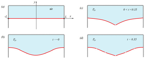
Figure 1.
Sketch of the clamped plate broken by the air pressure; (a) Initial horizontal position of the plate with the air pressure inside the chamber being equal to the external ambient pressure, (b) shape of the plate before its first breaking, (c) dynamical shape of the plate after the first breaking but before the second one, (d) the second breaking of the plate without increase of the the pressure.
The strains linearly increase with increase of the air pressure p within the linear model of plate deflection. The material of the plate is assumed brittle. According to the phenomenological failure criterion, the plate breaks suddenly then and there, when and where the strain approaches the so-called uniaxial tensile strain of the material. Note that this failure criterion depends on the value of , which does not affect the plate dynamics in elastic regime and can be different in different parts of the plate. For example, ultimate tensile strength of ice is in the range 0.7–3.1 MPa. With Young’s modulus of ice Pa, we find in the range , which well corresponds to the result by Schulson [9], who wrote “ice breaks after lengthening 0.01–0.1% through transgranular cleavage”.
To model plate breaking far from its edges, we assume that the ultimate tensile strength of the plate is constant in the central part of the plate, where , and then increase linearly towards the plate ends. The corresponding tensile strain is equal to a constant in and is , where . We assume that such non-uniform ultimate tensile strength of the plate material does not affect the plate rigidity D. Such a plate breaks at the middle, where the strains have their local maximum, but not at the support edges , where the strains are higher than at the plate centre, but the plate material is stronger. The selected tensile strain is motivated by our original problem of a plate, which is broken in its inner part but not at its edge. These types of floating ice breaking are observed under vertical impact onto an ice floe [1], floating ice interaction with sloped structures [10], and level ice failure by an icebreaker [11].
Comparing the strain at the plate centre, , with the tensile strain there, we find the critical value of the air pressure .
The time, when the air pressure achieves this critical value, is taken as . We assume that at this time instant the plate breaks instantly into two parts, and , with the edges at being free of stresses and shear force, where . We do not account here for separation of the edges. We do not account also for leakage of the air through the gap between the two parts of the plate assuming that the air chamber is sealed. The air pressure in the chamber does not change after the plate breaks. We shall determine the motion of the visco-elastic plate after its breaking. In particular, it will be shown that the plate breaks second time after the first break without increase of the air pressure. This implies that cascade mechanism of plate breaking is possible. The studied configuration and the conditions of plate breaking are highly simplified with the aim to reveal features of the plate motion after its breaking.
2. Formulation of the Problem
The plate deflection, , after breaking, , is an even function of x. We consider only the right plate, . The small deflections of this thin visco-elastic plate are governed by the equations [12,13]
where m is the mass of the plate per unit area, is a constant critical air pressure at which the plate breaks (it was determined above), and is the retardation time of the plate material. The initial conditions in the problem (1) imply that both the plate deflections and speeds are continuous at the breaking instant. Note that the plate speed before the plate breaking was negligible because of the slow time-varying pressure.
Without account for both the damping, , and a failure criterion after , the plate oscillates without decay around its static deflection. The solution of the problem (1) tends to the static deflection, , as and . The corresponding static strain distribution in the right plate is given by . The module of this strain is greater than the tensile strain of the plate material in . Therefore, within the present failure model, the static deflection cannot be achieved. The plate will break again with the time and position of the new breaking to be determined by the unsteady solution of the problem (1). After the secondary breaking, we have two free-free plates, and , and two cantilever plates, and . For each of these four plates we can formulate unsteady problems similar to (1), in order to find the motions of the plates after the secondary breaking. Third and subsequent breaks of the plate are possible in the present simplified problem, as well as in more complex problems of impact onto a floating visco-elastic plate. The problem (1) can be solved formally for any , but we should terminate the solution when the failure criterion is satisfied.
Note that the initial and boundary conditions at in the problem (1) do not match each other. This implies that the strains and deflections close to and are locally self-similar. We do not consider this interesting problem here. This observation shows that some numerical difficulties are expected near the breaking place, where derivatives of the deflections and strains both in time and along the plate can be high. Interestingly, the duration of this self-similar initial stage is proportional to the retardation time and decays as . In general, the idea that any damping makes a solution smooth, is wrong for unsteady problems, see [1], where the damping model used in (1) increases the impact loads.
It will be shown below that the plate velocity changes rapidly during an early stage just after the breaking near the free-free edge, , for small . This property of the solution should be taken into account in numerical integration in time of the plate equation just after the plate breaking. The problem (1) is solved by the method of normal modes. The solution is obtained in the form of a series, terms of which are given by analytical formulae. However, this does not help because the convergence of the series for strains is weak for any . The convergence can be improved by analysing asymptotic behaviour of the coefficients in the series. However, this technique does not work for small times of order . There are still open problems with the plate motion just after the plate breaking. Later in time, when we approach the secondary breaking, our solution allows us to investigate the plate deflection and strains in the plate and plate velocities after the plate breaking with high accuracy.
3. Solution of the Problem
The problem (1) is solved in the dimensionless variables denoted with tilde,
The dimensionless deflection satisfies the following equations (tilde is dropped below)
The solution of the problem (3) depends on a single positive parameter , which is the ratio of the retardation time and the time scale of the natural plate vibration.
The problem (3) is solved using the normal modes of a cantilever beam , which are the non-zero solutions of the spectral problem
where are the eigenvalues of the spectral problem (4), and . The modes are orthogonal and normalised as
where for and . The modes are given by
where are positive roots of the dispersion equation,
It can be shown that , , where satisfies the equation
Equation (8) is solved by iterations starting from the initial guess . Note that tends to zero exponentially as .
The initial deflection of the plate can be presented as a superposition of the normal modes,
where
Equations (6) and (10) yield
Within the normal mode method, the plate deflection is sought in the form,
with time-dependent coefficients to be determined. Substituting (12) in the plate Equation (3) and using the orthogonality condition (5), we have
where . The solutions of (13) are different for small and large n.
For small n, where , we obtain
with . For , we have
where , , . Note that and as . For , only solution (14) is used. Therefore, and as for any . This implies that the present mechanism of structural damping does not increase the rate of decay of the coefficients in (12) as .
4. Analysis of the Solution
The solution of the problem (3) depends on a single parameter of the problem . Small values of imply that the retardation time is much smaller than the time scale defined in (2). The dimensionless deflection at the breaking place of the plate, , is shown in Figure 2 as a function of the dimensionless time t for different values of the parameter . The deflections and velocities of the plate are computed with 1000 terms retained in the series (12) and the dimensionless time step . The static deflection of this edge of the plate is 1 at the time of breaking and 3 for large time, see the formulation of the problem (1). The unsteady solution (12), (14) and (15) slowly approaches the limiting value 3 for large without oscillations. For overshooting is observed. The unsteady plate deflection at arrives at the static deflection 3 at for .
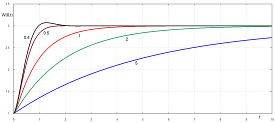
Figure 2.
Displacements of the plate edge after the plate breaking at as functions of the dimensionless time for the dimensionless retardation times .
For smaller values of the dimensionless retardation time the maximum displacement of the free edge exceed the static deflection of the edge, which is equal to 3, see Figure 3. For example, the maximum deflection of the edge for is 4 and it is achieved at . The unsteady deflection for oscillates around the static deflection with slow decay. Without damping, , the edge oscillates without decay with maximum dimensionless deflection being around 5. The speed of the plate edge quickly increases after the plate breaking to its maximum and then decays for , see Figure 4. Oscillations of the plate edges occur for . For smaller retardation times, see Figure 5, the acceleration of the plate edge after breaking increases with decrease of . An interesting effect is observed shortly after the plate breaking, see Figure 6. The velocity of the broken edge becomes discontinuous at when . Therefore, the present damping model reduces the edge acceleration after the the plate breaks. The velocities of the plate at points and as functions of the dimensionless time are shown in Figure 7 and Figure 8. Note that the velocities and displacements are positive in the direction of the external load action. It is seen that different points of the plate move in different directions during the very early stage after the plate breaks.
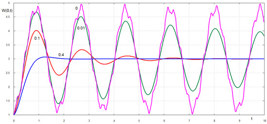
Figure 3.
Displacements of the plate edge after the plate breaking for small values of the dimensionless retardation time .
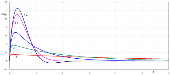
Figure 4.
Dimensionless velocity of the plate edge after the plate breaking for large values of the dimensionless retardation time .
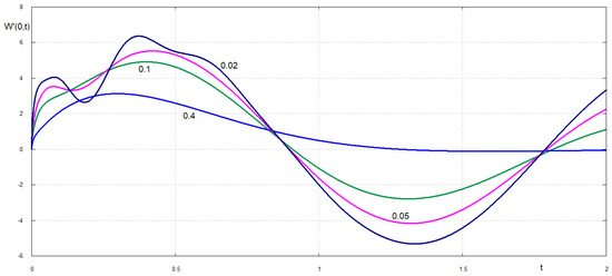
Figure 5.
Dimensionless velocity of the plate edge after the plate breaking for small values of the dimensionless retardation time .
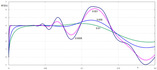
Figure 6.
Dimensionless velocity of the plate edge shortly after after the plate breaking for very small values of the dimensionless retardation time .
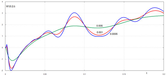
Figure 7.
Dimensionless velocity of the plate at shortly after after the plate breaking for very small values of the dimensionless retardation time .
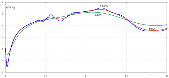
Figure 8.
Dimensionless velocity of the plate near the free-free edge, , shortly after the plate breaking for very small values of the dimensionless retardation time .
The strain in the plate after its breaking is given in the dimensionless variables by the formula
Calculations of the second derivative, , require the second derivatives of the normal modes. Note that and as . Therefore the terms in the series for and, correspondingly for the strain decay as . This means that the series for cannot be evaluated numerically without a special treatment of its convergence. Convergence of such series can be improved in several ways. In the present study we use the modified fracture criterion suggested by Petrov and Morozov [14]. They argued that the maximum values of elastic strains at a certain point of the structure and at a given time instant are not enough to conclude about a crack initiation in the structure and its following failure. They suggested that an averaged, both in time and space, strain should be used as a measure of the structural failure. The time and space intervals of averaging are related to the so-called fracture incubation time and the characteristic size l of a fracture zone, which could be reasonable to select as the plate thickness for thin plates. A review of this modified fracture criterion can be found in [1].
To demonstrate the modified fracture criterion, we select the interval of space averaging and the incubation time in the dimensionless variables. The averaged strains in the plate read
and the modified fracture criterion is
Combing Equations (12) and (16)–(18), we conclude that the plate breaks then and there, when and where the inequality
is violated. The scaled strain distributions, , along the plate, , at different time instants are shown in Figure 9 and Figure 10 for . Here and . The displacement of the plate free edge for such dimensionless retardation time is shown in Figure 3 by green line. Figure 9 illustrates quick changes in the strains after the plate break. It is seen that the solution by the normal mode method does not satisfy the condition of zero stress at up to , which is of order of . For such an initial stage, an inner solution near the free edge is required. Later, at , the strains are rather released even near the clamped edge of the plate, see blue line in Figure 9. Then the strains start to increase with rapid changes in time between and . At the fracture condition (19) is violated. This implies that at this time the plate breaks at , on the border between the weak inner part of the plate and stronger plate part near the edge, where the plate is clamped. Therefore, our solution (12) can be used only in the interval . Then the plate beaks again. We can continue our calculations of the plate motion—actually, motions of parts of the original continuous plate—by formulating boundary problems similar to (1) for the intervals and . It is possible that the plate breaks then third time near the clamped edge. The plate pieces close to the plate centre are free-free plates, which are not expected to break due to their vibrations after the secondary breaking.
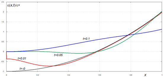
Figure 9.
Scaled strain distributions for small times after the plate breaking.
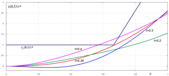
Figure 10.
Scaled strain distributions near the time instant, when the plate breaks second time.
5. Conclusions
The motion of a visco-elastic plate after it breaks into two parts has been studied using the normal mode method within the simplified model. The model allows the analytical solution of the problem but, at the same time, has main properties of the practical problems of a rigid body impact onto a floating ice floe. In this simplified problem, the plate breaks due to the air pressure, which slowly increases in time up to the plate breaking. The fracture criterion, which accounts for fracture incubation time, characteristic size of the fracture zone, and the uni-axial tensile strain of the plate material has been used. The plate breaks instantly then and there, when and where the fracture criterion is achieved. The uni-axial tensile strain was constant in the central part of the plate and then was increasing linearly towards the plate edges. It was shown that the motion of the plate after breaking depends on a single dimensionless parameter, which is the dimensionless retardation time of the plate material. If this parameter decreases, the acceleration of the plate near the breaking place increases leading to discontinuity of the plate speed in time at the breaking instant. This observation gives the idea that the obtained solution should be considered as an outer solution for small values of the dimensionless retardation time. An inner solution is required to describe the plate motion near the breaking point. The size of the vicinity of the breaking point, where the inner solution is applicable, is of the order of the dimensionless retardation time. The inner solution is expected to be self-similar. The composed solution of the present problem for small dimensionless retardation time will be studied in future work to help with the numerical solutions of elastic plate breaks in the case of materials with low viscosity. The present solution will be also generalized to other edge conditions and other loading in order to be applicable to practical problems of breaking floating ice floes.
The obtained analytical solution of the elastic plate breaking problem in the simplified formulation was investigated in detail. The analysis revealed that numerical solutions of practical problems involving breaking of elastic plates are expected to predict unbounded accelerations of the plates at the time instant of breaking. Processes with unbounded accelerations are difficult to simulate. These numerical difficulties are caused by simplified modelling of plate fracture as pure brittle.
Author Contributions
The individual contributions of the authors are specified as follows: conceptualization, A.K.; methodology, A.K. and T.K.; software, T.K.; validation, A.K. and T.K.; formal analysis A.K. and T.K.; investigation, A.K. and T.K.; resources, A.K. and T.K.; writing A.K. and T.K.; visualization, A.K. and T.K.; supervision, A.K.; project administration, A.K.; funding acquisition, A.K. All authors have read and agreed to the published version of the manuscript.
Funding
This work was supported by the NICOP research grant “Vertical penetration of an object through broken ice and floating ice plate” N62909-17-1-2128.
Institutional Review Board Statement
Not applicable.
Informed Consent Statement
Not applicable.
Data Availability Statement
Data of numerical calculations are available upon request.
Conflicts of Interest
The authors declare no conflict of interest.
References
- Khabakhpasheva, T.I.; Korobkin, A.A. Blunt body impact onto viscoelastic floating ice plate with a soft layer on its upper surface. Phys. Fluids 2021, 33, 062105. [Google Scholar] [CrossRef]
- Korobkin, A.A.; Khabakhpasheva, T.I. Impact on an ice floe with a surface crack. In Proceedings of the International Conference on Ocean, Offshore and Arctic Engineering, Madrid, Spain, 17–22 June 2018; Volume 51302, p. V009T13A014. [Google Scholar]
- Khabakhpasheva, T.I.; Korobkin, A.A. Hydroelastic behaviour of compound floating plate in waves. J. Eng. Math. 2002, 44, 21–40. [Google Scholar] [CrossRef]
- Khabakhpasheva, T.; Chen, Y.; Korobkin, A.; Maki, K. Impact onto an ice floe. J. Adv. Res. Ocean Eng. 2018, 4, 146–162. [Google Scholar]
- Korobkin, A.; Părău, E.I.; Vanden-Broeck, J.M. The mathematical challenges and modelling of hydroelasticity. Philos. Trans. R. Soc. Lond. A 2011, 369, 2803–2812. [Google Scholar] [CrossRef] [PubMed]
- Korobkin, A.A.; Khabakhpasheva, T.I. Regular wave impact onto an elastic plate. J. Eng. Math. 2006, 55, 127–150. [Google Scholar] [CrossRef]
- Khabakhpasheva, T.I.; Korobkin, A.A. Elastic wedge impact onto a liquid surface: Wagner’s solution and approximate models. J. Fluids Struct. 2013, 36, 32–49. [Google Scholar] [CrossRef]
- Korobkin, A.A.; Khabakhpasheva, T.I.; Ye, H.; Maki, K. Vertical impact onto floating ice. In Proceedings of the 25th International Symposium on Ice, Trondheim, Norway, 23–25 November 2020; pp. 473–482. [Google Scholar]
- Schulson, E.M. The structure and mechanical behavior of ice. JOM 1999, 51, 21–27. [Google Scholar] [CrossRef]
- Kerr, A.D. The bearing capacity of floating ice plates subjected to static or quasi-static loads. J. Glaciol. 1976, 17, 229–268. [Google Scholar]
- Tan, X.; Riska, K.; Moan, T. Effect of dynamic bending of level ice on ship’s continuous-mode icebreaking. Cold Reg. Sci. Technol. 2014, 106, 82–95. [Google Scholar] [CrossRef]
- Timoshenko, S. Vibration Problems in Engineering; D. van Nostrand Company: New York, NY, USA, 1937. [Google Scholar]
- Squire, V.; Hosking, R.J.; Kerr, A.D.; Langhorne, P. Moving Loads on Ice Plates; Springer Science & Business Media: Berlin/Heidelberg, Germany, 1996; Volume 45. [Google Scholar]
- Petrov, Y.V.; Morozov, N.F. On the modeling of fracture of brittle solids. J. Appl. Mech. 1994, 61, 710–712. [Google Scholar] [CrossRef]
Publisher’s Note: MDPI stays neutral with regard to jurisdictional claims in published maps and institutional affiliations. |
© 2022 by the authors. Licensee MDPI, Basel, Switzerland. This article is an open access article distributed under the terms and conditions of the Creative Commons Attribution (CC BY) license (https://creativecommons.org/licenses/by/4.0/).