A 2D Model for 3D Periodic Deep-Water Waves

Abstract

The paper is devoted to further development of an accelerated method for simulation of the two-dimensional surface waves at infinite depth with the use of a two-dimensional model derived with simplifications of the three-dimensional equations for potential periodic deep-water waves. A 3D full wave model (FWM) is based on a numerical solution of a 3D Poisson equation written in the surface-fitted coordinates for a nonlinear component of the velocity potential. For sufficient vertical resolution used for the Poisson equation, the 3D model provides very high accuracy. The simplified model is based on the 2D Poisson equation written for a free surface. This exact equation contains both the first and second derivatives of the velocity potential, i.e., it is unclosed. The analysis of the accurate solutions for the 3D velocity potential obtained with the 3D model shows that those variables are linearly connected to each other. This property allows us to obtain a 2D equation for the first derivative of the velocity potential (i.e., vertical velocity on surface), which gives the closed 2D formulation for a 3D problem of two-dimensional waves. The previously developed scheme was not universal since the parameters of the closure scheme had to be adjusted to the specific setting. The current paper offers a new formulation of a closing scheme based on the integral parameters of wave field. The method of closing the equations, as well as the numerical parameters, were chosen on the basis of the multiple numerical experiments with the full nonlinear wave model (FWM) and selection of a suitable closing scheme. That is why the given model can be called Heuristic Wave Model (HWM). The connection between the first and second variables is not precise; hence, the method as a whole cannot be exact. However, the derived 2D model is able to reproduce different statistical characteristics of the 2D wave field with good accuracy. The main advantage of the model developed is its high performance exceeding that of 3D model by about two decimal orders.

1. Introduction

A brief review of different 3D numerical methods developed for investigation of wave processes is given in [1]. Among the most advanced approaches, the following methods should be mentioned: (1) the Boundary Integral Method [2,3,4]; (2) a grid model designed at Technical University of Denmark (see [5]); (3) a High-Order Spectral (HOS) model developed at Ecole Centrale Nantes, LHEEA Laboratory [6]. A 3D model for direct simulation of periodic waves combining Fourier transform method with the finite-difference approximation in vertical for Poisson’s equation was suggested in [7] (see also [8]). The last model (we call it “Full Wave Model”, FWM) was used for simulation of wave field development under the action of the wind [9]. In the current paper, FWM for infinite depth is used as a basic model for building up a simplified model that allows for obtaining similar results at a much lower cost.

The main drawback of the 3D phase-resolving models is their low performance because all of them, one way or other, reproduce the vertical structure of wave field on the basis of a 3D equation for the velocity potential. For example, a model [1] with a resolution of $512\hspace{0.33em}\times \hspace{0.33em}513$ modes ($2048\times 1024$ knots) and just 10 vertical levels used for the simulation of wave field development over 1,200,000 time steps was running in one medium speed processor for about 45 full days. However, especially at the stage of development, the model should be run hundreds of times for validation of schemes and tuning of the parameters. Instead, just several relatively short runs before a long numerical experiment mentioned above were conducted. This is obviously not enough.

It is well known that most of the computer time for a 3D model is spent calculating the 3D structure of the velocity potential. It is necessary to emphasize that the 3D solution is used for calculation of the vertical velocity $w$ on a surface only. Unlike the 2D conformal model, a simple method of calculation of $w$ for a 3D case is not known. In the current paper, a new method of approach to the problem is suggested. The method is based on separation of the velocity potential $\phi$ into the linear $\overline{\phi }$ and nonlinear $\tilde{\phi }$ components and on consideration of Poisson’s equation for the nonlinear component on a surface. This exact equation contains both the first $\left({\tilde{\phi }}_{\zeta }=\tilde{w}\right)$ and second $\left({\tilde{\phi }}_{\zeta \zeta }={\tilde{w}}_{\zeta }\right)$ derivatives, which means that the formulation of the entire problem is not closed. However, the multiple numerical calculations with an accurate 3D model [9] showed that the vertical profiles of a nonlinear component of the velocity potential $\tilde{\phi }$ have quite a universal simple structure, which allows the suggestion that $\tilde{w}$ and ${\tilde{w}}_{\zeta }$ can be closely connected. It was shown in (10) that dependence of $\tilde{w}$ on ${\tilde{w}}_{\zeta }$ is very close to the linear one, but the coefficients in such connection depend on external integral parameters of the wave field. In the current paper, a new connection between $\tilde{w}$ and ${\tilde{w}}_{\zeta }$ with the coefficients depending on nondimensional parameters is tested. This suggestion turned out to be reliable enough to formulate the entire model that can realistically simulate wave dynamics in a broad range of external parameters.

Note that parameterization was made based on numerical experiments with 3D. FWM for infinite depth; hence, the 2-D model is suitable only for the case of infinite depth.

2. Derivation of a Simplified 2D Wave Model (HWM) for 2D Waves

The equations are written in the non-stationary surface-following non-orthogonal coordinate system:

$$\xi =x,\hspace{1em}\vartheta =y,\hspace{1em}\zeta =z-\eta \hspace{0.17em}\hspace{0.33em}\left(\xi ,\vartheta ,\tau \right),\hspace{1em}\tau =t$$

(1)

where $\eta \left(x,y,t\right) =\eta \left(\xi ,\vartheta ,\tau \right)$ is a moving periodic wave surface defined by Fourier series

$$\eta \left(\xi ,\vartheta ,\tau \right) ={\displaystyle \sum _{-M_x<k<M_x}{\displaystyle \sum _{-M_y<l<M_y}{h}_{k,l}\left(\tau \right){\Theta }_{k,l}}}$$

(2)

where k and l are the components of the vector wave number $k$, $h_{k,l}\hspace{0.17em}\left(\tau \right)$ are Fourier amplitudes for elevations $\eta \hspace{0.17em}\left(\xi ,\vartheta ,\tau \right)$, $M_x$ and $M_y$ are the numbers of modes in the directions $\xi$ and $\vartheta$, respectively, whereas ${\Theta }_{k,l}$ are the Fourier basic functions represented as a matrix:

$${\Theta }_{kl}=\left\{\begin{array}{ccc}\cos \hspace{0.17em}(k\xi +l\vartheta )& 1\le k\le M_x,& -M_y\le l<M_y\\ \cos \hspace{0.17em}(l\vartheta )& k=0,& 0\le l\le M_y\\ \sin \hspace{0.17em}(l\vartheta )& k=0,& -M_y\le l\le -1\\ \sin \hspace{0.17em}(k\xi +l\vartheta )& -M_x\le k\le -1,& -M_y\le l<M_y\end{array}\right.$$

(3)

The surface conditions for potential waves in a system of coordinates (1) at $\zeta =0$ take the following form:

$${\eta }_{\tau }=-{\eta }_{\xi }{\phi }_{\xi }-{\eta }_{\vartheta }{\phi }_{\vartheta }+\left(1+{\eta }_{\xi }^2+{\eta }_{\vartheta }^2\right){\phi }_{\varsigma }$$

(4)

$${\phi }_{\tau }=-\frac{1}{2}\left({\phi }_{\xi }^2+{\phi }_{\vartheta }^2-\left(1+{\eta }_{\xi }^2+{\eta }_{\vartheta }^2\right){\phi }_{\zeta }^2\right)-\eta -p$$

(5)

where $\phi$ is the velocity potential. Laplace equation for $\phi$ at $\zeta \le 0$ turns into the Poisson equation

$${\phi }_{\xi \xi }+{\phi }_{\vartheta \vartheta }+{\phi }_{\zeta \zeta }=\Upsilon \left(\phi \right),$$

(6)

where $\Upsilon$ is the operator:

$$\Upsilon (\hspace{0.17em})=2{\eta }_{\xi }{(\hspace{0.17em})}_{\xi \zeta }+2{\eta }_{\vartheta }{(\hspace{0.17em})}_{\vartheta \zeta }+\left({\eta }_{\xi \xi }+{\eta }_{\vartheta \vartheta }\right){(\hspace{0.17em})}_{\zeta }-\left({\eta }_{\xi }^2+{\eta }_{\vartheta }^2\right){(\hspace{0.17em})}_{\zeta \zeta }.$$

(7)

Strictly speaking, Equations (4)–(6) should be solved jointly, but since the Fourier amplitudes ${\left|h\right|}_{k,l}\left(\tau \right) ={\left(h_{k,l}^2+h_{-k,-l}^2\right)}^{1/2}$ for elevation and ${\left|\phi \right|}_{k,l}\left(\tau \right) ={\left({\phi }_{k,l}^2+{\phi }_{-k,-l}^2\right)}^{1/2}$ for the surface velocity potential change slowly, some sort of time-splitting scheme is used: Equations (4) and (5) are used as evolutionary equations for $\eta$ and $\phi$, whereas Equations (6) and (7) are used to satisfy the continuity conditions. It is accepted that in the process of the solution of Equation (7) the coefficients depending on $\eta$ are constants. Introducing the correction of $\eta$ and $\phi$ s with Equations (4) and (5) in the course of solution does not provide any advantages.

Equations (4)–(7) are written in a non-dimensional form by using the following scales: length L, where 2πL is a dimensional period in a horizontal direction; time ${\left(L/g\right)}^{1/2}$ (g is the acceleration of gravity) and the velocity potential $L^{3/2}{g}^{1/2}$. The pressure is normalized by water density so that the pressure scale is Lg. Equations (4)–(6) are self-similar to transformation with respect to L. The dimensional size of the domain is $2\pi L\times 2\pi L{M}_y/M_x$. All of the results presented in this paper are nondimensional.

It is suggested in [7] that it is convenient to represent the velocity potential as a sum of two components: an analytical (‘linear’) component $\overline{\phi }$ and an arbitrary (‘non-linear’) component $\tilde{\phi }$:

$$\phi =\overline{\phi }+\tilde{\phi }.$$

(8)

The analytical component $\overline{\phi }$ satisfies Laplace equation:

$${\overline{\phi }}_{\xi \xi }+{\overline{\phi }}_{\vartheta \vartheta }+{\overline{\phi }}_{\zeta \zeta }=0,$$

(9)

with the known solution:

$$\overline{\phi }(\xi ,\vartheta ,\zeta ,\tau )={\displaystyle \sum _{k,l}{\phi }_{k,l}(\tau )\exp \left(\mathrm{k}\zeta \right)\hspace{0.33em}}{\Theta }_{k,l},$$

(10)

where $\mathrm{k}={ \left(k^2+l^2\right)}^{1/2}$, ${\phi }_{k,l}$ are Fourier coefficients for the surface potential $\overline{\phi }$ at $\zeta =0$. The 3D solution of (9) satisfies the following boundary conditions for the surface and at infinite depth:

$$\begin{array}{l}\varsigma =0:\hspace{1em}{\overline{\phi }}_0=\phi \\ \varsigma \to -\infty :\hspace{1em}{\overline{\phi }}_{\zeta }\to 0\end{array}$$

(11)

The presentation (8) is not used for solution of evolutionary Equations (4) and (5), because it does not provide any noticeable improvements of accuracy and speed of the calculations.

The nonlinear component satisfies an equation:

$${\tilde{\phi }}_{\xi \xi }+{\tilde{\phi }}_{\vartheta \vartheta }+{\tilde{\phi }}_{\zeta \zeta }=\Upsilon \left(\phi \right),$$

(12)

Note that the full potential $\phi$ on the surface is used as a boundary condition for a linear component, so, a nonlinear component $\tilde{\phi }$ on the surface is equal to 0. Thus, Equation (12) is solved with the boundary conditions:

$$\begin{array}{l}\varsigma =0:\hspace{1em}\tilde{\phi }=0\\ \varsigma \to -\infty :\hspace{1em}{\tilde{\phi }}_{\zeta }\to 0.\end{array}$$

(13)

Hence, on the surface $\zeta =0$ Equation (12) takes the form:

$${\tilde{\phi }}_{\zeta \zeta }=\Upsilon \left(\tilde{\phi }\right)+\Upsilon \left(\overline{\phi }\right)$$

(14)

The derivatives of a linear component $\overline{\phi }$ in (7) are calculated analytically. A method of solution combines a 2D Fourier transform method in the ‘horizontal surfaces’ and a second-order finite-difference approximation on the stretched staggered vertical grid providing high accuracy in the vicinity of the surface. An Equation (12) in FWM is solved as Poisson equations with iterations over the right-hand side by the TDMA method [10] with the prescribed accuracy. The number of iterations depends on a maximum of the local surface steepness, and for high steepness it does not exceed three.

A 3D model described above is potentially exact. Its only drawback is a low speed of performance. Below is a scheme that at a cost of minor loss of accuracy provides a significantly higher speed of calculation.

Since $\tilde{\phi }\left(0\right)=0$, an Equation (12) for the velocity potential at $\zeta =0$ takes the form:

$${\tilde{w}}_{\zeta }=2({\eta }_{\xi }{w}_{\xi }+2{\eta }_{\vartheta }{w}_{\vartheta })+\Delta \eta w-s{w}_{\zeta }.$$

(15)

Here, the symbols $\Delta ={\left(\hspace{0.33em}\right)}_{\xi \xi }+{\left(\hspace{0.33em}\right)}_{\vartheta \vartheta }$ and $s={\eta }_{\xi }^2+{\eta }_{\vartheta }^2$ are used. It is remarkable that an Equation (15) is exact. From Equation (14) it follows that

$${\tilde{w}}_{\zeta }=2{\eta }_{\xi }\left({\overline{w}}_{\xi }+{\tilde{w}}_{\xi }\right)+2{\eta }_{\vartheta }\left({\overline{w}}_{\vartheta }+{\tilde{w}}_{\vartheta }\right)+\Delta \eta \left(\overline{w}+\tilde{w}\right)-s\left({\overline{w}}_{\zeta }+{\tilde{w}}_{\zeta }\right),$$

(16)

hence, Equation (15) can be represented as follows:

$$\left(1+s\right){\tilde{w}}_{\zeta }=2\left({\eta }_{\xi }{\tilde{w}}_{\xi }+{\eta }_{\vartheta }{\tilde{w}}_{\vartheta }\right)+\Delta \eta \tilde{w}+\overline{r},$$

(17)

where the term $\overline{r}$ depends only on a linear component $\overline{\phi }$:

$$\overline{r}=2\left({\eta }_{\xi }{\overline{w}}_{\xi }+{\eta }_{\vartheta }{\overline{w}}_{\vartheta }\right)+\Delta \eta \overline{w}-s{\overline{w}}_{\zeta }$$

(18)

which is calculated analytically using Fourier presentation (10) by the formulas:

$$\overline{w}(\xi ,\vartheta ,\zeta )={\displaystyle \sum _{k,l}\mathrm{k}{\phi }_{\mathrm{k},l}\exp \left(\mathrm{k}\zeta \right)}{\Theta }_{k,l},$$

(19)

$${\overline{w}}_{\zeta }(\xi ,\vartheta ,\zeta )={\displaystyle \sum _{k,l}{\mathrm{k}}^2{\phi }_{k,l}\exp \left(\mathrm{k}\zeta \right)}{\Theta }_{k,l}$$

(20)

$${\overline{w}}_{\xi }(\xi ,\vartheta ,\zeta )=-{\displaystyle \sum _{k,l}k\mathrm{k}{\phi }_{-k,-l}\exp \left(\mathrm{k}\zeta \right)}{\Theta }_{k,l},$$

(21)

$${\overline{w}}_{\vartheta }(\xi ,\vartheta ,\zeta )=-{\displaystyle \sum _{k,l}l\mathrm{k}{\phi }_{-k,-l}\exp \left(\mathrm{k}\zeta \right)}{\Theta }_{k,l}$$

(22)

The presence of ${\tilde{w}}_{\zeta }$ in Equation (17) makes the system of equations unclosed. Previously, the author regarded a surface condition (17) as a means of validation of the numerical scheme for the 3D Full Wave Model (FWM) based on a numerical solution of an equation for the velocity potential (see example of such calculation in [8]). This validation is not trivial since $w_{\zeta }$ is not a direct product of the Poisson equation solution. The finite-difference derivatives $\tilde{w}={\tilde{\phi }}_{\zeta }$ and ${\tilde{w}}_{\zeta }={\tilde{\phi }}_{\zeta \zeta }$ after solution of the 3D equation for a nonlinear component of the velocity potential were calculated as follows:

$$\tilde{w}={\tilde{\phi }}_{\zeta }\left(\zeta =0\right)=D^{-1}\left({\zeta }_2^2{\tilde{\phi }}_1-{\zeta }_1^2{\tilde{\phi }}_2\right),$$

(23)

$${\tilde{w}}_{\zeta }={\tilde{\phi }}_{\hspace{0.17em}\zeta \zeta }\left(\zeta =0\right)=2D^{-1}\left(-{\zeta }_{\hspace{0.17em}2}\hspace{0.33em}{\tilde{\phi }}_1+{\zeta }_{\hspace{0.17em}1}\hspace{0.33em}{\tilde{\phi }}_2\right).$$

(24)

Here, $D={\zeta }_1{\zeta }_2^2-{\zeta }_2{\zeta }_1^2$, ${\zeta }_i$ is depth where ${\phi }_i$ is located, ${\zeta }_0=0$, the thickness of layer ${\Delta }_i={\zeta }_i-{\zeta }_{i+1}$ grows exponentially with depth $\zeta$: ${\Delta }_{i+1}=\gamma {\Delta }_i$, whereas the value of ${\Delta }_0$ is calculated from the condition ${\displaystyle \sum _{i=0}^{i=L-1}{\Delta }_i=H}$ where $L$ is the number of levels, and $H=4\pi /{\mathrm{k}}_p$ is depth of the domain (${\mathrm{k}}_p$ is a wave number of a mode with the largest amplitude).

Since a relation (17) formally follows from the Poisson equation, the agreement between these values characterizes accuracy of the simplified scheme. The agreement cannot be very precise since the variables ${\tilde{w}}_{\zeta }$ and $\tilde{w}$ are not a direct product of the solution, and they are calculated by the approximations (23) and (24) following the solution of the Poisson equation. Moreover, the approximations for solution of the Poisson equation and calculation (23) and (24) are different. However, the calculations of ${\tilde{w}}_{\zeta }$ on the basis of Poisson Equation (12) with the approximations (23) and (24) and calculations by a surface condition (17) showed a very good agreement (see Figure 1 in [9]), which prompted us to carry out further analysis of Equation (18).

It was found that variables $\tilde{w}$ and ${\tilde{w}}_{\zeta }$ turned out to be well connected to each other. Firstly, the simplest linear hypothesis was tested:

$$\tilde{w}=A_0+A_1{\tilde{w}}_{\zeta }$$

(25)

where $A_0$ and $A_1$ are constants. This dependence was considered in [11] with the use of the 3D FWM model (described in [1,7,8,9]) that calculates the 3D structure of the velocity potential as well as 2D fields of $\tilde{w}$ and ${\tilde{w}}_{\zeta }$. The dependence between $\tilde{w}$ and ${\tilde{w}}_{\zeta }$ can be studied in Fourier space as well as in a physical space. The results obtained in Fourier space turned out to be far less certain than in a physical space, i.e., the dependence between the Fourier coefficients for $\tilde{w}$ and ${\tilde{w}}_{\zeta }$ showed considerable scatter. In our opinion, it happens because the medium and high wave numbers of Fourier amplitudes are generally unstable, whereas the verticals structure of a physical layer involved in orbital movement is universal because it is composed of a large number of modes.

The calculations performed in [11] were repeated here at a higher grid resolution $2048\times 1024$ and a number of vertical levels equal to 50. The dispersion of surface elevation $\sigma$, as well as the integral steepness s, variate in the ranges $\left(0.033<\sigma <0.066\right)$ and $\left(0.02<s<0.20\right)$, respectively. The fields included $1.7·{10}^8$ pairs of values $\tilde{w}$ and ${\tilde{w}}_{\zeta }$. 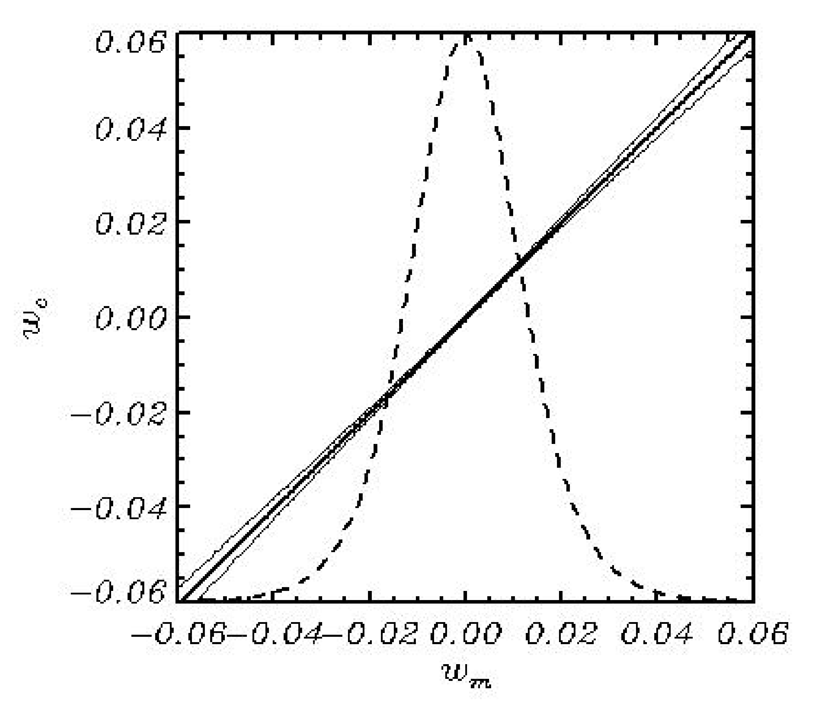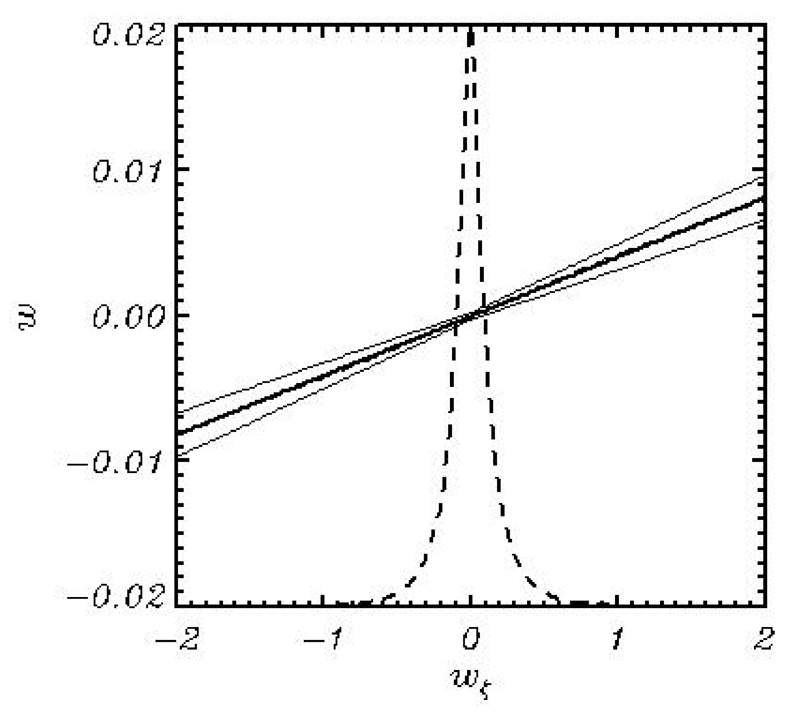The statistical connection between those variables is shown in Figure 1. It is important to underline that dependence (25) is valid for the entire wave field, i.e., the parameters $A_0$ and $A_1$ are close to constants. Otherwise, the whole approach based on a hypothesis (25) might be incorrect.

The data used for analysis included the 3D velocity potential fields $\tilde{\phi }\left(\xi ,\vartheta ,\zeta ,\tau \right)$ and the values of $\tilde{w}$ and ${\tilde{w}}_{\zeta }$ calculated by (23); the values of ${\tilde{w}}_{\zeta }$ calculated by a relation (17) and some other characteristics (see below). Since a high value of $\gamma =1.25$ for generation of vertical grid was used, the accuracy of calculation of the derivatives (23) and (24) was very high. The comparison with the analytical values of the derivatives shows that the errors of approximation (23) and (24) do not exceed ${10}^{-10}$.

The surface values of $\tilde{w}$ and ${\tilde{w}}_{\zeta }$ are defined by an asymptotic behavior of a nonlinear component of the velocity potential $\tilde{\phi }$ at $\zeta \to 0$. Hence, the connection between them can be found in the close vicinity of $\zeta =0$.

A dimensional form of (25) is

$$W=L(A_0+A_1)W_{\zeta },$$

(26)

where $W$ and $W_{\zeta }$ are dimensional analogues of $\tilde{w}$ and ${\tilde{w}}_{\zeta }$, whereas $L$ is the external scale of the problem. Formally, for any specific wave field which is more or less horizontally homogeneous, the dependence (25) is correct at appropriate choice of coefficients. However, the problem is that for different wave fields (for example, for different stages of wave field development) the variability of those coefficients can be significant. It happens because the scaling with external scale $L$ does not reflect the internal properties of wave field. To provide a more universal approximation, it is necessary to introduce the scaling in terms of integral characteristics of a given wave field with no use of $L$.

For evaluation of connection between $\tilde{w}$ and ${\overline{w}}_{\zeta }$, ten thousand short-term numerical experiments with FWM were performed. The Fourier resolution is equal to $\left(257\times 257\right)$ modes; the number of levels for solution of Poisson equation equals 30, whereas a stretching coefficient $\gamma =1.25$. The initial conditions for elevation were calculated on the basis of JONSWAP spectrum [12] for the inverse wave age $U/c_p=1$($U$ is wind velocity, $c_p$ is the phase velocity in peak of spectrum). The calculations were carried out for different values of peak wave numbers in the range $10\le k_p\le 100$. The data collected are characterized by the nondimensional dispersion of elevation

$$\sigma ={\left(\overline{{\left(\eta -\overline{\eta }\right)}^2}\right)}^{1/2},$$

(27)

in the range $\left(0.003<\sigma <0.0075\right)$ and by steepness

$$s_t={\left({\displaystyle \sum _{k,l}{\mathrm{k}}^2{S}_{k,l}}\right)}^{1/2}$$

(28)

in the range $\left(0.05<s_t<0.15\right)$ and by dispersion of Laplacian $\mathsf{\Lambda }=\Delta \eta$

$${\sigma }_L={\left(\overline{{\left(\mathsf{\Lambda }-\overline{\mathsf{\Lambda }}\right)}^2}\right)}^{1/2}$$

(29)

in the range $\left(6<{\sigma }_L<12\right)$. The calculations performed with such wide variations of integral parameters showed that the values $A$ variate in the range $\left(0.0010<A<0.0065\right)$, whereas the dependence of $w$ on $w_{\zeta }$ is not linear as assumed in [11]. Hence, the problem is reduced to finding the dependence

$$A=\frac{w}{w_{\zeta }}=f(\sigma ,{\sigma }_L,s_t\dots )$$

(30)

In fact, several additional parameters were tested, whereas $\sigma$ (Equation (27)) and ${\sigma }_L$ (Equation (29)) only turned out to be well connected with the ratio $w/w_{\zeta }$.

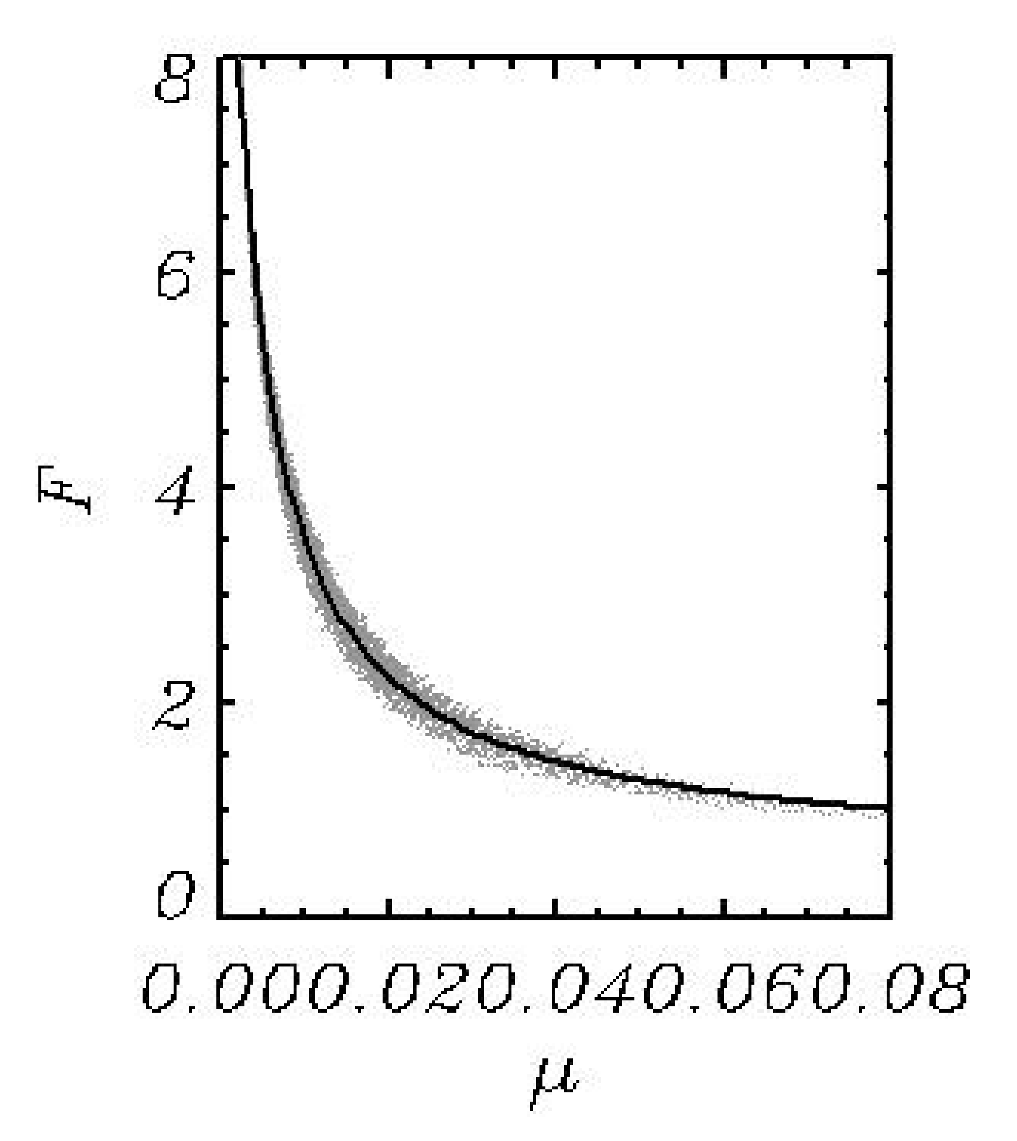
For generalization of the linear dependence (25) it is necessary to choose at least two parameters with a dimension of length taking into account internal characteristics of a wave field type (27)–(29). Finally, the best results were obtained in the following form

$$A=F(\mu ),$$

(31)

where $\mu$ is a parameter

$$\mu =\sigma \hspace{0.17em}{\sigma }_L,$$

(32)

and function $F$ is approximated by a formula

$$F=\frac{d_0\mu +d_1}{\mu +d_2},$$

(33)

where $d_0=0.535,\hspace{0.33em}{d}_1=0.0414,\hspace{0.33em}{d}_2=0.00321$ The function $F\left(\mu \right)$ is shown in Figure 2.

An approximation (33) is also correct for dimensional variables, because it is independent of the external scale $L$. The form of relation (31) and (32) and the constants in (33) were found on the basis of numerous numerical experiments with FWM (Equations (4)–(6)) and empirical selection of nondimensional variables, as well as functions and numerical parameters. That is why such simplified model is called the Heuristic Wave model (HWM).

The two-dimensional model, which is presumably able to replace the full 3D model, (4), (5), and (12), looks as follows:

$${\eta }_{\tau }=-{\eta }_{\xi }{\phi }_{\xi }-{\eta }_{\vartheta }{\phi }_{\vartheta }+\left(1+s\right)w,$$

(34)

$${\phi }_{\tau }=-\frac{1}{2}\left({\phi }_{\xi }^2+{\phi }_{\vartheta }^2-\left(1+s\right)w^2\right)-\eta -p$$

(35)

$$\tilde{w}=\frac{A\left(2\left({\eta }_{\xi }{w}_{\xi }+{\eta }_{\vartheta }{w}_{\vartheta }\right)+\Delta \eta w-s{\overline{w}}_{\zeta }\right)}{1+s}.$$

(36)

Note that the right-hand side of Equation (36) contains full vertical velocity $w=\overline{w}+\tilde{w}$ as well as a linear component of vertical velocity $\overline{w}$. An equation is represented in a form that is convenient for iterations. The iterations were performed until the next condition was reached.

$$\max \left|{\tilde{w}}^i-R^{i-1}\right|<{10}^{-7},$$

(37)

where $R$ is the right-hand side of Equation (36), whereas $i$ is the number of iterations. In the majority of cases, the number of iterations was equal to two and never exceeded four. Note that fulfilment of condition (37) can be regulated by an appropriate choice of parameters in the breaking algorithm (see below).

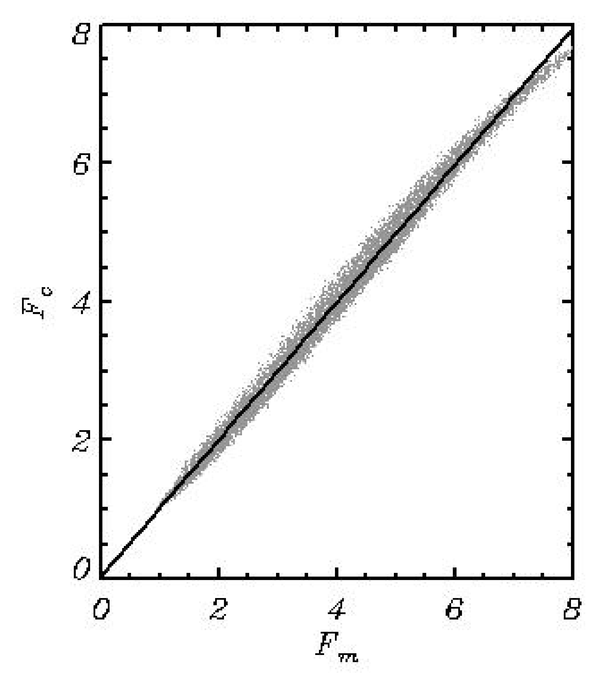
A comparison of function $F$ calculated in the course of simulation by FWM with the results of calculations by Formula (33) is given in Figure 3. The agreement between these functions is quite satisfactory: a correlation coefficient between the model values $F_m$ and those calculated by Equations (31)–(33) is equal to 0.989, the root-mean-square difference between them equal to 0.014.

In fact, the research described in this paper was initiated due to the fact discovered in the first version of the model [11]. It was found that a nonlinear component of vertical velocity $\tilde{w}$ (which is normally taken from solution of the Poisson equation) is a small value as compared with a full component $w$. However, the evolutionary Equations (34) and (35) contain a full component $w=\overline{w}+\tilde{w}$ only. It is illustrated in Figure 4 by comparison of the cumulative probability both for the full component $w$ and the nonlinear components $\tilde{w}$ (in Figure 4 they are marked as $w_t$ and $w_n$, respectively). On the average, $\tilde{w}$ is by one decimal order smaller than $w$. The main idea of the current approach is to replace the cumbersome algorithm for calculation of the vertical velocity equation $\tilde{\phi }$ with a simple 2D Equation (36). Such trick reduces the total 3D problem to the 2D one, which saves us from the endless problems associated with solving Poisson equations numerically, as well as from any other ways of reproduction of 3D structure of the velocity potential. It allows us to create a model running much faster than the 3D model.

The most convincing is the comparison of two independent methods of calculation of vertical velocity $w$, i.e., a method based on solution of Poisson Equation (12) (marked as $w_m$) and another one—based on the surface condition (36) and Equations (31)–(33) (marked as $w_c$). That comparison is given in Figure 5. The number of pairs of $w_m$ and $w_c$ used is $2\cdot {10}^9$. The root-mean-square difference between $w_m$ and $w_c$ is equal to 0.0017.

The question is how well these simplified equations reproduce wave dynamics.

A simplified model is developed on the basis of the ‘exact’ model, both models having a similar structure and a set of parameters. The evolutionary equations of both models (4), (5), (34) and (35) are essentially the same. The difference between the models is determined by the simplified calculation of small nonlinear correction to the full vertical velocity introduced by Equations (31) and (33). A straightforward way of validation of the simplified model is performing the runs with the identical setting and initial conditions. A simple case of a quasi-stationary regime was considered.

The similarity of the models can be illustrated by difference $D\left(t\right)$ (t is time)

$$D(t) = {\left({\sigma }_f^2+{\sigma }_a^2\right)}^{-1}\overline{{\left({\eta }_{i,j}^f-{\eta }_{i,j}^a\right)}^2}$$

(38)

and a correlation coefficient $C\left(t\right)$ between the fields of elevation generated by a full model

$$C(t) = {\left({\sigma }_f^2{\sigma }_a^2\right)}^{-1/2}\overline{{\eta }_f{\eta }_a}$$

(39)

where ${\sigma }_f$ and ${\sigma }_a$ are dispersions of the fields ${\eta }_f$ and ${\eta }_a$; the over-line denotes the averaging over the entire field. The right hand-sides of (38), (39) are calculated with the time interval equal to $100\Delta t$. The evolution of $D$ and $C$ given in Figure 6 shows that the fields preserve their closeness well up to $t=100$ (10,000 time steps). Such a result turned out to be quite unexpected because such a close agreement was observed for large wave fields composed of thousands of nonstationary and dispersing Fourier modes. The comparison of FWM with a simplified model was also made in [11], Figure 5. Both models used the spectral resolution of $129\times 129$ Fourier modes and $512\times 256$ knots. In the initial conditions JONSWAP spectrum with the peak wave number $k_p=30$ is assigned. It was obtained that the evolution of a correlation coefficient and a root-mean-square difference between the elevation fields was quite similar to those shown in Figure 6. Figure 6 proves that both models launched with the same boundary conditions produce a similar development for hundreds of wave peak periods. The advantage of a new scheme (Equations (31)–(33)) is its applicability to a wide range of external parameters.

The same comparison was made for FWM and HWM with a zero nonlinear correction to the vertical velocity $\tilde{w}$, i.e., using no Equation (36). The run was quite stable but an agreement between FWM and such fastest version of a simplified model was observed at a two- or three-times shorter period. Essentially, it is not clear what is more responsible for the nonlinearity: either the presence of nonlinear terms in the evolutionary Equations (34) and (35), or introducing a nonlinear correction to the vertical velocity through the exact Equation (12) or a simplified algorithm ((31)–(33) and (36)).

3. An Example of Simulation of the Wave Field Development on the Basis of HFM

The comparison of the long-term simulations performed with FWM and HWM was made in a previous publication [11]. That comparison proves that the accelerated and full models give the results quite similar to each other. The statistical characteristics of the solution were particularly well reproduced.

In the current work the calculations were performed with HWM model with the initiated algorithms for input and dissipation of energy. The algorithms for calculation of those terms are described in detail in [1,7,8,9]. The last minor modification of an algorithm for breaking is carried out in [10]. Those algorithms are not described in the current paper.

The model uses $257\times 257$ Fourier modes or $1024\times 512$ knots. The number of degrees of freedom (a minimum number of Fourier coefficients for elevation $\eta$ and the surface velocity potential $\phi$) is 264,196. In the initial conditions the JONSWAP spectrum [12] with a peak wave number ${\mathrm{k}}_p=100$ and the angle distribution proportional to ${\left(\mathrm{sch}\left(\psi \right)\right)}^{256}$ was assigned. It corresponds to nearly unidirected waves with very small energy. Note that the details of the initial conditions assigned at sufficiently high wave numbers are not important, since the model quickly develops its own wave spectrum.

The model, as well as FWM, is supplied with a developed system of algorithms for monitoring the solution and recording many functions in a spectral and grid form. The most important were the spectra of elevation and different terms describing input and dissipation of energy. An exact expression for total kinetic energy of wave motion $E_k$ in the surface-following coordinates (1) can be represented in terms of surface variables $\phi$ and $w={\phi }_{\zeta }$:

$$E_k=0.5\overline{\left(\left(1+s\right)\phi \hspace{0.17em}w+2\left({\eta }_{\xi }\phi \hspace{0.17em}{\phi }_{\xi }+{\eta }_{\vartheta }\phi \hspace{0.17em}{\phi }_{\vartheta }\right)+\Delta \eta \hspace{0.17em}{\phi }^2\right)}$$

(40)

where a single bar denotes the averaging over the $\xi$ and $\vartheta$ coordinates. A relation (40) is easily derived with a use of Poisson Equation (7) and an expression for kinetic energy written in the coordinates (1). The total potential energy $E_p$ is simply calculated by the formula

$$E_p=0.5\overline{{\eta }^2},$$

(41)

An equation of the integral energy $E=E_p+E_k$ evolution can be represented in the following form:

$$\frac{dE}{dt}=\overline{I}+\overline{D_b}+\overline{D_t}+\overline{N}$$

(42)

where $\overline{I}$ is the integral input of energy from wind; $\overline{D_b}$ is a rate of energy dissipation due to wave breaking; $\overline{D_t}$ is a rate of energy dissipation due to filtration of the high-wave number modes (‘tail dissipation’); $\overline{N}$ is the integral effect of the nonlinear interactions described by the right-hand side of the equations when the surface pressure $p$ is equal to zero. The differential forms for calculation of energy transformations can be, in principle, derived from Equations (4)–(6), but here a more convenient and simple method is applied. Different rates of the integral energy transformations can be calculated in the process of integration. For example, the value of $\overline{I}$ is calculated by the following relation:

$$\overline{I}=\frac{1}{\delta t}\left(E^{t+\delta t}-E^t\right),$$

(43)

where $E^{t+\delta t}$ is the integral energy of a wave field obtained after one time step with the right hand-side of Equation (35) containing only the surface pressure. This method is also applicable to the calculation of 1D spectra (i.e., the averaged over lateral wave number or along the direction in the polar coordinates) of different characteristics (see [1]).

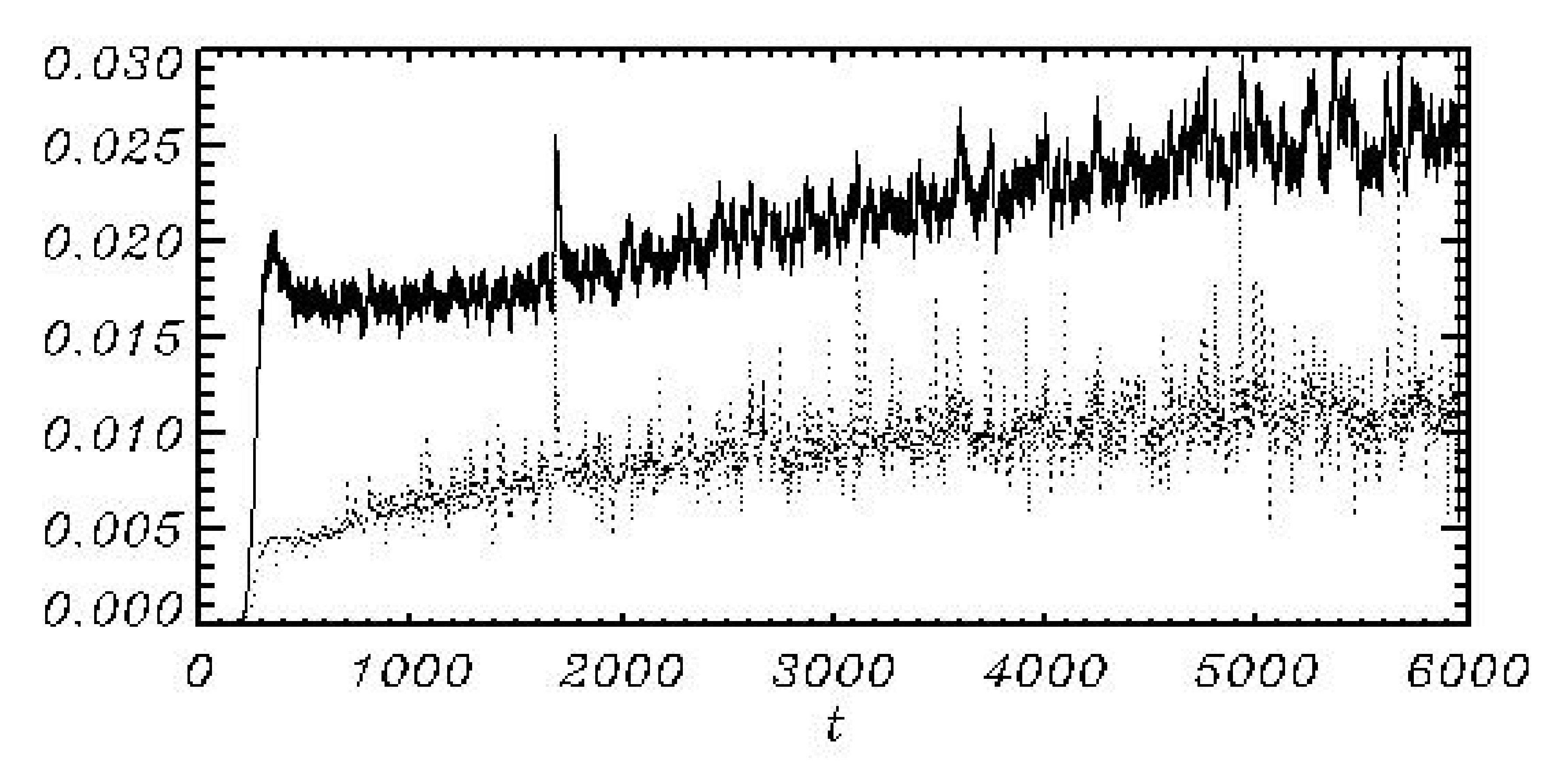
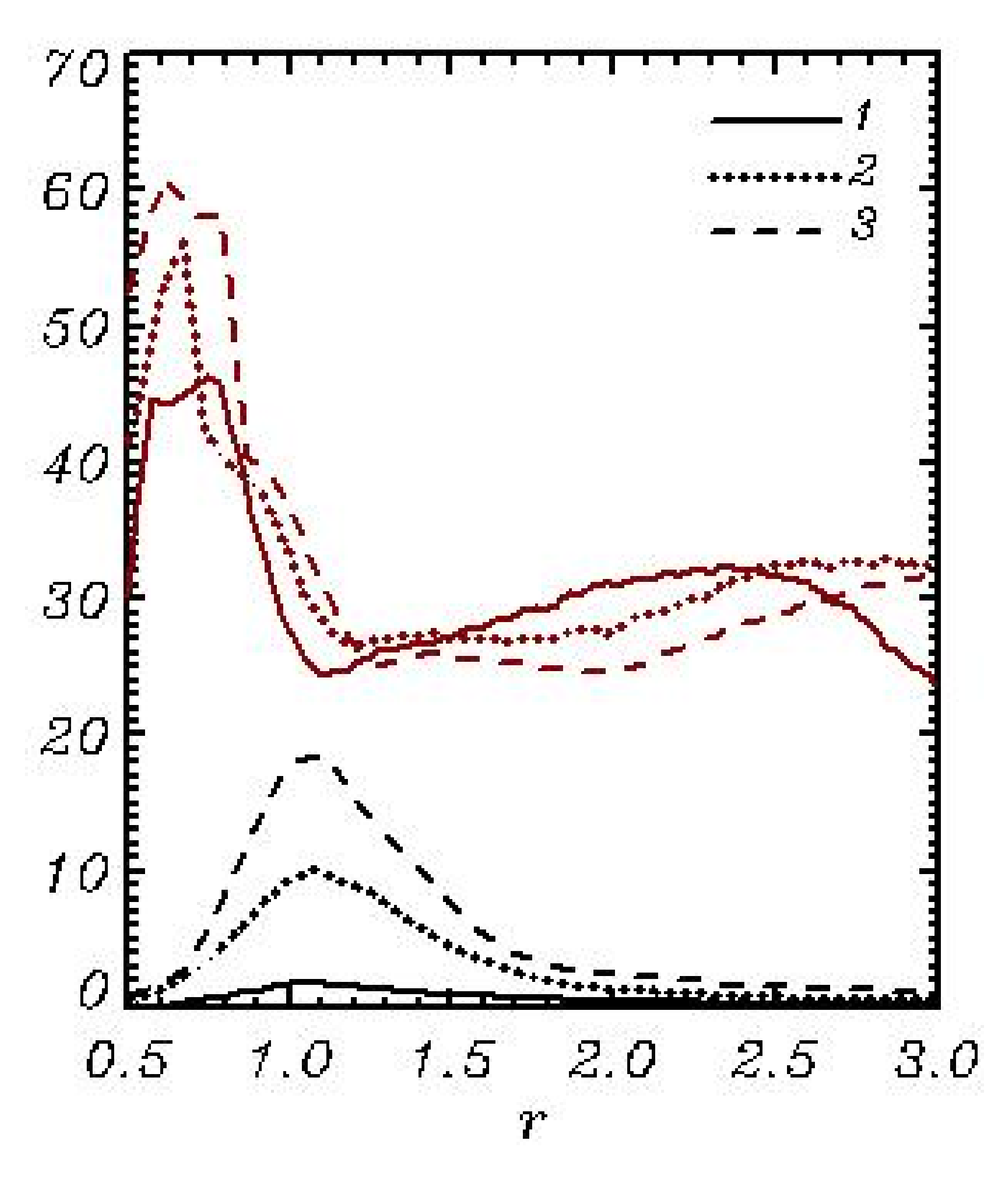
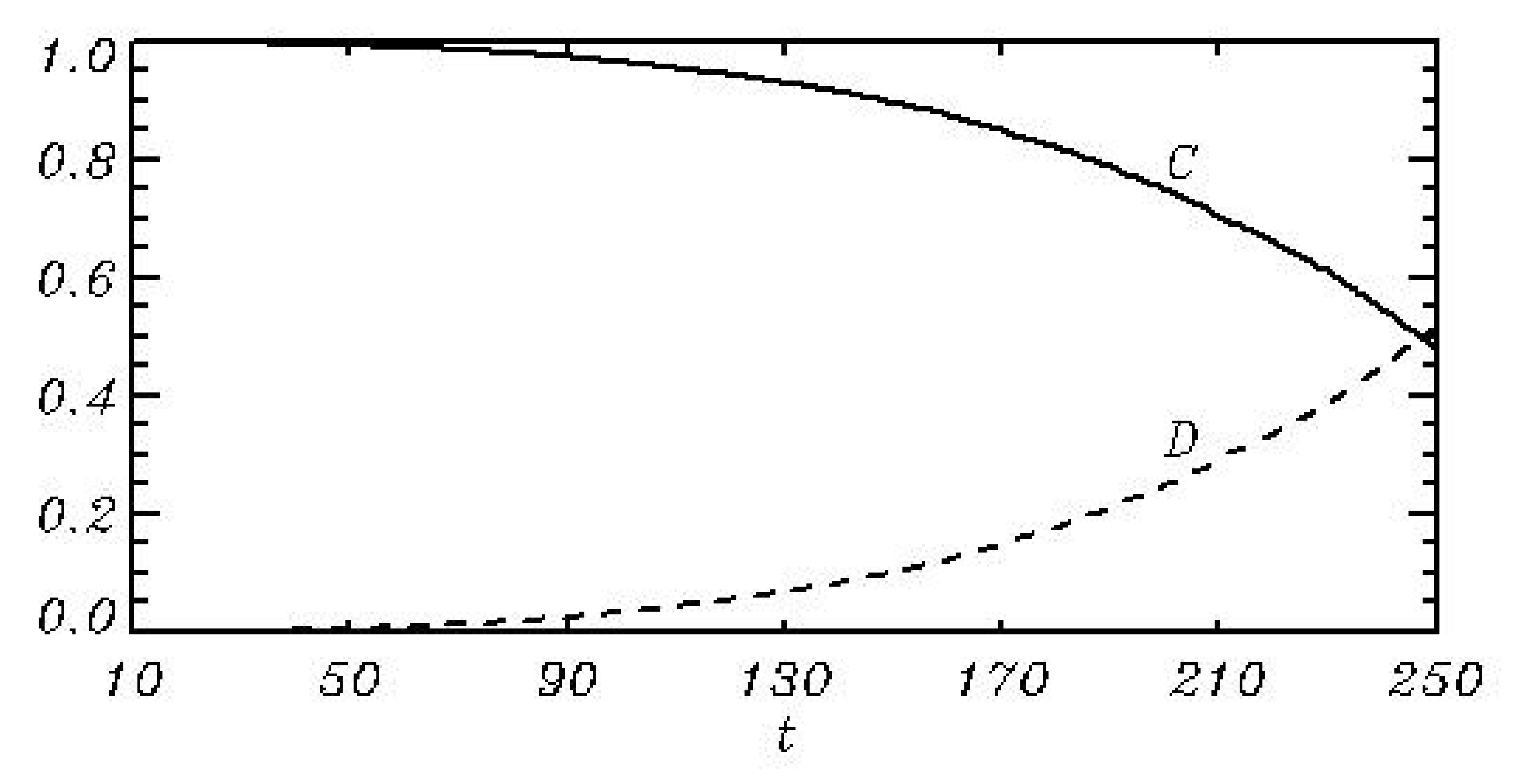
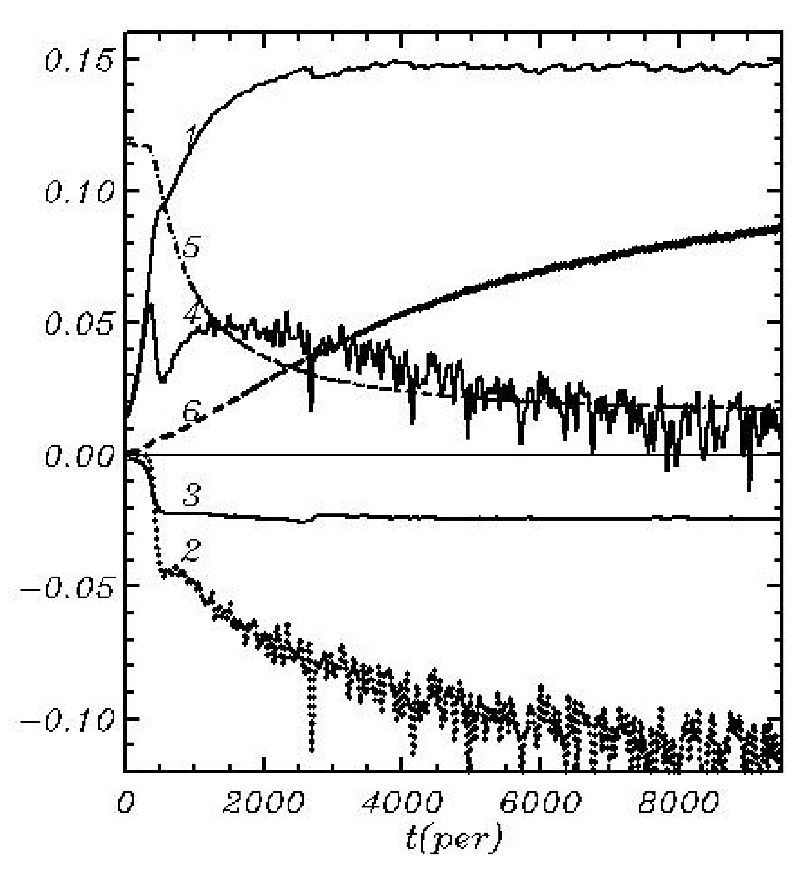
An evolution of integral characteristics as a function of time $t$ (expressed in the number of peak wave period $t_p=2\pi {\left({\mathrm{k}}_p\right)}^{-1/2}$ in the initial conditions) is given in Figure 7. The fastest change of all the characteristics occurs in the first $400t_p$ until the moment when the breaking dissipation $\overline{D_b}$ (curve 2) starts to develop. The input energy $\overline{I}$ (curve 1) remains nearly constant starting from $t=1000$. The total balance $\overline{I}+\overline{D_b}+\overline{D_t}$ (curve 4) gradually decreases but it does not turn into zero, and the total energy $\overline{\overline{E}}$ (curve 4) continues to grow. Curve (5) describes an evolution of the spectrum-weighted wave number $k_s$:

$$k_s={\left(\frac{{\displaystyle \int kSdkdl}}{{\displaystyle \int Sdkdl}}\right)}^{1/2}$$

(44)

It is a more convenient characteristic of the position of the spectrum because it changes in time smoothly. Over the time of integration, $k_s$ decreases from the value $k_s=120$ to $k_s=20$.

The nonlinear transformation of spectrum described by the right hand-sides of Equations (34) and (35) always produces the output of energy outside the computational domain in Fourier space. This process can be treated as dissipation. In our opinion, to keep the whole process under control, it is reasonable to maintain the total energy in the adiabatic part of the problem, governed by the initial Equations (4)–(6) with no input energy and dissipation. It can be performed by correction of all Fourier coefficients for the potential $f_{k,l}$ and elevation $h_{k,l}$:

$$f_{k,l}^{\prime }=\lambda f_{k,l}^{\prime },\hspace{1em}{h}_{k,l}^{\prime }=\lambda h_{k,l}^{\prime },$$

(45)

where a coefficient $\lambda$ is calculated by the formula

$$\lambda = {\left(E\left(f,h\right)/E\left(f^{\prime },h^{\prime }\right)\right)}^{1/2},$$

(46)

where $E$ is full energy calculated by a set of the coefficients $\left(f,h\right)$ before a time step and by $\left(f^{\prime },h^{\prime }\right)$—after a time step. The correction (45) and (46) is performed at each time step before calculating and adding the input and dissipation terms. A typical value of the coefficient $\lambda$ is $1\pm {10}^{-6}$. It is important that the correction (45) and (46) eliminates not only the loss of energy due to energy outflow from the computational domain but also due to the errors of approximations. A typical value of integral dissipation of this type was by around 2 decimal orders smaller than other energy transformation effects. Finally, the integral effect of nonlinear interactions was equal to zero (a thin straight line in Figure 8).

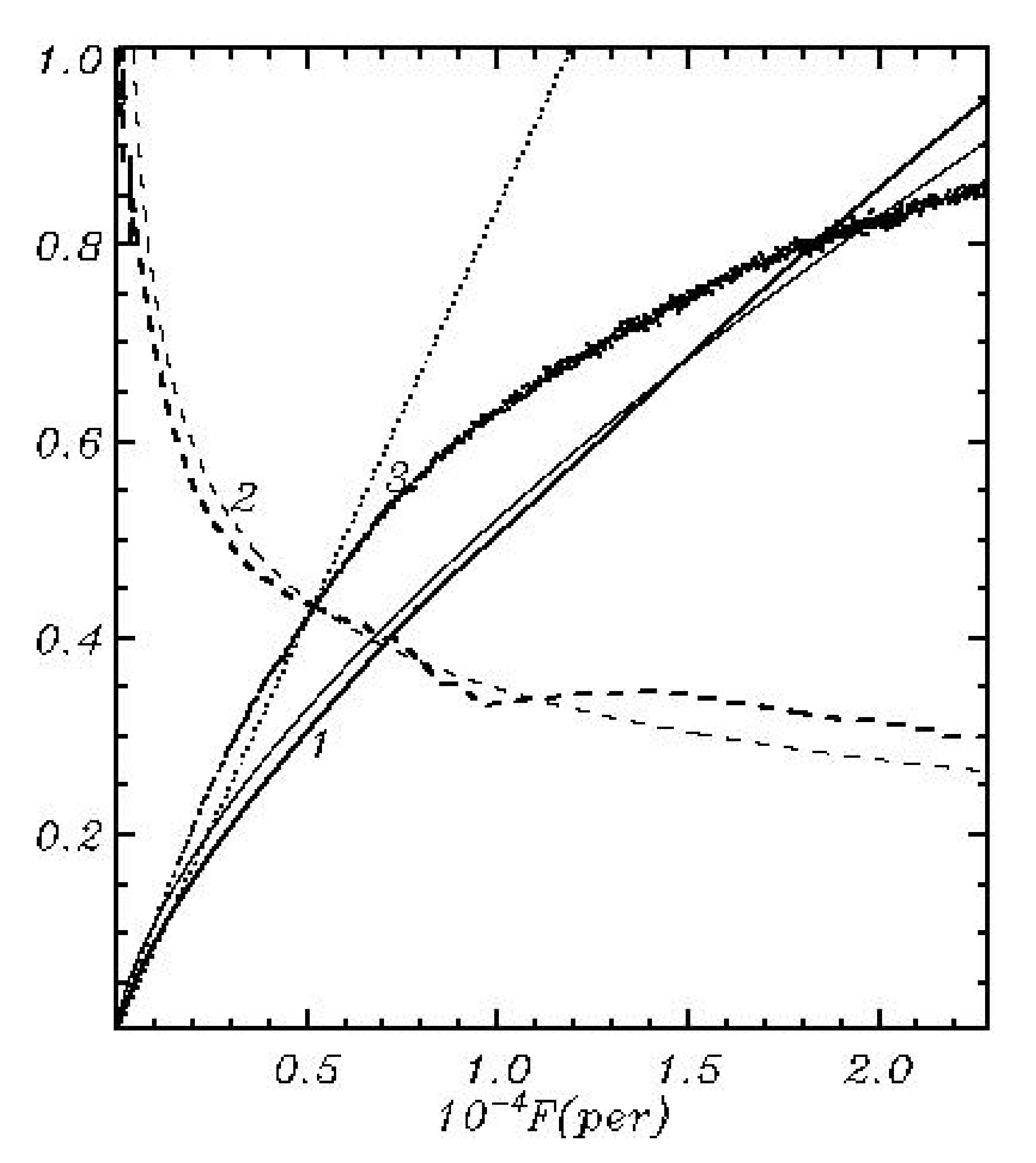
Additional integral characteristics are shown in Figure 8 where the computed values as a function of fetch $F.$ are compared with the same values calculated with a use of JONSWAP approximation [12]. Since the periodic variables are used, there is no other alternative but to assume that the fetch is a distance passed by a peak of the wave spectrum:

$$F(t) ={\displaystyle {\int }_0^t{c}_{p}dt}$$

(47)

The dependence of $F$ on $t$ can be obtained with a use of JONSWAP approximations:

$$F=3.34·{10}^{-3}{t}^{3/2}$$

(48)

The dependences (47) calculated by HWM and Eqauation (48) are shown in Figure 8 by thick and thin curves, respectively. As seen, these curves are quite close to each other. The dependence of peak frequency (defined as the frequency in a maximum of wave spectrum) is shown by curves 2. A dashed thick curve is calculated with the HWM model, and a thin curve corresponds to the dependence following from JONSWAP approximation:

$${\omega }_p=29.8F^{-1/3}$$

(49)

Opposite to Equation (44), the frequency ${\omega }_p$ is a point value. Due to the irregularity of the 2D wave spectrum, the peak frequency changes in time not monotonically but in jumps, and sometimes ${\omega }_p$ even moves back, i.e., to higher wave numbers. This is why the dependence $\omega \left(F\right)$ looks distorted. In Figure 8 this curve is smoothed. However, an agreement with the experimental dependence is quite obvious. The JONSWAP approximation of dependence of energy $E_p$ on fetch F is linear:

$$E_p=1.34·{10}^{-7}F$$

(50)

This dependence is shown in Figure 8 by a dotted line 3, whereas the dependence calculated by EWM is shown by thick dots. Those dependences agree with each other only at early stages of wave development. Evidently, an approximation (50) cannot be correct for a long fetch because it does not take into account the saturation of the spectrum. The more reasonable form is:

$$E_p=f\left({\mathsf{\Omega }}_p\right)F,$$

(51)

where $f$ is a function of the inverse wave age ${\mathsf{\Omega }}_p=U/c_p$ ($U$ is wind velocity).

In general, the results presented in Figure 7 and Figure 8 prove that an evolution of integral characteristics is reproduced satisfactorily.

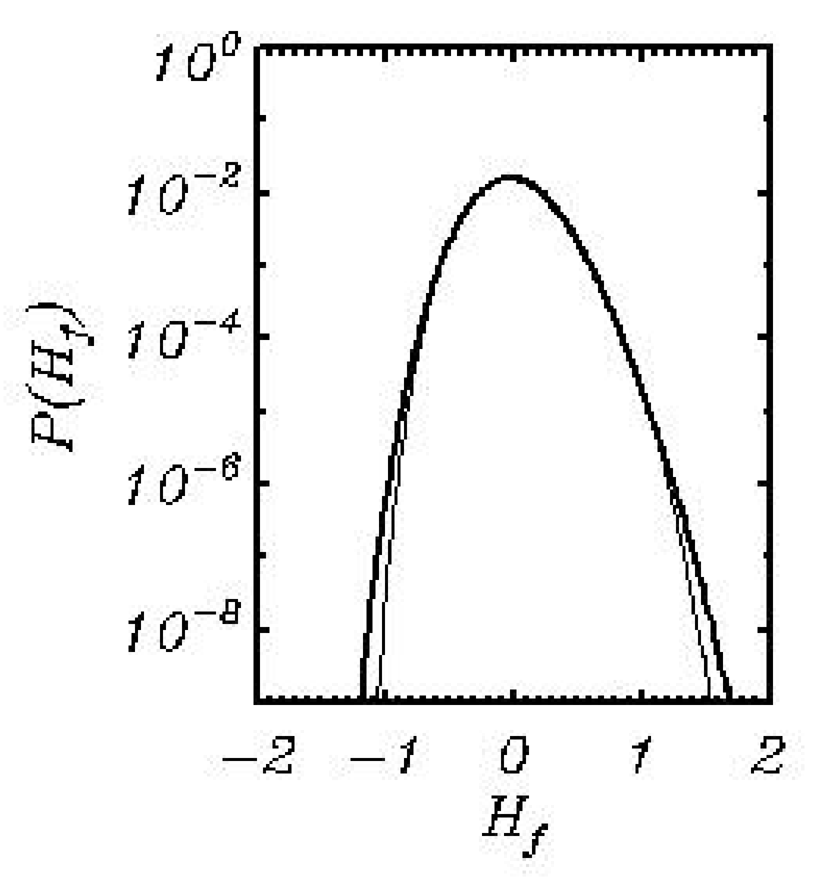
The HWM also reproduces well the probability of the nondimensional surface elevation ${\eta }_n=\eta /H_s$. The height of large waves predicted by HWM is somewhat bigger than that predicted by FWM [9] due to a larger total steepness of wave field and because the integration time was much longer. It is interesting to note that normalization of surface elevation by the significant wave height is so efficient that the probability distribution for the nondimensional surface elevation $P({\eta }_n)$ turns out to be nearly universal, i.e., it does not depend on wave energy and just slightly depends on total wave steepness. 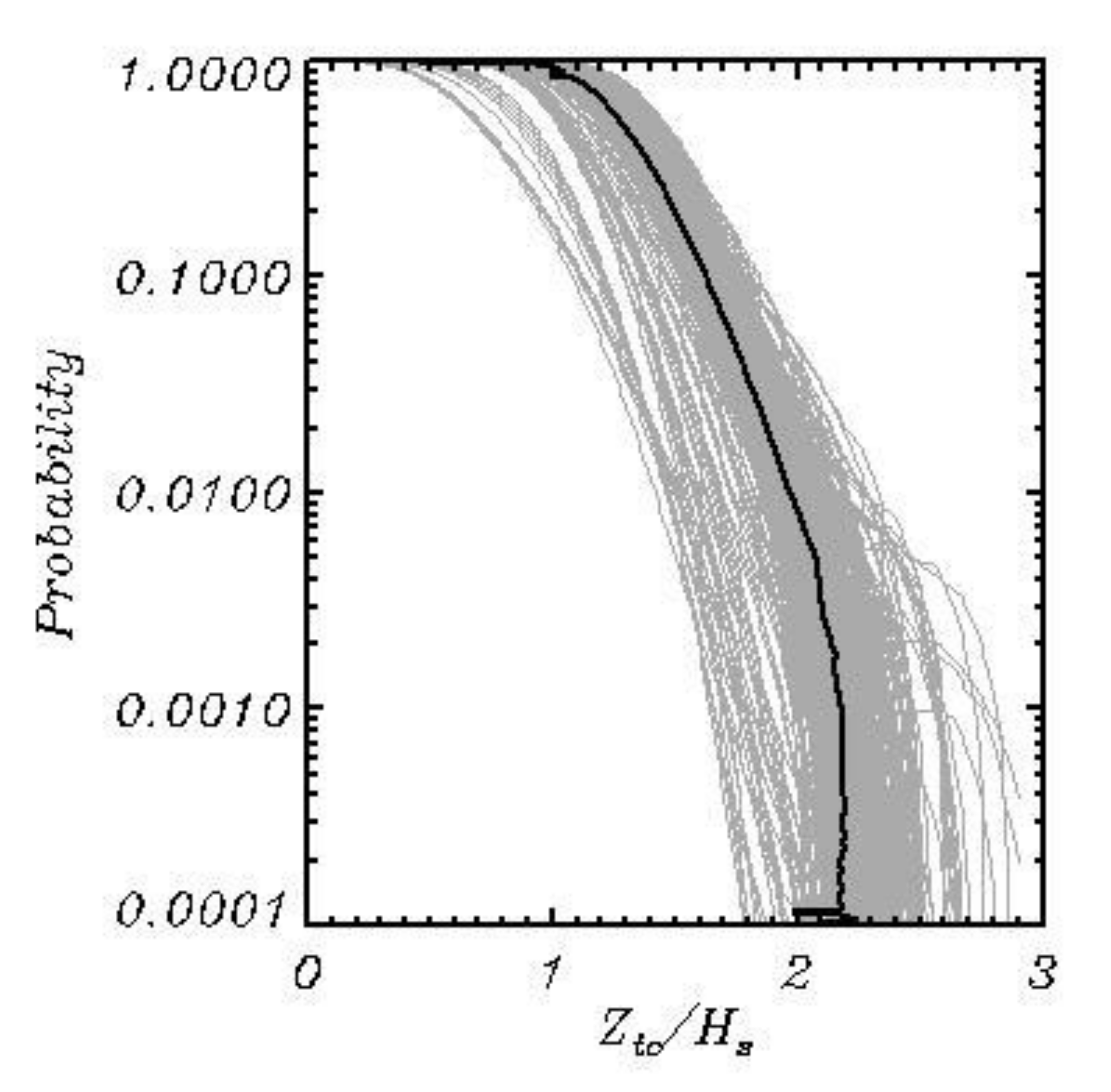Curves in Figure 9 are calculated over $3.1·{10}^8$ points; hence, it is not surprising that they are very smooth. In reality, the statistics of surface elevation shows very large scatter. The probability of the trough-to-crest height was calculated by a method of moving windows (see [13,14]). Each grey curve in Figure 10 is calculated over individual wave field containing 524.288 points. The total number of curves is 594. As seen, the probability for different wave fields variates in a broad range: many of them do not contain ‘freak’ waves with the height of ${\eta }_{tc}>2$ at all, whereas in many cases their height can exceed such a high value as ${\eta }_{tc}=2.5$ and even reach a value ${\eta }_{tc}=3$. This is why prediction of extreme waves for practical purposes is senseless with no indication of confidence intervals or distribution of probability for each value of ${\eta }_{tc}$.

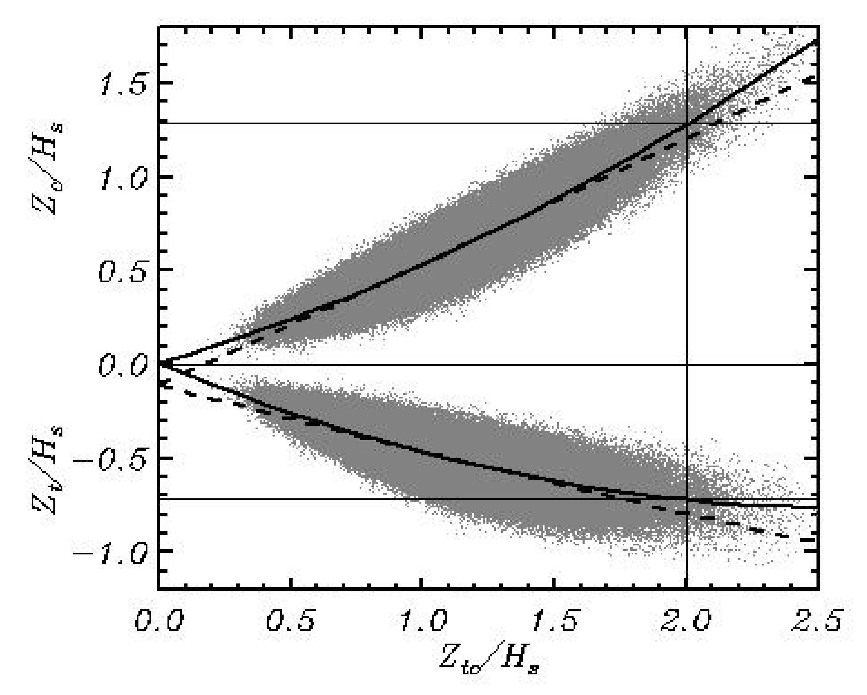
Figure 11 demonstrates statistical characteristics of positive and negative elevations as a function of the trough-to-crest height. As seen, the crest height $Z_c$ grows with the increase in total height $Z_{tc}$ faster than the trough depth, which can be explained by nonlinearity of the process. Figure 11 shows that on the average the trough-to-crest height $Z_{tc}/H_s=2$ corresponds to the crest height $Z_c/H_s=1.3$ and the trough depth $Z_t=0.7$. The dependences between those characteristics can be approximated by the formulas:

$$\begin{array}{l}{\tilde{Z}}_c=0.006+0.4162{\tilde{Z}}_{tc}+0.111{\tilde{Z}}_{tc}^2\\ {\tilde{Z}}_t=0.006-0.5838{\tilde{Z}}_{tc}+0.111{\tilde{Z}}_{tc}^2\end{array}$$

(52)

where tilde denotes normalization by the significant wave height $H_s$. Note that the first and third coefficients in approximation (52) coincide, which proves high quality of the ensemble. A dashed curve corresponds to the same data obtained with FWM [10]. The difference between the new and old data is growing for large values of ${\tilde{Z}}_c$. The old data contain 41.677 points, whereas a new array contains 1.264.441 points.

In a linear wave field (i.e., superposition of linear modes with random phases), the probabilities of crest height and trough depths are identical, but the probability of the trough-to-crest height is close to that for the nonlinear waves in a wave field with the same energy. This fact reliably proved with extensive calculations using the accurate two-dimensional and three-dimensional models [13,14,15], has not been explained yet. This fact seems to be directly related to the physics of extreme waves. The nonlinearity manifests itself in vertical asymmetry of waves, but not in the probability of full height.

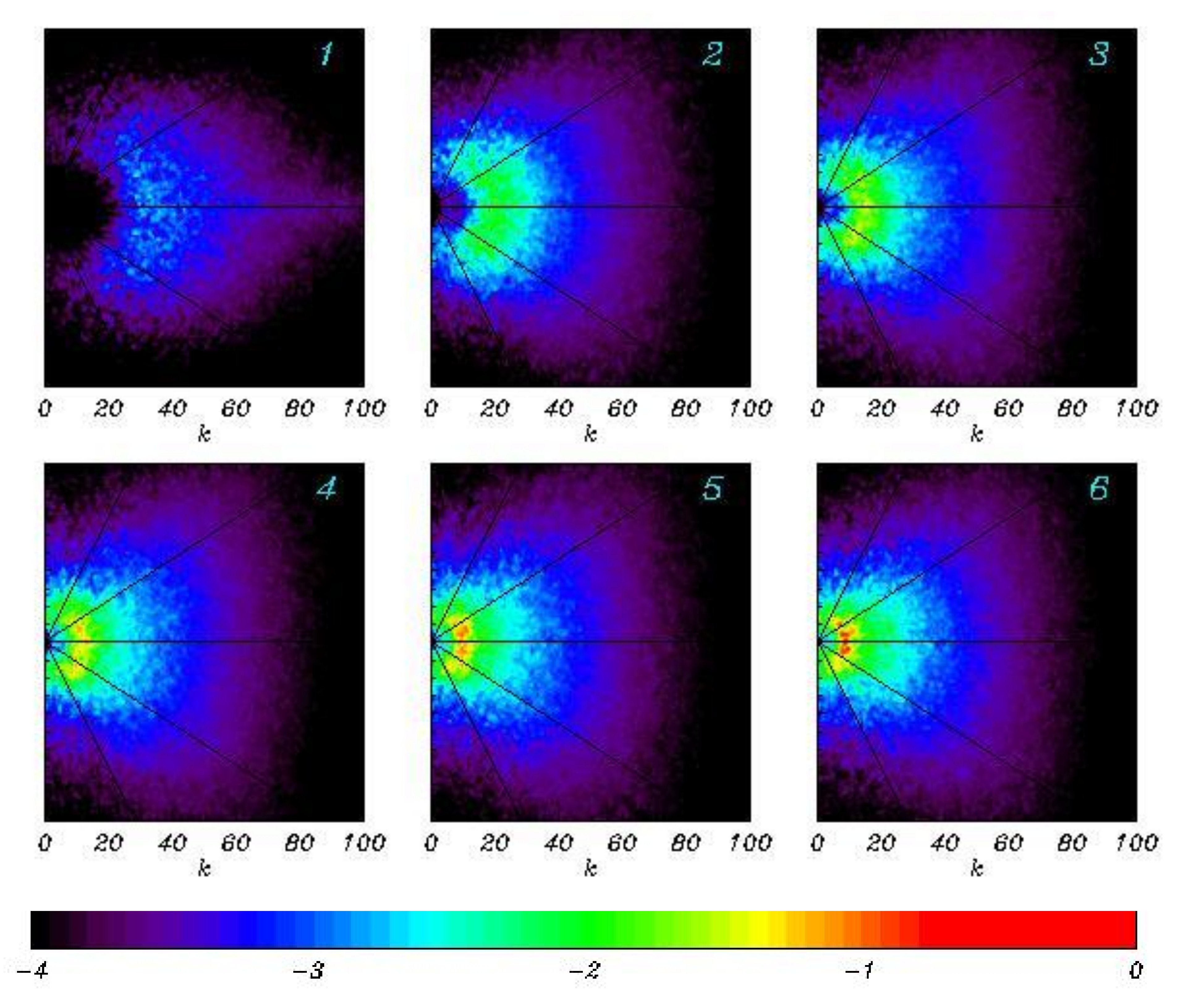
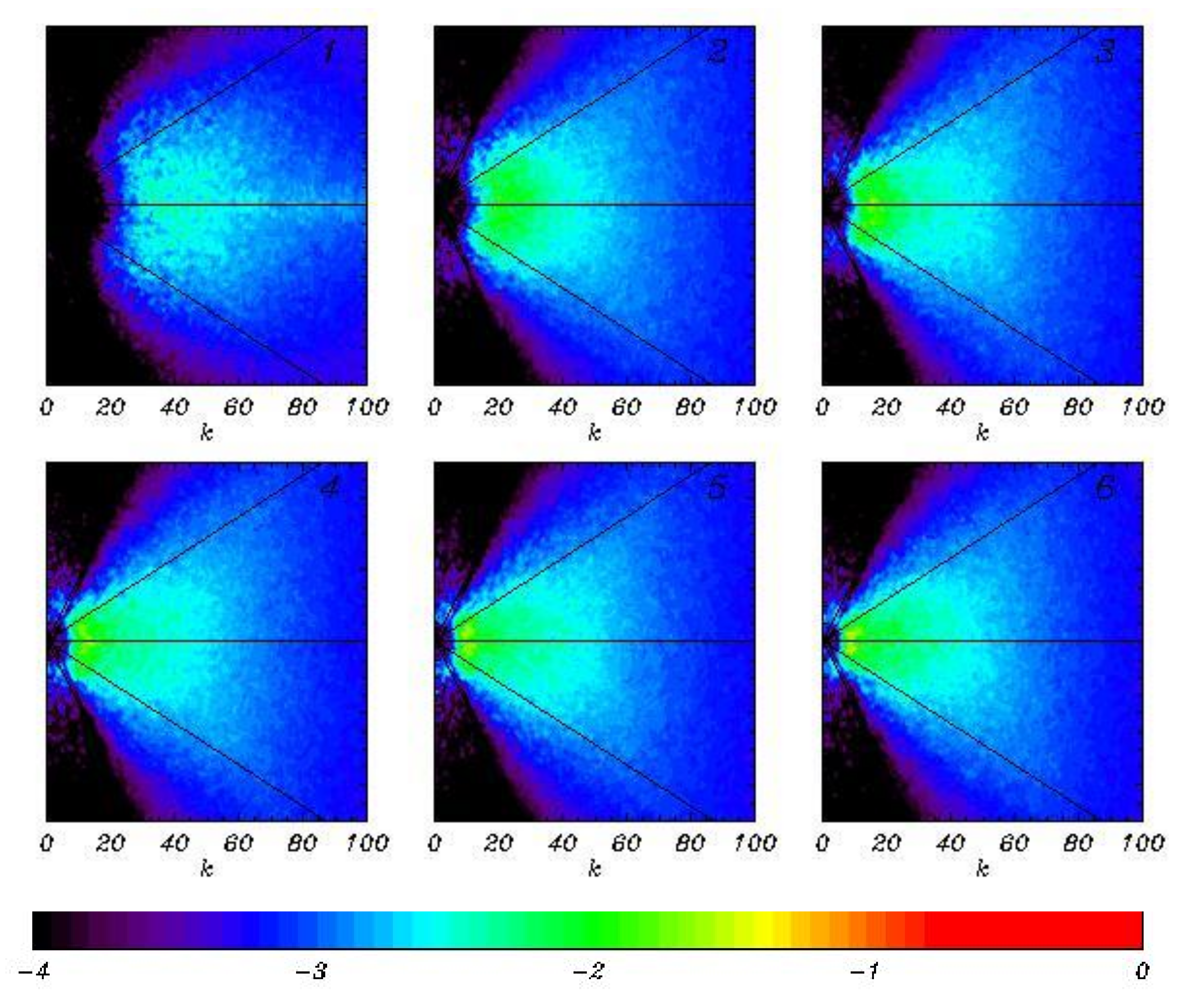
The next three figures show the 2D spectra obtained by averaging over six consecutive periods of length $t=1000$ (about 1600 initial peak period). Each spectrum is calculated by averaging 100 spectra transformed into the polar coordinates $\left(\theta ,\mathrm{k}\right)$. The surface elevation spectra $S\left(\theta ,\mathrm{k}\right)$ are given in Figure 12. The colors correspond to different values of ${\log }_{10}\left(S/S_m\right)$ where $S_m$ is a maximum of the last of the six spectra. A minimum value (black color) corresponds to the values less than ${10}^{-4}{S}_m$. It is seen that the spectrum grows and approaches the point $\mathrm{k}=0$. Despite the severe averaging, the spectra look highly irregular. They contain multiple peaks and holes (well seen in panels 5 and 6). The discussion of this effect is given in [7,13].

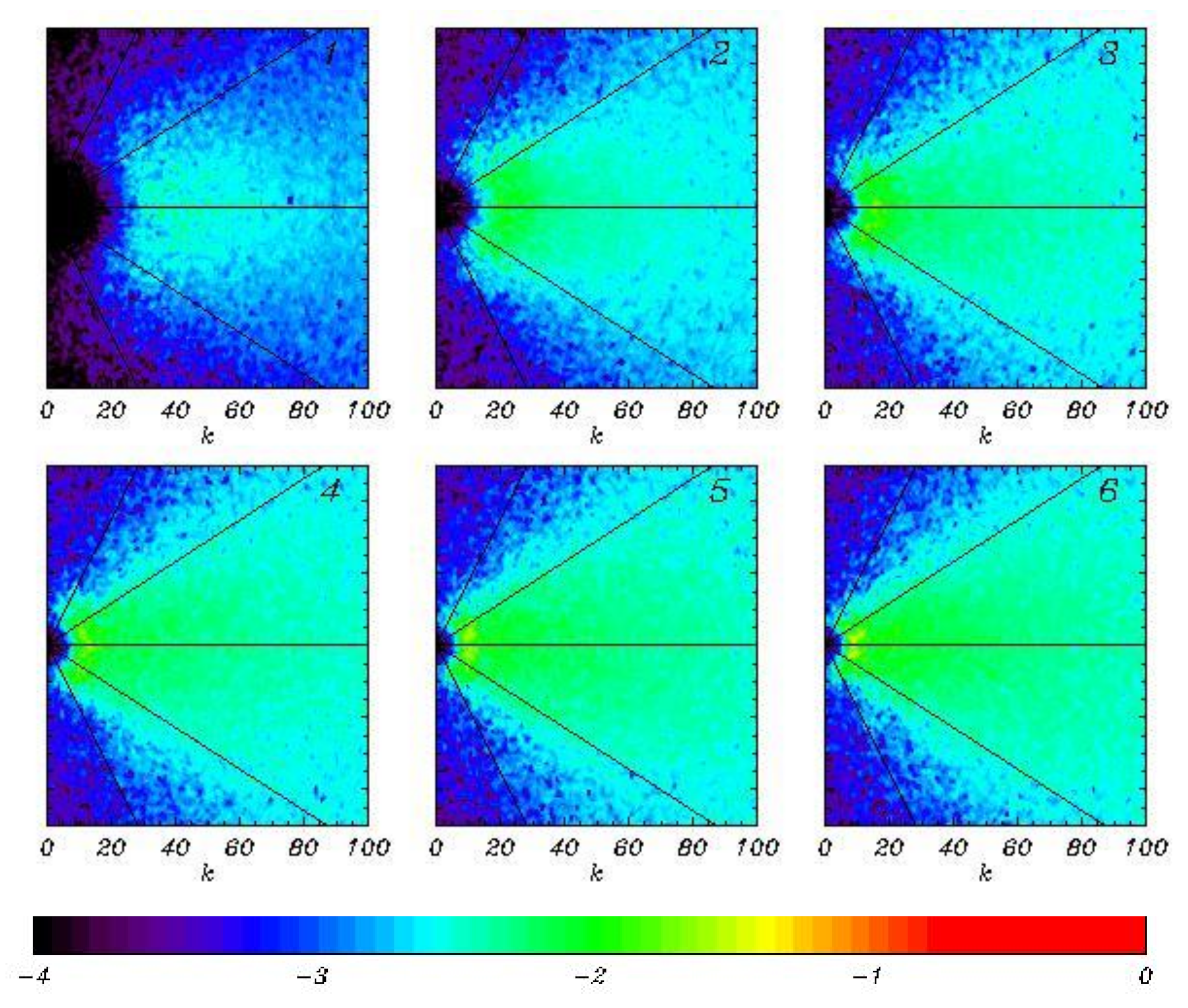
The spectra of the energy input shown in Figure 13 calculated similar to wave spectrum are much wider than the wave spectrum, because the input of energy decreases with growth of wave number slower than the wave spectrum. It happens because $\beta$-function (see [16]) depends on wave number quadratically. For large fetches the areas of negative wind input in low wave numbers (i.e., a flux of energy from fast wave modes to wind) usually arise, but it cannot be shown in the given figures.

The spectra of total dissipation rate equal to the sum of breaking and tail dissipation, are shown in Figure 14. A maximum of dissipation always falls on a maximum of wave spectrum. However, dissipation, as well as the input energy, occurs everywhere including the spectral tail. Here, as in all our previous calculations, we did not reproduce an adiabatic regime at the spectral tail, which excludes any possibility to draw analogy to Kolmogorov’s spectrum. The attenuation of energy in the spectral tail depends on a shape of entire spectrum, as well as on wind velocity, wave age and other factors.

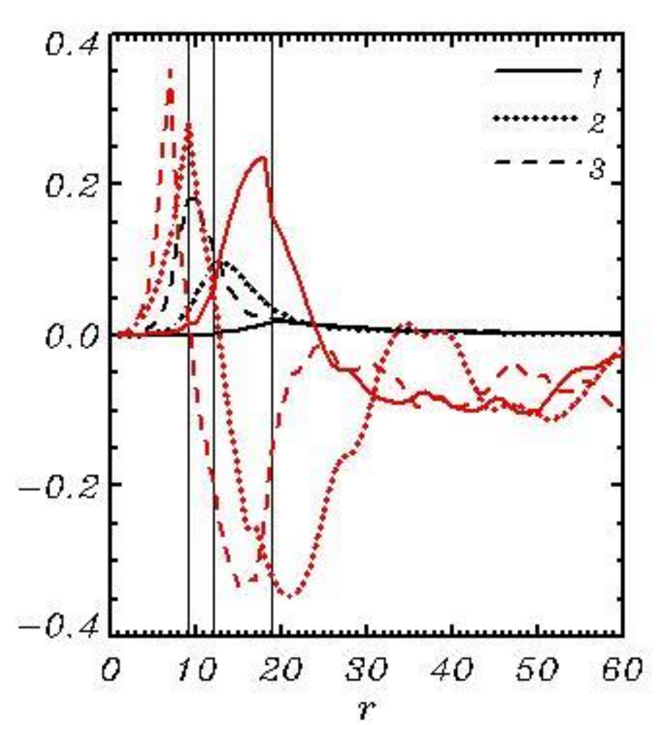
The process of downshifting is well seen in Figure 15 where the evolution of 1D wave spectra (black curves) and the spectra of the nonlinear transformation rate (red curves) in the vicinity of a peak averaged over three consequent periods, each of $t=2000$ length, are given. All the spectra are calculated over 198 records of the two-dimensional spectra transformed into the polar coordinates, summated over angles and represented as a function of radius $r=\mathrm{k}$. The locations of a wave spectrum maximum are indicated by thin vertical lines. Note that the analysis of the spectra for a nonlinear transformation rate is not simple, because the dispersion of reversible exchanges of energy between the modes is much higher than the rate of residual irreversible interaction. The accuracy of calculations grows with increase in spectral resolution. The recently launched calculations with HWF using spectral resolution of $1027\times 1027$ modes gave the averaged spectral distribution much smoother than that in Figure 15. In general, the spectra in Figure 15 agree with the known regularities: the energy from a right slope of wave spectrum is transferred to the left slope, i.e., to longer waves. It qualitatively confirms Hasselmann’s theory [17] considering the four-wave interactions. Opposite to that theory, actual interactions occur between all the spectral modes within the scope of the Fourier transform method. Unfortunately, the quantitative comparison with the theory is impossible since neither of the codes for calculation of Hasselmann integral can operate with such a high number of modes as used in phase-resolving models.

Most of the energy coming from wind to waves dissipates because of wave breaking. A currently used parameterization method for wave breaking is based on a diffusion algorithm with a variable coefficient of diffusion applied to both the elevation and surface velocity potential. The breaking occurs when Laplacian of elevation $\Delta ={\eta }_{\xi \xi }+{\eta }_{\vartheta \vartheta }$ becomes smaller than the negative value ${\Delta }_c$ (in the current model ${\Delta }_c$ = −80). A diffusion coefficient $B$ is defined as follows:

$$B=\left\{\begin{array}{cc}{C}_b{\left(\Delta x^2\Delta \right)}^2& \Delta <{\Delta }_c\\ 0& \Delta \ge {\Delta }_c\end{array}\right.,$$

(53)

where $\Delta x$ is a horizontal step, and $C_s=0.02$ is a coefficient. The parameters ${\Delta }_c$ and $C_b$ are selected with consideration of a rate of growth of total energy. It is remarkable that the integral rate of breaking dissipation is not too sensitive to the choice of parameters because the effects of frequency of breaking (regulated by ${\Delta }_c$) compensate for the intensity of breaking (depending on $C_b$). The rate of breaking seems to depend mostly on a rate of the energy input: most of the energy should be removed to maintain the numerical stability in the model, i.e., to prevent appearance of too sharp waves. Obviously, in a real wave field similar effects occur: dissipation absorbs extra energy obtained from the wind. Though a suggested algorithm seems very simple, the scheme performs all that is required.

Note that some part of the released horizontal momentum and energy should be transferred to horizontal motion (current). This effect cannot be taken into account in a potential model. The energy released after breaking is partially dissipated and partially distributed in space and between the wave modes, thus additionally contributing to the nonlinear interactions. The effects of breaking are presented in Figure 16 where the number of breaking cases (% of the total number of knots) and the integral rate of energy loss at each time step are presented. As seen, both characteristics grow in time with the tendency for stabilization by the end of a run.

At an early stage of the work on parameterization of breaking the attempts were made to construct a scheme based on the geometrical and mechanical consideration with direct calculations of the stability criterion, a detaching volume of water and the possible consequences. Finally, we came to the conclusion that such a scheme would never work properly or be sufficiently robust to be used at millions of grid point and time steps. It is more reliable to adhere to the standard methods adopted in the geophysical fluid mechanics.

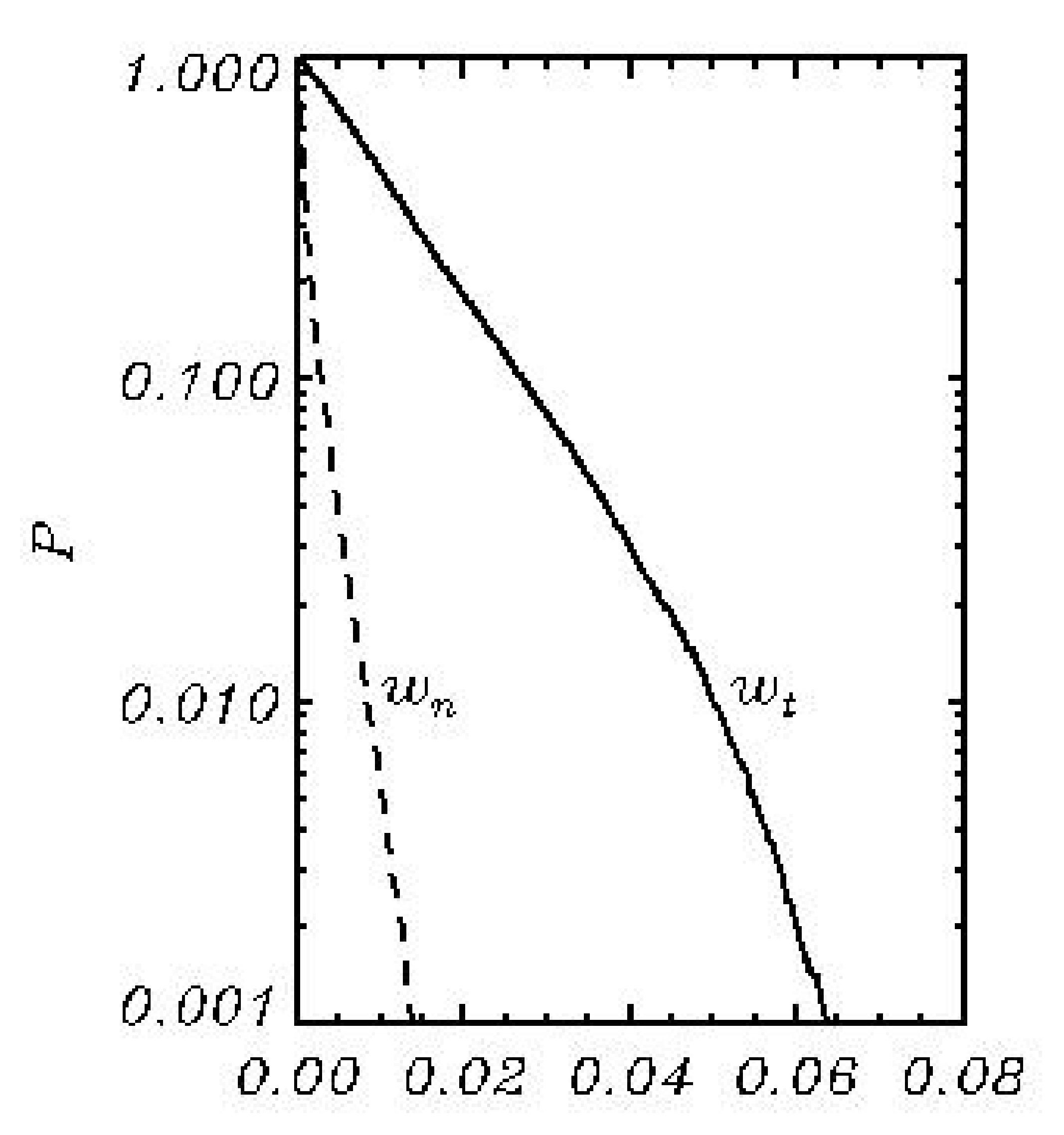
The width of spectrum can be characterized by a function $\mathsf{\Psi }\left(\omega /{\omega }_p\right)$ (see [18,19]).

$$\mathsf{\Psi }=\frac{{\displaystyle \int S\left(\omega ,\psi \right)\left|\psi \right|}d\omega d\psi }{{\displaystyle \int S\left(\omega ,\psi \right)}d\omega d\psi }$$

(54)

where integrals have taken over the domain $\left\{\left(0<\omega <{\omega }_c\right),\left(-\pi /2<\psi <\pi /2\right)\right\}$. The wave spectra as the functions of frequency $\omega$ normalized by peak frequency ${\omega }_p$ for the same three periods shown in Figure 15 are given. As seen, the $\mathsf{\Psi }$ curves corresponding to different wave ages are close to each other. All of them have a sharp maximum at the frequencies below the spectral peak, as well as a well-pronounced minimum in the spectral peak and a relatively slow growth above the spectral peak. The decrease in $\mathsf{\Psi }$ at high frequencies is probably caused by the high-frequency dumping. The angle distribution was investigated in [18,19]. The approximations of $\mathsf{\Psi }\left(\omega /{\omega }_p\right)$ from the different sources collected in [20] show considerable scatter, but the general features are quite similar to those shown in Figure 17.

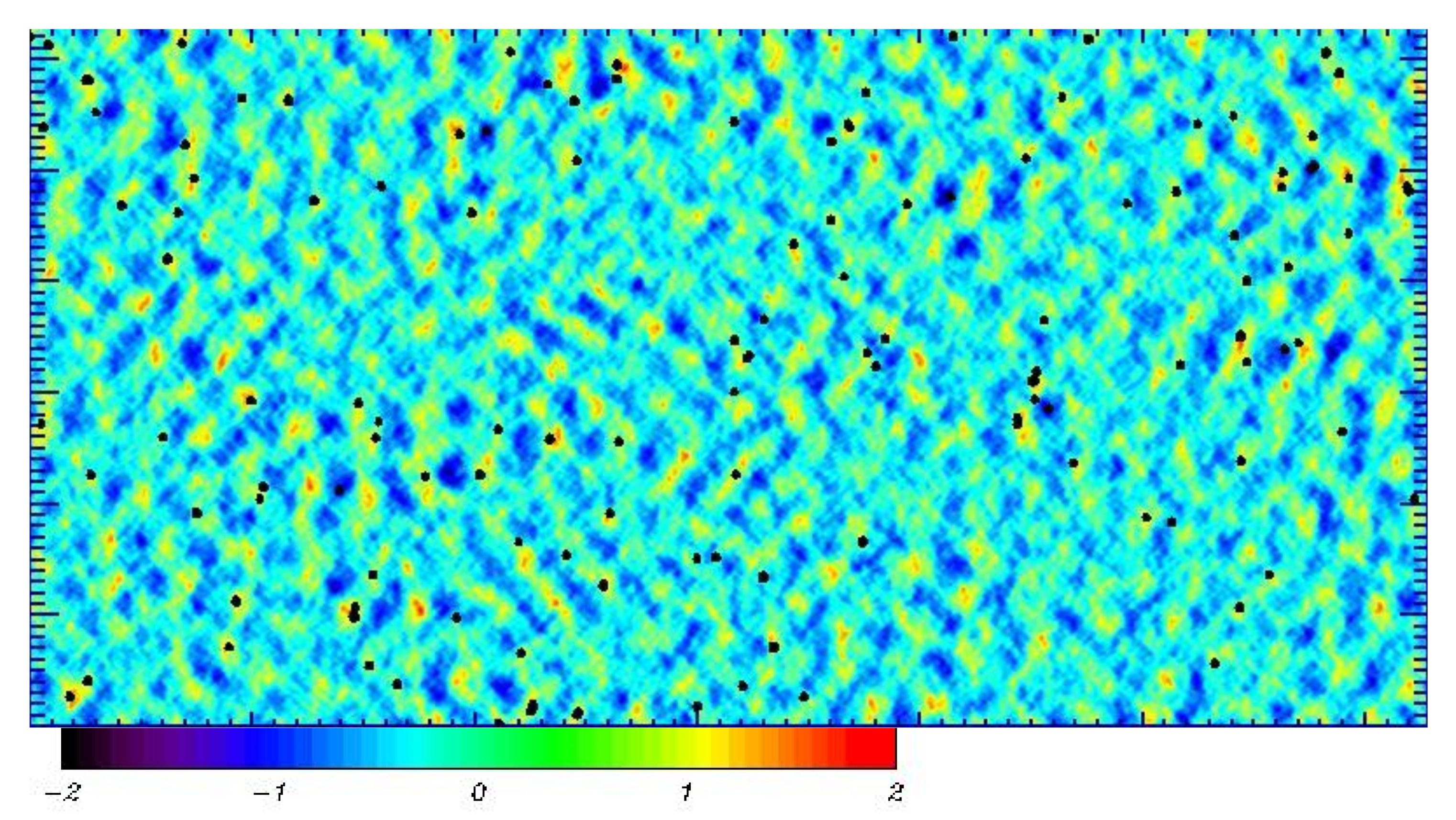
An example of a simulated elevation field $\eta$ normalized by the significant wave height $H_s$ is given in Figure 18. In the initial conditions, small unidirected waves at inverse wave age $U/c_p$ were assigned. In Figure 18 we can see a developed three-dimensional field with the energy by two decimal orders higher than that in the initial conditions, and the broad angle distribution. Black dots mark the points where breaking occurs at a given time step.

4. Conclusions

The three-dimensional modeling of surface waves based on full nonlinear equations is a powerful tool for the investigation of wave processes, development of the parameterization schemes for the phase-resolving and spectral models and direct simulation of wave regimes in small basins. This type of modeling is rapidly developing. However, all approaches have a common limitation, i.e., low computational efficiency. Working with such models, even with modest resolution, turns into an endless waiting of the results. This property of the models slows down their improvement, in particular, development of the parameterization schemes for physical processes, since such work requires multiple repetitions of the runs. Such schemes significantly depend on resolution of a model, which limits the possibility of the research with low-resolution models.

The current paper continues to develop a new approach to the phase-resolving modeling of two-dimensional periodic wave fields at infinite depth. The basic concept of the scheme follows from presentation of the velocity potential as a sum of the linear and nonlinear components suggested in [7]. The solution for a linear component is known; hence, a nonlinear component should be calculated through Poisson equation with a zero-boundary condition on the surface. It was observed in [10] that such approach offers a new way to simplify the calculation by considering of 2D Poisson equation on the surface. The equation that can be treated as additional exact surface condition contains both the first ${\phi }_{\zeta }$ and second ${\phi }_{\zeta \zeta }$ vertical derivatives of the potential. Thus, the system of equations remains unclosed. It was empirically discovered that these variables are closely connected to each other. The linear dependence between ${\phi }_{\zeta }$ and ${\phi }_{\zeta \zeta }$ was checked in [10]. It was shown that the use of such hypotheses leads to formulation of a closed system of equations.

In this paper, the above approach was improved by introducing a more flexible dependence of a ratio ${\phi }_{\zeta }/{\phi }_{\zeta \zeta }$ on the nondimensional integral parameters of the wave field. The comparison of full vertical velocity $w={\phi }_{\zeta }$ calculated using a new method, with that calculated by FWM, shows good agreement (Figure 5). The point-to-point comparison of runs with HWM and FWM starting from the identical initial conditions proves that the solutions agree over thousands of time steps (Figure 6). A long high-resolution run with HWM revealed that a simplified model produces the statistical results similar to those obtained with FWM [9]. The main advantage of the new approach is high computational efficiency. The ratio of time spent for calculation with identical FWM and HWM variated in the range of 50–100. This ratio depends on complexity of parameterization of physics and volume/frequency of the processed and recorded information. Some acceleration can be reached by replacing a Runge–Kutta time integration scheme with a high accuracy one-step scheme.

The model suggested is not mathematically precise since it is based on the empirical (in computational sense) connection between the local variables, i.e., vertical velocity and its vertical derivative. The fact that those variables are connected by an equation containing horizontal derivatives indicates that the local connection cannot be exact. To discuss this problem, it is necessary to answer a general question: what does the concept of precision mean?

It should be noted that surface waves are often investigated on the basis of different simplified equations such as a linearized Navier–Stokes equation, Korteweg de Vrie equation, a linear and nonlinear Schrödinger (NLS) equation and others. No one actually knows which real properties of sea waves are omitted in those models. In some simplified approaches (e.g., in the models based on a nonlinear Schrödinger equation (see [21]), the instability of high waves is missing; hence, the amplitudes of simulated waves can be unrealistically large. In reality, an excessive growth of waves is prevented due to the energy focusing and wave-breaking instability. The models based on the full potential equations predict the probability distribution for large waves quite satisfactorily. The main obstacle to a widespread use of the models based on complete equations is their low computational efficiency. An approach suggested here eliminates this obstacle by excluding reproduction of a three-dimensional flow structure. However, nothing prevents us from using a combined model with the on-demand calculations of a three-dimensional field of the velocity potential. A simplified model gives almost the same statistical results as a full model. Essentially, the difference between the statistical results given by 3D and 2D models are similar to those obtained with a 3D model initiated at different sets of random phases. It is easy to see that the equations suggested above are completely similar to the full equations, with one exception, i.e., a small non-linear correction to the total vertical velocity is calculated not from a 3D Poisson Equation (12) but from a simple 2D Equation (17). It can be added that a simplified model has a much simpler structure than FWM and is easily programmed. It is known that in most cases the data on 3D velocity potential are not required, but, if necessary, they can be easily obtained periodically in a process of model run or by the post-processing using the restart records and the corresponding subroutines adopted from 3D FWM.

It is obvious that an approach developed here is not fully precise. For example, it cannot be applied for individual cases with a small number of modes, for example, for simulation of a steep Stokes wave, as it was demonstrated for FWM in [7,9]. The 2D model is intended for simulation of the statistically homogeneous multi-mode wave field.

To continue the discussion on the accuracy problem, it should be noted that the full 3D adiabatic model is also inaccurate, because it is suitable for relatively short time intervals only. Real waves receive energy from wind and dissipate. Currently, such processes are poorly studied because they are evidently more complicated than the wave movement itself. Therefore, neither of the models can be considered as fully adequate. Especially for the followers of high accuracy it should be added that the full potential equations are far from being accurate even for the waves with no input energy and breaking. Real waves develop in a flow with the velocity shift, and they exchange energy with vortex movements [22]. Therefore, they are better described by the Navier–Stokes equations. As a result, we obtain a variety of problems associated with the turbulence. It may turn out that the simplifications used in the construction of this model may be quite insignificant, as compared with other disadvantages.

Certainly, there are many ways to improve the model, first of all, for example, testing of alternative schemes for calculation of a nonlinear velocity component (Equations (31)–(33)). The attempts were made to construct the closure scheme for a surface Poisson equation in Fourier space. This way turned out to be unrealistic, since the local structure of the velocity potential depends not only on Fourier variables but also on a local full elevation.

The most evident advantage of a new model is the absence of calculation of the 3D structure of the velocity potential, which increases the speed of calculations by around two orders. This easily programmable model can be used to improve the physical components of the model and the long-term simulations of a multimode wave field. The model can be also used for acceleration of the calculations as a block of an exact 3D model (such as FWM). This coupling provides the possibility of runtime tuning of the parameters of the closure scheme for a surface Poisson equation.

The scope of practical applications of such model is quite wide. First of all, it should be used for building up of parametrization of physical processes in spectral and phase-resolving models. HWM, due to its high performance, can be used as a component of wave prediction models (such as WAM or WAVEWATCH) for interpretation of spectral information in terms of the phase-resolved wave field. A possible consecution of action is as follows: the spectra calculated in the spectral model in the selected areas are used for generation of the initial conditions in the wave number space; then the calculations up to the stationary statistical regime with HWM are performed; finally, the statistical characteristics of wave field including the probability distribution of wave height are calculated. The input and dissipation terms can be included in such simulation. Note that such approach allows calculating nonlinear interactions between all the modes based on full nonlinear equations. Such scheme can significantly extend the output of spectral modeling.

It is comparatively easy to transform the scheme into a finite-difference form and use the model for investigation of a wave regime in a specific geographical environment with variable boundary conditions. Note that a numerical scheme for this model is much closer to the local scheme than FWM, which makes convenient to carry out the parallel computations. An investigation of applicability of a developed approach for the waves above finite depth is underway.