A BEM-Based Model of a Horizontal Axis Tidal Turbine in the 3D Shallow Water Code SHYFEM

Abstract

We present a novel 3D implementation of a horizontal axis tidal turbine (HATT) in the shallow water hydrostatic code SHYFEM. The uniqueness of this work involves the blade element momentum (BEM) approach: the turbine is parameterized by applying momentum sink terms in the x and y momentum equations. In this way, the turbine performance is the result of both the flow conditions and the turbine’s geometric characteristics. For these reasons, the model is suitable for farm-layout studies, since it is able to predict the realistic behavior of every turbine in a farm, considering the surrounding flow field. Moreover, the use of a shallow water code, able to reproduce coastal morphology, bathymetry wind, and tide effects, allows for studying turbine farms in realistic environments.

1. Introduction

In recent years, the need for unbound power generation from fossil fuels has led to renewable resources. In this scenario, tidal energy is receiving more interest due to its predictable character and minimal visual impact. Many devices are able to exploit tidal energy, but only a few have reached a technology readiness level (TRL) suitable for in situ applications [1]. The most relevant category, in this sense, is represented by the horizontal axis tidal turbine (HATT), which benefits the wind energy field.

However, to date, there are no commercial examples of HATT farm applications. Moreover, we cannot take advantage of the wind energy field for concerning turbine farm evaluations, since the flow conditions are completely different. The tidal sites, suitable for energy exploitation, are often located in shallow water (with confinement, with respect to the vertical direction); the horizontal direction may be limited in channels, straits, inlets, and so on, where higher flow velocities are reached. Hence, there is a need to cover the knowledge gap in this field in order to optimize the layout and the operating conditions of the farms. Both in situ and laboratory experiments are very expensive and not exhaustive. On the one hand, the most common limitation of a laboratory-scale study is the impossibility to reproduce flow conditions of interest. For instance, it is not possible to reach Reynolds numbers in realistic operating conditions. In a wind tunnel, it is possible to reach a flow velocity of about 30 m/s to compensate for the physical model size, but in a flume, it is difficult to overcome 1.5–2 m/s. Moreover, blockage effects are often present, especially when experiments are used to analyze interactions between several devices. Furthermore, in a cluster of laboratory scales, the number of tested devices is limited. The following references are examples of experimental studies on hydrokinetic turbines: [2,3,4], where the number of tested devices increased from two to a maximum of four. On the other hand, the in situ studies with prototypes of proper sizes allow evaluating realistic flow conditions, but they are often limited to single devices. For these reasons, it is essential to develop tools that are able to perform farm simulations in order to help researchers plan and design the optimal farm layouts. Because of the site-dependent characters of the energy resources, it is necessary to reproduce realistic conditions for the simulations. To this end, shallow water marine codes, usually used for oceanographic purposes, are the most adequate instruments if properly adapted to tidal energy converters evaluations.

Many studies have dealt with tidal turbine farms performed using shallow water software, but most were 2D studies where the turbine was parameterized by an additional drag force [5,6,7,8,9]. This approximation is useful for saving time and making preliminary evaluations, but it completely neglects the three-dimensional effects, making the analysis incomplete. Some other works have used more precise 3D parameterizations with momentum sinks [10,11,12]. Both 2D and 3D models often make use of constant thrust coefficients, which are imposed to reproduce the turbine effect. In this way, constant behavior for all turbines in the arrays is adopted, without considering the interactions and mutual influences between devices. In [8,10], a variable thrust coefficient, depending on the rotor axial velocity, was adopted; however, such an accurate model is still unable to capture the effects of the mutual influences of devices. Indeed, it does not consider the flow effects due to acceleration corridors, which increase between devices. To our knowledge, there are no examples in the literature that make use of the blade element (BE) approach: in brief, the BE theory allows for evaluating the performance of the device by calculating the forces acting on the blades; the blade is made up of blade elements of infinitesimal radial thicknesses. This allows evaluating the behavior of the turbine considering the geometrical characteristics and the operating conditions. For instance, it is possible to evaluate the influence of changes in the rotational speed of each device in a farm in order to maximize the energy output. Since the aim of tidal farm optimization is to enhance power production, we found it necessary to develop a tool that is able to predict (in a more accurate way) the behavior of the farm and every device.

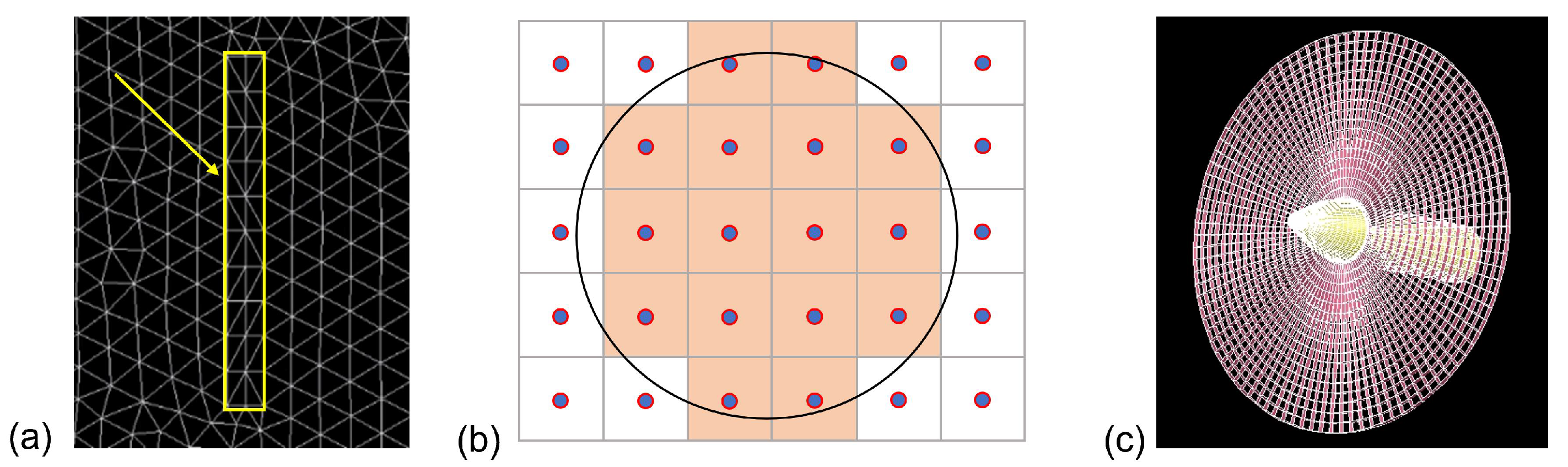
In the present paper, we used the SHYFEM open-source code developed at the CNR-ISMAR of Venice [13]. In order to obtain a highly precise turbine reproduction, we applied an approach based on the blade element momentum (BEM) theory using a high-resolution grid. The turbine was modeled by means of hundreds of grid elements. Other works used resolutions finer than those usually used for oceanographic purposes but were still coarse for accurate turbine parameterization. In [10], for instance, a 20 m diameter turbine is represented with a horizontal resolution of 20 m × 20 m and is identified with three vertical layers. These elements will allow one to make a thorough prediction of the turbine behavior for performance and wake development. The high-resolution grid also allows one to evaluate the effects of small geometrical or operational changes in a device.

This paper is structured as follows: in Section 2, we summarized the theoretical background of the developed turbine model (TM) and the sub-models embedded for reproducing further 3D fluid dynamic phenomena; in Section 3, the model setup is explained. In Section 4, for the validation step, we used two series of experimental data: one for the performance validation and one for the wake validation. Section 5 deals with the sensitivity analysis to grid refinement. The model was then applied to a ten-turbine farm as explained in Section 6. Finally, some conclusions are presented in Section 7.

2. Methodology

2.1. The BEM Approach

The BEM theory calculates the forces acting on a blade element located at a generic radius r and a radial infinitesimal thickness $dr$ (referring to Figure 1 and

Table 1. Nomenclature.

Variable	Definition
r	Generic radial distance (m)
$dr$	Infinitesimal radial thickness (m)
u, v, and w	Flow velocity in x, y, and z direction (m/s)
$W_{rel}$	Velocity relative to the blade (m/s)
$W_n$	Normal velocity relative to the blade (m/s)
$W_t$	Tangential velocity relative to the blade (m/s)
$\Omega$	Angular velocity (rad/s)
$\theta$	Azimuth position (rad)
$sig{n}_{rot}$	−1 Clockwise, +1 anticlockwise
$Re$	Reynolds number
$\rho$	Water density (kg/m${}^3$)
$\mu$	Water dynamic viscosity (kg/ms)
$\alpha$	Angle of attack
$L,D$	Lift and drag force (N)
$C_L,C_D$	Lift and drag coefficients
c	chord (m)

). The purely analytic BEM approach uses two assumptions: the flow is considered longitudinal (streamwise), and the velocity is uniform on the rotor disc. A CFD model can consider the local velocity components u, v, and w (in the x, y, and z directions, respectively) to determine the velocity relative to the blade $W_{rel}$. The latter is calculated as in Equations (1)–(3). With this information, we can provide the local Reynolds number (Equation (4)) and the angle of attack (Equation (5)).

$$W_n=u$$

(1)

$$W_t=(v·cos\left(\theta \right)-w·sin\left(\theta \right))·sig{n}_{rot}+|\Omega |·r$$

(2)

$$W_{rel}=\sqrt{W_n^2+W_t^2}$$

(3)

$$Re=\frac{\rho ·W_{rel}·c}{\mu }$$

(4)

$$\alpha =ta{n}^{-1}\left(\frac{W_n}{|W_t|}\right)$$

(5)

where $W_n$ is the normal relative velocity (direction normal to the $y-z$ plane), $W_t$ is the tangential relative velocity, $\theta$ is the azimuthal angle, $sig{n}_{rot}$ is the rotational verse (it is equal to +1 in an anticlockwise direction and −1 in a clockwise direction), $\Omega$ is the rotational speed, c is the blade chord, $\rho$ is the water density, and $\mu$ is the water dynamic viscosity. $\theta$ is defined in Figure 1 for both rotational verses.

The lift and drag coefficients $C_L$ and $C_D$, respectively, are tabulated as functions of the angle of attack and the Reynolds number; we obtain them by means of interpolation using $Re$ and $\alpha$ from Equations (4) and (5). Finally, the infinitesimal forces on the blade element are calculated as in Equations (6) and (7).

$$L=1/2·\rho ·C_L(\alpha ,Re)·c·W_{rel}^2·dr$$

(6)

$$D=1/2·\rho ·C_D(\alpha ,Re)·c·W_{rel}^2·dr$$

(7)

2.2. Additional Source Terms in the Shallow Water Equations

For the parameterization of the turbines, we present an analogy of what was done in the virtual blade model (VBM). The latter is a widely used model in the literature, originally developed by Zori and Rajagopalan [14] for helicopter analyses, but it is still valid for HATT evaluations. The model uses additional momentum sources to reproduce the effect of a turbine on the flow. In our case, we applied additional sources to the shallow water equations summarized below (Equations (8)–(10)). This is a simplified version of the equations: we omitted some terms, such as the Coriolis force, the baroclinic terms, and the barotropic term due to atmospheric pressure gradients. These terms are irrelevant for tidal turbine simplified applications and can be neglected.

$$\frac{\delta U_l}{\delta t}+Ad{v}_l^x=-g{h}_l\frac{\delta \eta }{\delta x}+{\nu }_{Heddy}(\frac{{\delta }^2{U}_l}{\delta x^2}+\frac{{\delta }^2{U}_l}{\delta y^2})+\frac{({\tau }_x^{top\left(l\right)}-{\tau }_x^{bottom\left(l\right)})}{\rho }-S_x$$

(8)

$$\frac{\delta V_l}{\delta t}+Ad{v}_l^y=-g{h}_l\frac{\delta \eta }{\delta y}+{\nu }_{Heddy}(\frac{{\delta }^2{V}_l}{\delta x^2}+\frac{{\delta }^2{V}_l}{\delta y^2})+\frac{({\tau }_y^{top\left(l\right)}-{\tau }_y^{bottom\left(l\right)})}{\rho }-S_y$$

(9)

$$\frac{\delta \eta }{\delta t}+\frac{\delta U}{\delta x}+\frac{\delta V}{\delta y}=0$$

(10)

t is the time, U and $U_l$ are the x velocity integrated over the entire water column and over the single layer l, respectively, V and $V_l$ are analogous to the y component. $Ad{v}_l^{x,y}$ are the adjective terms, g is the gravity acceleration, $h_l$ is the layer thickness, $\eta$ is the sea level, ${\nu }_{Heddy}$ is the horizontal eddy viscosity, ${\tau }_{x,y}^{top\left(l\right)}$ and ${\tau }_{x,y}^{bottom\left(l\right)}$ are the surface shear stresses, and $S_{x,y}$ are the source terms. In particular, the source terms are correlated to the x and y forces ($F_x$ and $F_y$) are dependent on the normal and tangential forces ($F_n$ and $F_t$) acting on the blade element. To reproduce the effects of the blades on the flow, we calculate the forces acting on the blades, and then we apply equal and contrary forces on the flow, following the action and reaction principle. These forces are formulated as follows:

$$F_x=F_n=D·sin\left(\alpha \right)+L·cos\left(\alpha \right)$$

(11)

$$F_y=F_t·cos\left(\theta \right)·sig{n}_{rot}=[D·cos\left(\alpha \right)-L·sin\left(\alpha \right)]·cos\left(\theta \right)·sig{n}_{rot}$$

(12)

which are the results of geometrical evaluations with reference to Figure 1. To obtain the source terms for the shallow water equations, we must adequate the unit; thus, the formulation is:

$$S_{x,y}=\frac{-F_{x,y}·n_B}{A·\rho }$$

(13)

where the minuses indicate that opposite forces than those on the blade are applied to the flow, $n_B$ is the number of blades, and A is the top view area of the grid element. In the formulation of the source term, we consider the number of blades, because source terms do not move; they are fixed and are applied to the entire rotor disc at each time step. Indeed, we want to reproduce the mean effect of a revolution; therefore, we must consider the effect of each blade in the calculation. For this reason, we include the number of blades in the source term formulation. Afterward, we will consider the fact that each grid element should only be involved by the blade passage for a fraction of the revolution period. We will do this by introducing the variable $factor$, which will be explained in Section 2.3.

By using the hydrostatic version of SHYFEM, it is not possible to introduce source terms in the z-momentum equation, since this equation is not solved.

2.3. Grid Description and Further Model Adaptations

The grid used in the SHYFEM model is made of prismatic elements, with a triangular base in the horizontal direction. For the vertical direction, we use a z-layer discretization. In this way, we do not have layers of changing thicknesses, as in the case of $\sigma$-layers, and it is easier to identify elements and layers occupied by the turbine.

A grid detail of a turbine region is shown in Figure 2a. The highlighted rectangle represents the top view of the turbine. It is similar to the footprint of the turbine. The frontal area of the turbine is made up of rectangles that tend to approximate the circular area swept by the turbine blades (qualitatively schematized in Figure 2b). The frontal area of the turbine is different from the ones used in other typical VBM applications. In the ANSYS Fluent case, for instance, the source term application region is a disc of one cell thickness, with a radius equal to the turbine radius. Moreover, the disc is made up of cells with constant azimuthal extensions, as shown in Figure 2c.

The source terms model applies the forces to each time step at every grid element belonging to the rotor disc area swept by blades; since the blade changes positions during the rotation, the blade’s effect on the flow field must be reproduced by considering the effective period of time spent by the blade in that position. In the VBM model, this is done by introducing the variable, which we will call $factor$; Equations (6) and (7) are as in Equations (14) and (15), respectively, and the $factor$ formulation is given in Equation (16).

$$L=1/2·\rho ·C_L·c·W_{rel}^2·factor$$

(14)

$$D=1/2·\rho ·C_D·c·W_{rel}^2·factor$$

(15)

$$factor=\frac{dr}{\frac{2\pi }{d\theta }}=\frac{r·dr·d\theta }{2\pi ·r}=\frac{A_{front}}{2\pi ·r}$$

(16)

In the case of the VBM regular grid, it is obvious that during the blade rotation, a grid element of the azimuth extension $d\theta$ (as schematized in Figure 3a) is covered by the blade for a period fraction equal to $2\pi /d\theta$ during a revolution ($dr$ in the $factor$ formula comes from the force formulation of Equations (6) and (7)). Multiplying both the numerator and denominator by r, we obtain the final version of $factor$, where $A_{front}$ is the frontal area of the considered grid element.

When using an unstructured grid with few elements representing the turbine, it is necessary to implement a method to correctly calculate the source term contribution for each turbine grid element. The formulation must apply to a grid with elements of different shapes and sizes. In particular, the correct calculations of source terms must be functions of the effective period of time spent by the blade on each grid element, as already mentioned. With some geometrical evaluations, we can prove that the $factor$ formula is still valid in case of an irregular grid for the turbine representation; see Figure 2b. Figure 3b,c show qualitative representations of two turbine elements located at variable r distances from the center of the turbine O. Let us consider an equivalent rectangular element (i.e., with the same frontal area, gray rectangles in the figure) of edges r and $dm$. It follows that $dm$ is equal to:

$$dm=\frac{A_{front}}{r}$$

(17)

The variable $dm$ gives an idea of the time spent by the blade to cover that grid element located at a radial distance r; elements closer to the center O are involved in the blade passage for a greater period than those farther. Indeed, closer elements have bigger $dm$ values. To quantify the effective period fraction, we obtain the equivalent expression for $d\theta$, which, from proportionality considerations, becomes:

$$2\pi :d\theta =2\pi r:dm$$

(18)

$$d\theta =\frac{dm}{r}$$

(19)

Thus, for an element, which now can be considered a radial extension r, and which is covered by the blade for a period fraction of $2\pi /d\theta$ (with the new meaning of $d\theta$, such as in Equation (19)), the force formulation becomes:

$$\begin{array}{cc}\hfill L,D& =\frac{1/2·\rho ·C_{L,D}·c·W_{rel}^2·r}{\frac{2\pi }{d\theta }}=\frac{1/2·\rho ·C_{L,D}·c·W_{rel}^2·r·A_{front}}{2\pi ·r^2}=\hfill \\ \hfill & =1/2·\rho ·C_{L,D}·c·W_{rel}^2·factor\hfill \end{array}$$

(20)

The final version of Equation (20) is obtained by substituting $d\theta$ and $dm$ as in Equations (17) and (19), respectively. In this way, we prove that the original VBM formulation applies to the SHYFEM model.

Another aspect that we may consider is the fact that we use a grid made up of triangular-based prisms. The consequence is that the footprint of the turbine is a rectangle composed of strips of four prismatic grid elements, as shown in Figure 2a. For this reason, before starting with the force calculation of each element, we calculate the mean velocity of the four elements for both x and y directions. With the mean velocity, we obtain the relative velocity to the blade, the angle of attack and, consequently, the resulting force. Finally, we apply the source term as the resulting force per unit area on each element. One may question the need to have four elements instead of a rectangle made up of two coupled triangular elements. The necessity is linked to the hydrostatic assumption. Indeed, the presence of an obstacle, such as that of the turbine, in the middle of the water columns, generates a pressure difference across the device. Hence, the a x and y pressure gradients are localized in the turbine region along the water column. The hydrostatic approach instead imposes a pressure (p) variation along the vertical direction, which is only due to the hydrostatic head. No localized pressure terms along the vertical direction are contemplated. Hence, the presence of the turbine in the middle of the water column, which would generate an overpressure on the upstream face of the turbine, is translated in a vertical velocity, which elevates the free surface. On the downstream face of the turbine, the depression is converted into a negative value of the vertical velocity, which leads to a free surface level drop. So, horizontal pressure gradients localized along the water column are treated as free surface displacements, which contribute to the hydrostatic pressure along the z, uniformly over each layer, as shown in the following equations [15] (Figure 4):

$$\frac{\delta p}{\delta x}=\rho g\frac{\delta \eta }{\delta x}$$

(21)

$$\frac{\delta p}{\delta y}=\rho g\frac{\delta \eta }{\delta y}$$

(22)

$$p=\rho g(H+\eta -z)$$

(23)

Hence, there is a need to have at least four grid elements on the turbine region to overcome instability problems in localizing (in a restricted area) the pressure difference and, thus, the surface displacement.

2.4. Sub-Models

The 3D phenomena cannot automatically be reproduced by using a source term model. For this reason, it is necessary to equip the TM with proper sub-models. One of the most relevant 3D phenomena involves the bypassing of the flow at the blade tip. It is caused by the pressure difference occurring at the tips. The overpressure on one side of the blade pushes the flow in the radial direction; this leads to a reduction of the lift force (which tends to zero toward the tips), and an enhancement of the drag force, due to the starting of the vortex in that region. In order to reproduce the effect, we considered the parameterization proposed by [16]. The tangential and normal forces ($F_t$ and $F_n$) are modified by considering a multiplicative corrective factor $f_{tip}$, calculated as follows:

$$f_{tip}=\frac{2}{\pi }·arccos[exp\frac{-f·n_B·(R-r)}{2·r·sin(\alpha +\beta )}]$$

(24)

$$f=exp[-C_1(n_B·\lambda -C_2)]+0.1$$

(25)

where $\beta$ is the local pitch angle comprehensive of the twist, R is the turbine radius, r is the local radius along the blade, $\lambda$ is the tip speed ratio (TSR, defined in Equation (26), where $U_{\infty }$ is the undisturbed flow velocity), and $C_1$ and $C_2$ are two empirical coefficients, 0.125 and 21, respectively.

$$\lambda =\frac{R\Omega }{U_{\infty }}$$

(26)

3. Model Set Up

As anticipated in the introduction, in this paper, we used two series of experimental data for the validation process used in [17,18]. One series was used to validate the performance, and the other for the wake. For this purpose, we prepared two different grids in order to reproduce both experimental situations. In the following, we will refer to Series 1 for the experimental campaign relative to the turbine performance characterization, and Series 2 to the campaign relative to the wake evaluation. Geometrical grid characteristics, flow conditions, and simulation setups are summarized in

Table 2. Model set up for the performance validation.

x domain extension	27 m
y domain extension	9 m
z domain extension	3.5 m
Turbine Diameter ($D_t$)	0.90 m
Hydrofoil	WORTMANN-FX 63-137
Depth of the turbine center	1.5 m
Distance from inlet	10 $D_t$
Distance from outlet	20 $D_t$
Undisturbed flow velocity	1 m/s
Blade pitch angle	8°
Hub diameter ($d_h$)	0.126 m

and

Table 3. Model set up for the wake validation.

x domain extension	18 m
y domain extension	4 m
z domain extension	2 m
Turbine Diameter ($D_t$)	0.50 m
Hydrofoil	WORTMANN-FX 63-167
Depth of turbine center	1 m
Distance from inlet	8 $D_t$
Distance from outlet	28 $D_t$
Undisturbed flow velocity	1.02 m/s
Blade pitch angle	6°
Hub diameter ($d_h$)	0.10 m

.

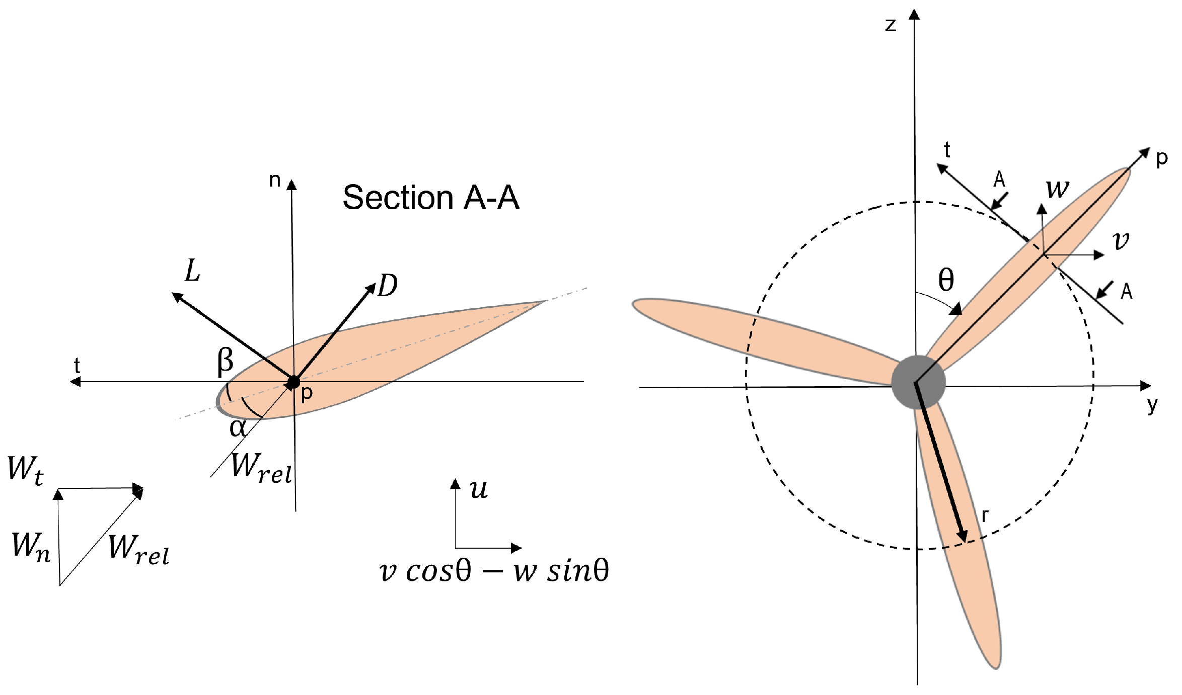
The blade pitch angle is considered constant for all blade sections; moreover, variable values for the local twist angle and the chord along the blade are assumed. More details about the physical model used in the experimentation can be found in [19,20,21].

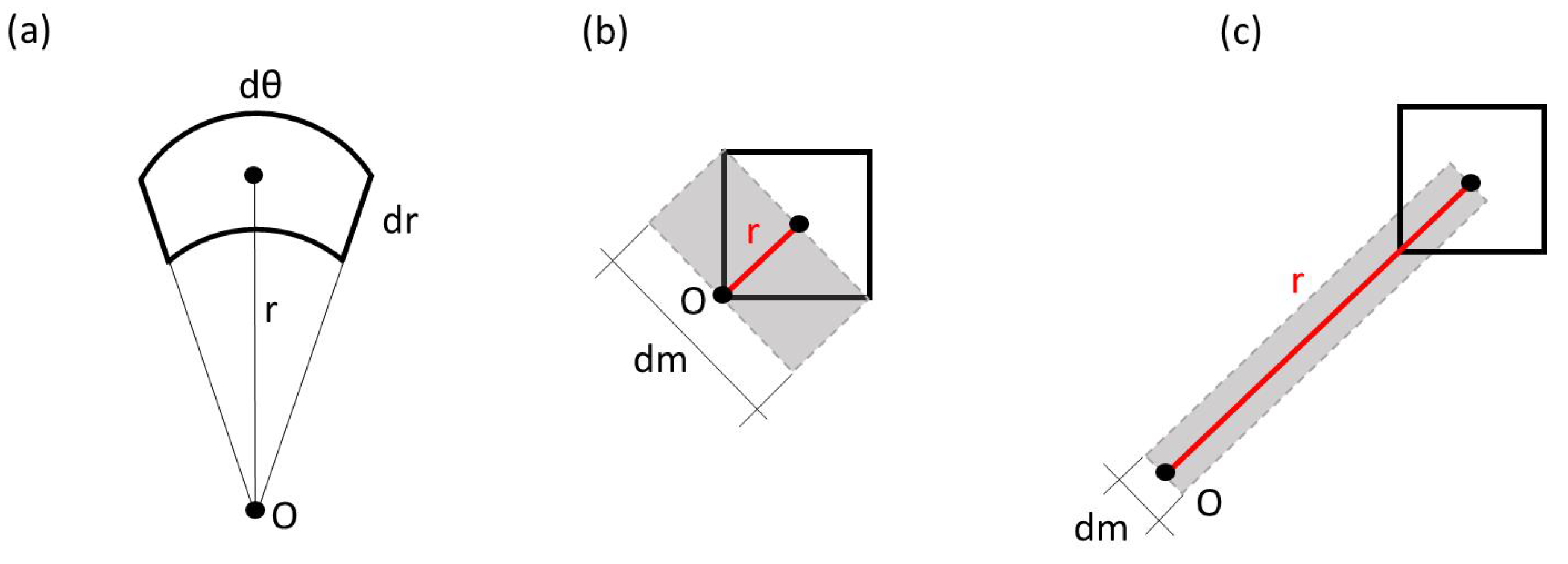
Both grids have variable grid sizes starting from a minimum of 0.05 m in the turbine region to a maximum of 0.5 m.

For the boundary conditions, we impose a constant mass flow rate at the inlet and outlet in order to have the desired undisturbed flow velocity. The top is a free surface, and at the bottom, we consider the free slip condition (i.e., symmetry).

The major difference between the two setups is the hub. Indeed, in SHYFEM, it is not possible to introduce solid bodies along the water column. In the Series 2 campaign, the turbine has a hub diameter equal to one-fifth of the rotor diameter; hence, the rotor effects on the performance and flow field are non-negligible. Thus, in order to account for the hub effect, we reproduced it by locally canceling the speeds. It is a very simplified approach, but it allows the reproduction of the effect of the hub on the surrounding flow field. Hence, we reproduced the presence of the hub by setting all of the velocity components in the three-dimensional space to zero, which should be occupied by the hub. This was the easiest approach that was able to reproduce the hub effect; it does not need a tuning process when changing the case study.

Turbulence Closure

Regarding the turbulence closure, we adopted a slightly different model with respect to the $k-ϵ$ model available in GOTM [22], which is usually used for SHYFEM applications. In this case, we used a one-equation method (for more details about turbulence in marine contexts, please refer to [23]). In such a model, the turbulent kinetic energy (k) is solved using the relative transport equation, while an algebraic relationship is given for the turbulent length scale L. Finally, the eddy viscosity is given as follows:

$${\nu }_t=\frac{C_{\mu }{k}^2}{ϵ}$$

(27)

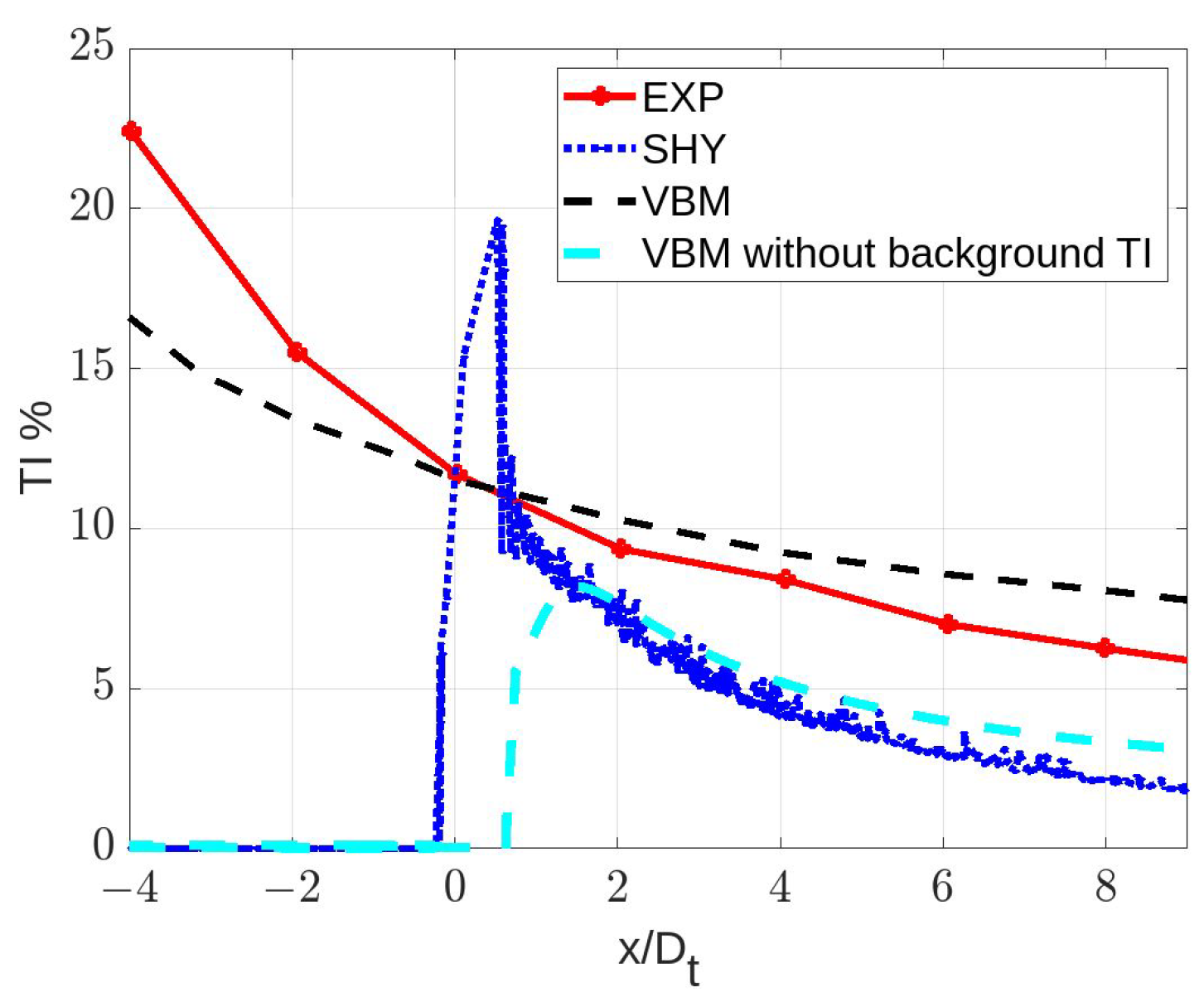
where $C_{\mu }$ is a stability function and $ϵ$ is a function of L. In our case, we adopted the $k-ϵ$ formulation for the k equation, and the ISPRAMIX formulation for L [24]. It is critical to properly model the turbulence, since it strongly affects the wake development, as shown in [21,25].

4. Model Validation

4.1. Performance Validation Series 1

For the SHYFEM turbine validation model, we evaluate the trends of the power coefficient $C_P$ and thrust coefficient $C_T$, defined as follows:

$$C_P=\frac{P}{1/2·\rho ·A_{disc}·U_{\infty }^3}$$

(28)

$$C_T=\frac{T}{1/2·\rho ·A_{disc}·U_{\infty }^2}$$

(29)

where P and T are the power and torque generated, and $A_{disc}$ is the frontal area of the whole turbine. Figure 5a,b show, respectively, the $C_P$ and $C_T$ trends for simulations relative to Series 1 data. The comparison is between the experimental data [19], the SHYFEM model with and without tip losses, and [17] series data, where the same experimental situation is reproduced with VBM in the Ansys Fluent software, with and without tip losses. We can observe good agreement between the SHYFEM model outputs and the other available data. The SHYFEM model is a very accurate BEM-based model, but it is intrinsically simplified due to the hydrostatic assumption. From the turbine perspective, the hydrostatic approach does not allow the introduction of z momentum sources. Indeed, as already anticipated, there is no z-momentum equation. Hence, neglecting a force component, which in a real turbine contributes to the torque and power generation, will inevitably lead to discrepancies in outputs. During the blade revolution, the only position where we do not commit evaluation errors is the vertical position. Indeed, in this position, the z-force component is radial; hence, it does not contribute to torque production. Thus, a trick that we can use to evaluate how turbine behavior appears, in terms of $C_P$ and $C_T$ without the hydrostatic assumption, is to record the local $C_P$ and $C_T$ in the vertical position and then integrate these values over the entire rotor disc area. The results obtained with this procedure are shown in Figure 6a,b.

4.2. Wake Validation Series 2

Regarding the wake validation, we compare results obtained with the Series 2 configuration and set up. In this case, the performance registered with the SHYFEM model (with and without the hub) is in line with the experimental data [21] and VBM Ansys Fluent outputs [17], as shown in Figure 7.

Figure 8 summarizes the wake velocity profiles for three TSR values (2.5, 3.65, and 4.5), and for different diameters ($D_t$) downstream the turbine: 2$D_t$, 3$D_t$, and 4$D_t$. We can see good agreement between the experimental data and the SHYFEM model with the hub for all of the TSRs considered. Indeed, as already anticipated, we cannot neglect the hub effect since its dimension is compared with the rotor diameter. Major differences emerge from 5$D_t$ onward. This is due to the turbulence intensity; indeed, in the experimental campaign, the background turbulence was introduced by means of a grid positioned 8$D_t$ upstream the turbine. The background turbulence intensity in the turbine section amounts to 11.7% (Figure 9). In [17], using the Ansys Fluent software, it was possible to introduce high turbulence in the inlet in order to obtain the desired turbulence intensity in the turbine region, as shown in Figure 9. The dashed black line indicates the turbulence intensity trend for a CFD Ansys Fluent simulation in the absence of the turbine, while the red dotted line indicates the turbulence intensity of the experimental situation without the turbine. Another situation was simulated with Ansys Fluent. All other conditions being equal, we recorded the turbulence intensity obtained without the background turbulence (only due to the turbine’s presence). In this case, the turbulence intensity peak value amounts to about 8%. With the SHYFEM code, it is not possible to introduce external background turbulence, and with the utilized turbulence closure model, we can see a turbulence intensity of about 20% in the turbine region. Analyzing the amount of background turbulence and turbine turbulence, we can reasonably conclude that the SHYFEM model is comparable with the experimental situation in the turbine region. The SHYFEM TM shows a faster drop in turbulence intensity compared to the experiment and Ansys Fluent simulations, resulting in a less-energized wake in SHYFEM from the 5$D_t$ downstream onward.

We return to the hydrostatic assumption as a consequence of the no z-force introduction in the model. The simplification has repercussions in the wake behavior. Indeed, while blades are affected by tangential forces responsible for torque generation, the flow is affected by an equal and contrary force. Hence, the wake flow should start rotating in the opposite direction with respect to the turbine rotational verse. In the SHYFEM TM, it does not happen. We can see that the wake translates instead of rotating, as shown in Figure 10, where the x velocity component is plotted over planes parallel to the rotor plane and located 1$D_t$, 2$D_t$, 3$D_t$, and 4$D_t$ downstream. The arrow indicates the velocity direction parallel to the plane; hence, it is the vector sum of the y and z components. Notice that the y component is predominant in the wake. This is due to the presence of the y-forces and the lack of z-forces. This issue can only be overcome by renouncing the hydrostatic hypothesis. The effect of the wake translation is visible in Figure 8, where the SHYFEM with the hub velocity profile appears a little bit moved with respect to the experimental data. This effect is more evident further from the turbine.

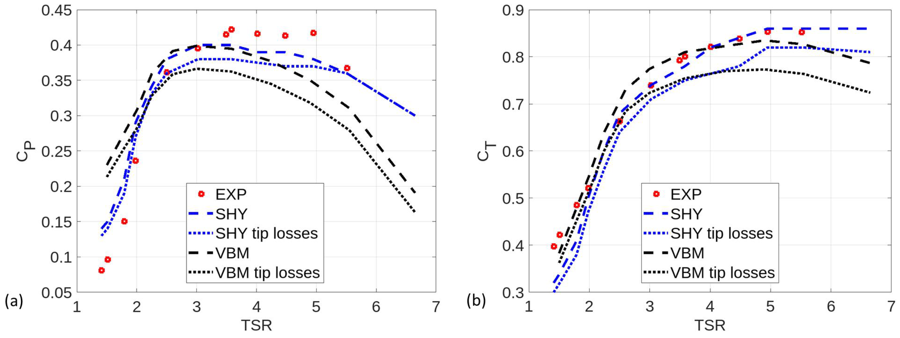
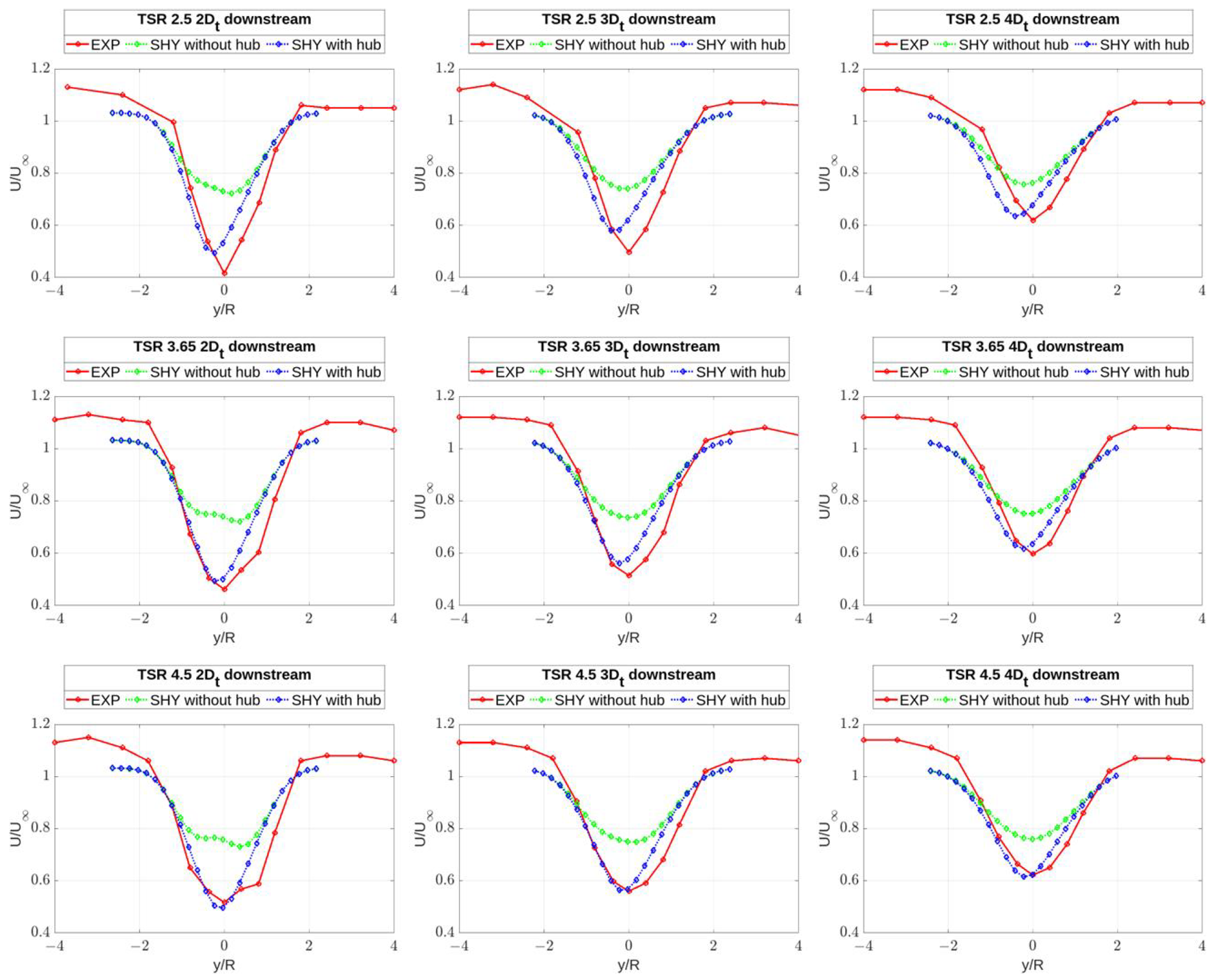
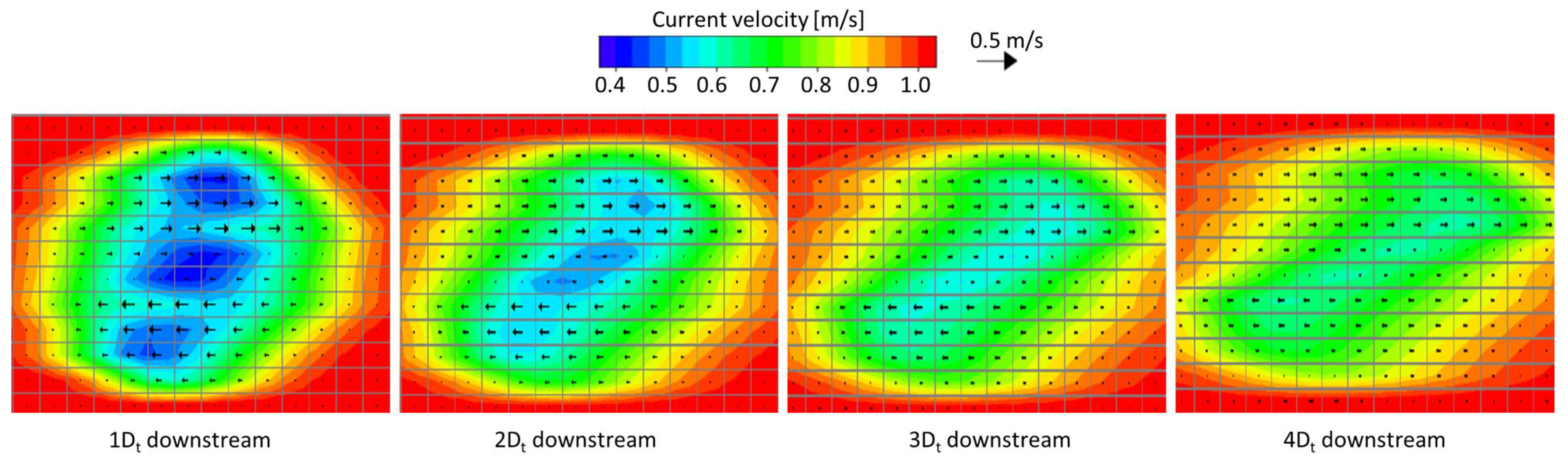
5. Sensitivity Analysis

For the sensitivity analysis, we refer to the Series 2 data, with TSR equal to 3.65. We first compare the results obtained with a fixed horizontal resolution, i.e., 0.05 m in the turbine area, and vary the vertical discretization with several layers of thickness; we analyze three cases: layers of thickness at 0.025, 0.05, and 0.1 m. We observe neglecting variations in the performance parameters (as summarized in

Table 4. Power coefficient with several layer thicknesses and horizontal resolutions.

		Layer			Horizontal
	0.025 m	0.05 m	0.1 m	0.025 m	0.05 m	0.1 m
$C_P$	0.41	0.41	0.42	0.39	0.41	0.40

, where the power coefficient is shown for different layers of thickness). The wake development, shown in Figure 11, is affected little by variations in the layers of thickness in terms of the minimum velocity value in the center of the wake.

Table 5. Percentage difference in the wake centerline velocity with respect to the experimental data. Percentages summarized below are calculated as $(u_{EXP}-u)\ast 100/u_{EXP}$.

		Layer			Horizontal
	0.025 m	0.05 m	0.1 m	0.025 m	0.05 m	0.1 m
$2D_t$	−6.7%	−9.7%	−9.6%	+10.6%	−6.9%	−28.8%
$3D_t$	−10.7%	−10.7%	−9.5%	+6.0%	−8.9%	−24.4%
$4D_t$	−4.0%	4.0%	−1.67%	+10.4%	−3.4%	−15.6%

illustrates the percentage difference in the wake centerline velocity (u) with respect to the experimental data ($u_{EXP}$). No significant variations can be observed by changing the layer thickness. The most relevant difference is that the higher the layer thickness, the more the wake velocity profiles appear translated with respect to experimental data. Indeed, the wake translation is more evident with thicker layers. However, 0.05 m can be assumed as a compromised value between the reliability and computational time saving of the results.

Then, we analyze the sensitivity to the horizontal resolution by varying it in the turbine region. We assume three different resolutions: 0.025, 0.05, and 0.1 m. The vertical discretization is fixed with thickness layers of 0.05 m. The velocity deficit value is strongly affected by the horizontal resolution, as shown in Figure 11 and Table 5; moreover, in this case, a 0.05 m value allows for the best wake reproduction. Table 5 shows that this resolution has the lowest wake velocity percentage difference with respect to the experimental data from 2$D_t$ to 4$D_t$ downstream the turbine. The layer thickness and horizontal resolution have low impacts on the performance output, as shown from the obtained power coefficient summarized in Table 4.

6. Model Application

The TM is now applied to a small farm, made up of ten turbines with realistic sizes. The turbine chosen is geometrically similar to the prototype used in the Series 2 experimentation, but scaled 36 times. Hence, the rotor diameter $D_r$ is 18 m. Firstly, we need to extract the performance curve for the single device. The used domain is 44 $D_r$ long and 12.5 $D_r$ wide. For the depth, we maintained the same blockage of the validation model, i.e., a depth-to-diameter ratio equal to 3.89. The final depth is 72 m and the turbine is located in the middle of the water column. Both horizontal and vertical resolutions are equal to 1 m. The undisturbed flow velocity is set at 1.5 m/s. 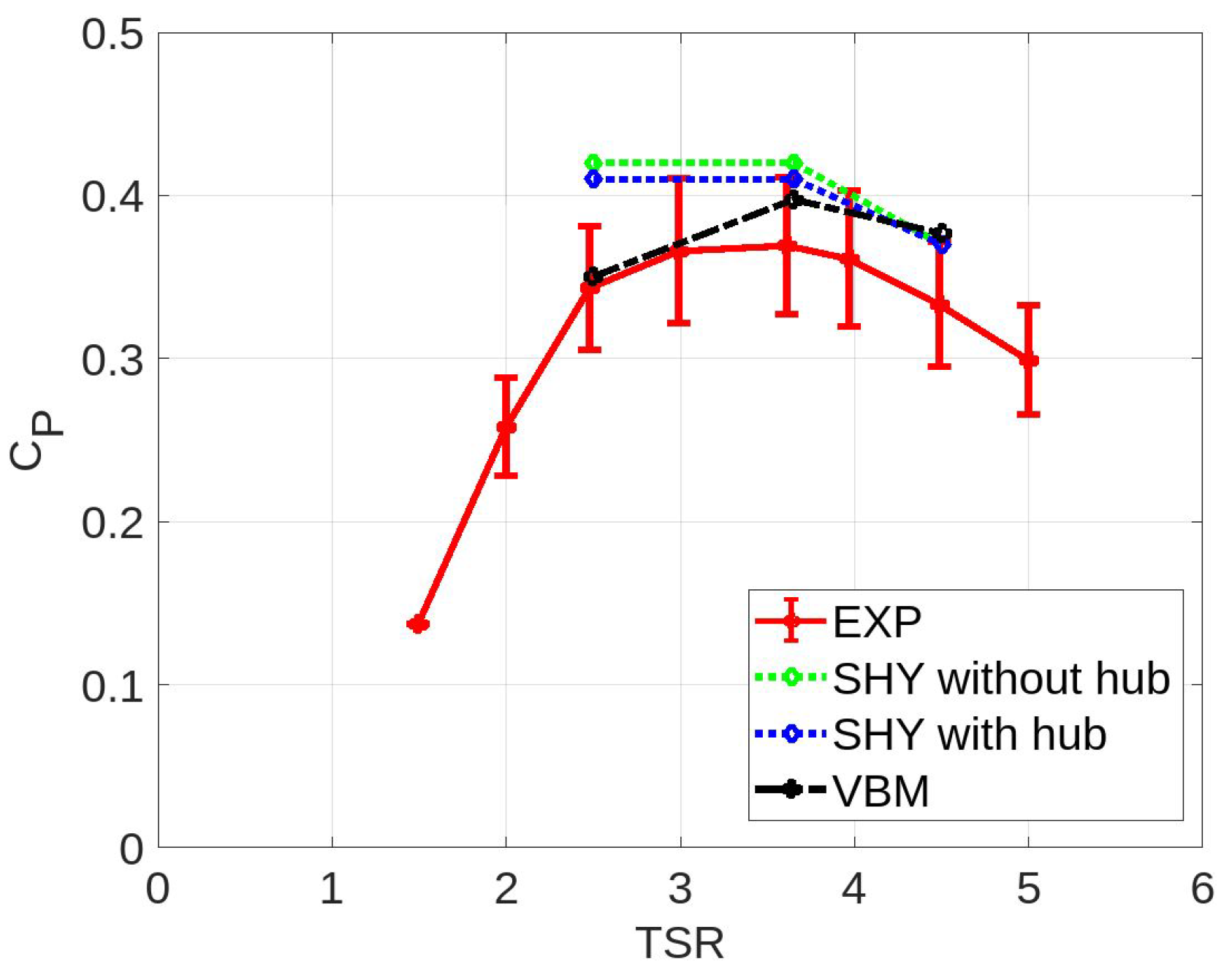The performance curve is shown in Figure 12. Here, we can find the comparison between SHYFEM outputs and results obtained in [26], where CFD simulations were performed at high Reynolds numbers. Indeed, in this work, various situations at high Reynolds numbers were tested and obtained by varying both the rotor diameter and undisturbed flow velocity. Results show that, at high Reynolds numbers, the performance curve collapses into a single curve; see Figure 12. The SHYFEM model performance reaches the same $C_P$ peak value of about 0.39, but the peak is anticipated. Indeed, a TSR of about 3 is reached.

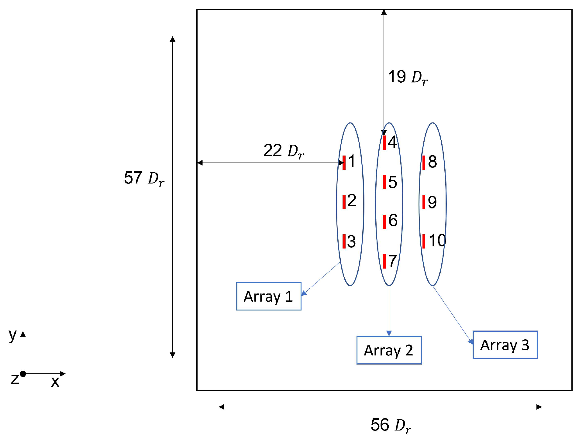
Concerning the farm application, the devices are laterally and longitudinally spaced by six diameters, and are located in a staggered configuration, as shown in Figure 13. According to the literature, the staggered configuration is preferable for higher energy exploitation ([27,28]), so we opted for this layout, as it prevents the wake of an array from impacting the immediately following array. Moreover, this layout allows the following array to benefit from the accelerated flow due to the mutual blockages of adjacent turbines. The domain in this case is 56 $D_r$ long and 57 $D_r$ wide; all other parameters are equal to those used for the single-device test.

The aim of this application is to show the potentiality of our model. For this purpose, we evaluate five different situations:

• BASE: the BASE configuration is exactly the same as the one shown in Figure 13, with th turbine laterally and longitudinally spaced at 6$D_r$.
• 3$D_r$: this is a variation of the BASE, where Array 2 is spaced 3$D_r$ from Array 1; the lateral space between the devices is still 6$D_r$.
• 9$D_r$ A: this is a variation of the BASE, where Array 2 is spaced 9$D_r$ from Array 1; the lateral space between devices is still 6$D_r$.
• 9$D_r$ B: this is the same spatial layout as case 9$D_r$ A, with further rotational speed adaptation for Array 3.
• 9$D_r$ C: this is the same spatial layout as case 9$D_r$ A, with depth variation for Array 3.

All of these configurations globally occupy the same horizontal marine area. For the test BASE, 3$D_r$, 9$D_r$ A, and 9$D_r$ C, all of the devices are operated with optimal TSRs, i.e., 3. The rotational speed is obtained via the TSR definition (Equation (26)), using an undisturbed flow velocity of 1.5 m/s. Performances are summarized in

Table 6. Performance of each turbine inside the farm in the five different configurations. $\Delta P_{tot}$ is calculated as ($P_{tot}$−$P_{BASE}$)·100/$P_{BASE}$.

Turbine	1	2	3	4	5	6	7	8	9	10
	${\mathbf{C}}_{\mathbf{P}}$	${\mathbf{C}}_{\mathbf{P}}$	${\mathbf{C}}_{\mathbf{P}}$	${\mathbf{C}}_{\mathbf{P}}$	${\mathbf{C}}_{\mathbf{P}}$	${\mathbf{C}}_{\mathbf{P}}$	${\mathbf{C}}_{\mathbf{P}}$	${\mathbf{C}}_{\mathbf{P}}$	${\mathbf{C}}_{\mathbf{P}}$	${\mathbf{C}}_{\mathbf{P}}$	$\Delta {\mathbf{P}}_{\mathbf{tot}}$
BASE	0.38	0.38	0.39	0.39	0.40	0.40	0.38	0.25	0.24	0.25	/
3$D_r$	0.38	0.38	0.39	0.39	0.40	0.40	0.38	0.26	0.25	0.26	+1%
9$D_r$ A	0.39	0.38	0.39	0.39	0.40	0.40	0.39	0.26	0.25	0.26	+1%
9$D_r$ B	0.39	0.38	0.39	0.39	0.40	0.40	0.39	0.27	0.26	0.27	+2%
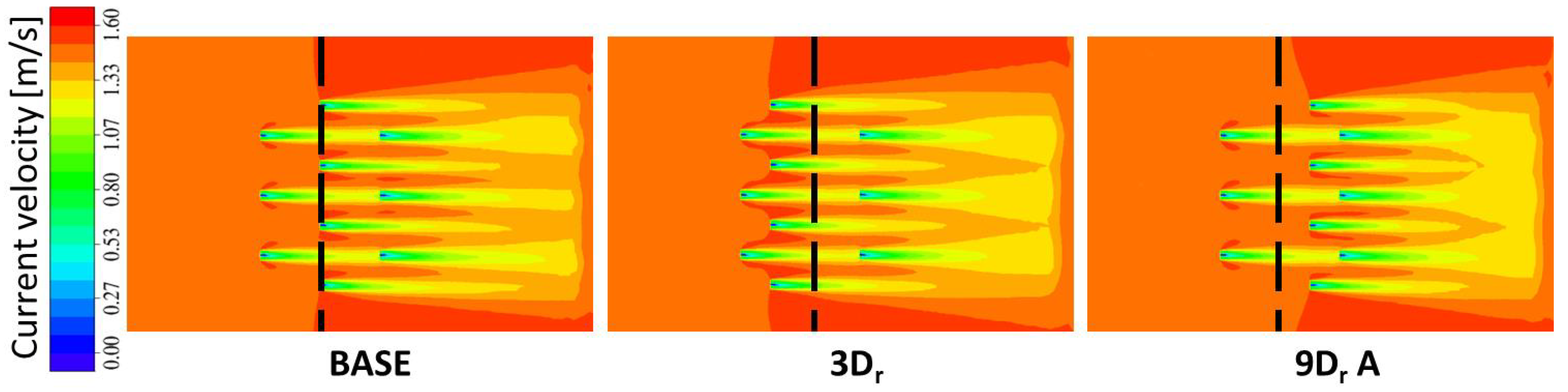
9$D_r$ C	0.39	0.38	0.39	0.39	0.40	0.40	0.39	0.29	0.29	0.30	+5%

. We can see that, for all studied configurations, turbines 5 and 6 benefit from the flow deviation due to the presence of Array 1 turbines. Indeed, they are more beneficially influenced by acceleration corridors (Figure 14). The latter arises between adjacent turbines due to the blockage effect offered by each device to the incoming flow. The flow senses the turbine as an obstacle and, hence, tends to deviate in the radial direction with respect to the turbine axis.

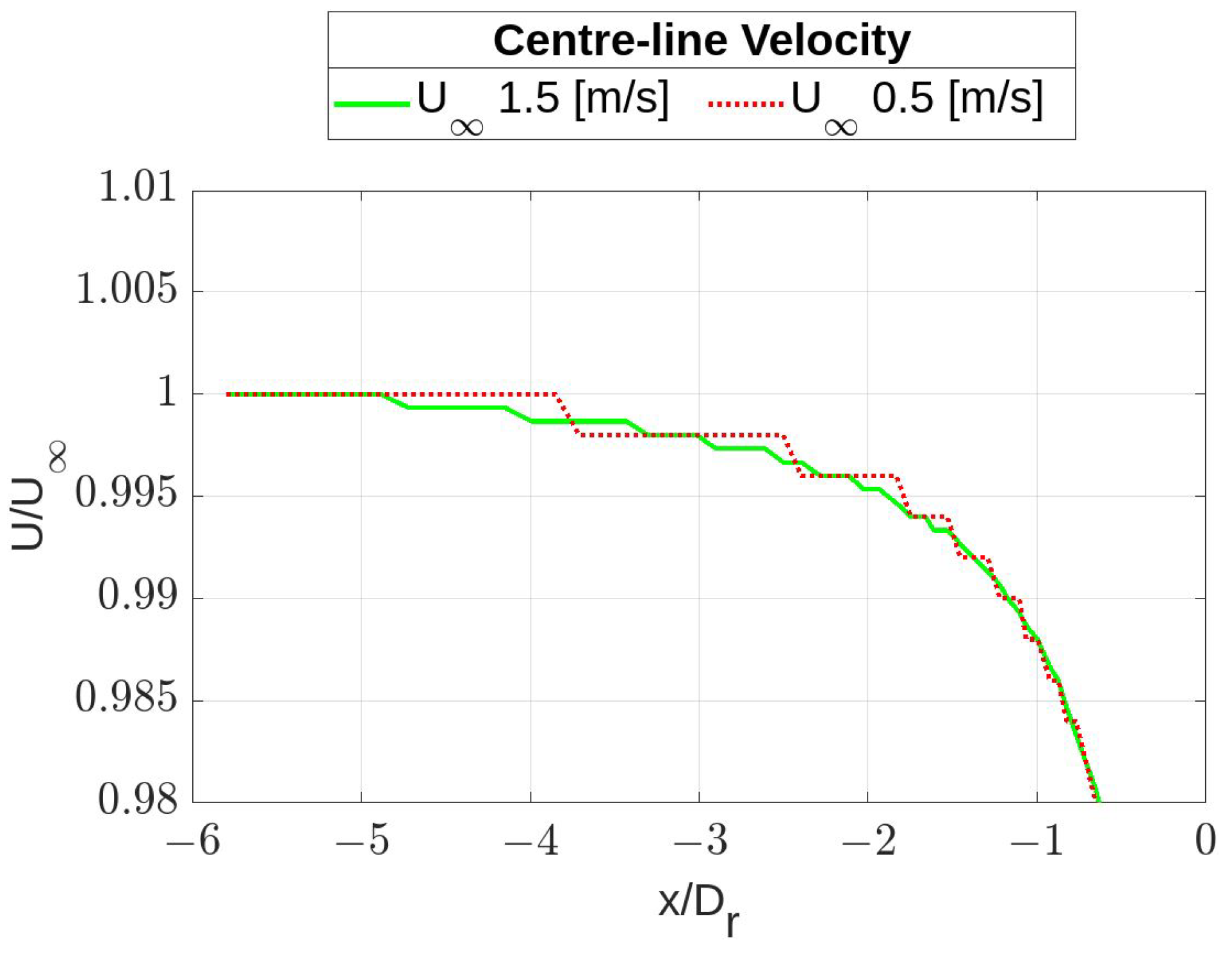
In 9$D_r$ B, we evaluate changes in the operational conditions of the farm by independently adapting the rotational speed of every single device. Since arrays located downstream are reached by lower flow velocities, it is important to adapt the rotational speed via optimal TSR using a proper reference velocity. Array 1 is reached by the undisturbed flow velocity but the others are reached by different velocities. Using a unique $\Omega$ value for all devices is similar to imposing on those located downstream, working at a higher TSR. It is necessary to establish where to measure the reference velocity. To this end, we evaluated the flow velocity upstream by simulating the single device at the optimal TSR and in two flow conditions: with flow velocities of 1.5 and 0.5 m/s. The former is the undisturbed flow velocity chosen for the farm application; the latter is a potential cut in the velocity; furthermore, it is the result of the wake velocity ($U_{wake}$) evaluation following the actuator disc theory, calculated in the idealized case of the axial induction factor a, equal to 1/3. Hence, the wake velocity, which would reach the downstream arrays, is 0.5 m/s, following Equation (30).

$$U_{wake}=(1-a)U_{\infty }$$

(30)

Figure 15 shows the centerline velocity profile, with dimensionless velocities plotted. For both undisturbed velocities, we can consider the distance of 5$D_r$ from the turbine center as the upstream distance to measure the reference velocity. Indeed, in both flow velocity conditions, this distance is close enough to the turbine to detect the effective incoming flow velocity, but not so close as to be affected by the axial induction factor of the turbine itself.

From 9$D_r$ A, we evaluate the 5$D_r$ upstream velocity for turbines 8, 9, and 10, and use them to adapt the rotational speed at the optimal TSR. The new rotational speed is 0.4 rad/s for the three devices, instead of 0.5 rad/s. This adaptation leads to an increase in the power production of 5% with respect to the BASE case. The $\Omega$ adaptation was done only for Array 3, because it is the only one reached by a disturbed flow velocity. Indeed, for Array 2, the 5$D_r$ upstream velocity is equal to 1.5 m/s. The power increment is slight since the performance curve near the peak value is quite flat; hence, no dramatic drop in power production occurs if we deviate a little from the optimal TSR value. However, this procedure gives the strategy on how to best perform on a farm by adapting to the working conditions of each device.

A further analysis concerns the depth of the turbines. So far, we have analyzed a 10-turbine cluster, where all the devices were located at the same depth. Case 9D C shows an application where Array 3 is located half a radius higher than the other two; moreover, in this case, we act only on Array 3, since it is “one more” negatively affected by the presence of the others. We can see an improvement in performance for Array 3, and an overall increment in the power production of +5% with respect to the BASE case as shown in Table 6, where $\Delta P_{tot}$ indicates the difference in the farm’s total power production of each configuration ($P_{tot}$) compared to the BASE case, normalized with the BASE case power ($P_{BASE}$). These results are in line with the literature [29]. The latter case highlights the 3D character of the SHYFEM TM, while the BEM approach allows evaluating mutual influence between devices.

From Table 6, one can see that some devices work with performances higher than the maximum value of 0.39 reached by the single device (Figure 12). This phenomenon can be explained by the mutual influence of the devices on each other, in particular with the acceleration corridors that arise between turbines.

7. Conclusions

In this work, we developed a 3D horizontal axis turbine model within the SHYFEM open-source marine code. The model is a BEM-based one and was validated for performance prediction and wake development against experimental data found in [19,21], respectively. The model is equipped with a tip loss sub-model in order to reproduce the 3D phenomenon. Despite the extreme simplicity of the implemented model, and the assumptions made, it allows the reproduction of the behavior of the turbine with satisfactory accuracy. The model’s simplification can be summarized as follows: approximated rotor disc area, due to the finite element grid generation; the impossibility of inserting a solid hub is replaced by imposing zero-axial velocity in the hub location; the hydrostatic approximation, which implies neglecting the z-source terms of the turbine.

The model was applied to a small cluster of 10 turbines, with realistic sizes. For the case study, the performance comparison against CFD data [26] showed that the model had a good response with varied parameters, particularly by evaluating a high Reynolds number. From the small farm application, we saw the potentiality of the model in the performance evaluation in terms of changes in the horizontal layout, changes in the vertical layout, and changes in the operational parameters for each device; in particular, we evaluated the influence of $\Omega$ in a sort of maximum power tracking strategy. The TM allows reproducing high Reynolds number situations with limited computational time costs. We spent about 10 h to simulate the cluster with a domain large enough to be considered unlimited. At the same time, the BEM character of the TM allows for capturing mutual influences between the devices (for instance, acceleration corridors), and changes in operational or geometrical parameters, giving highly accurate responses. In this sense, the SHYFEM model attempts to cover the knowledge gap in the available data, reproducing (with a sufficient degree of accuracy) high Reynolds number situations, evaluating realistically sized devices, reproducing realistic flow conditions, and simulating elevated numbers of devices, such as those on a farm (we chose 10 turbines for this application, but the TM allows reproducing the desired number of devices). Therefore, we will be able to test situations that would be prohibited for both CFD simulations and experimental in situ campaign, with a sufficient degree of accuracy, and considering realistic in situ conditions (i.e., flow velocity, tide, wave, wind, bathymetry, coast morphology, salinity, temperature, and so on). The TM could be a useful tool for hydrokinetic turbine farm studies, both from a power production optimization point of view and from an environmental impact point of view, in terms of sediment transport, for instance.

References

1. Magagna, D. Ocean Energy Technology Development Report 2018, EUR 29907 EN; JRC118296; European Commission: Luxembourg, 2019; ISBN 978-92-76-12428-3. [CrossRef]
2. McNaughton, J.; Cao, B.; Ettema, S.; Zilic de Arcos, F.; Vogel, C.R.; Willden, R.H.J. Experimental testing of the performance and interference effects of a cross-stream array of tidal turbines. In Developments in Renewable Energies Offshore; CRC Press: London, UK, 2020; pp. 1–8. [Google Scholar]
3. Noble, D.R.; Draycott, S.; Nambiar, A.; Sellar, B.G.; Steynor, J.; Kiprakis, A. Experimental Assessment of Flow, Performance, and Loads for Tidal Turbines in a Closely-Spaced Array. Energies 2020, 13, 1977. [Google Scholar] [CrossRef]
4. Nuernberg, M.; Tao, L. Experimental study of wake characteristics in tidal turbine arrays. Renew. Energy 2018, 127, 168–181. [Google Scholar] [CrossRef] [Green Version]
5. Zhang, C.; Kramer, S.C.; Angeloudis, A.; Zhang, J.; Lin, X.; Piggott, M.D. Improving tidal turbine array performance through the optimisation of layout and yaw angles. In Proceedings of the 14th European Wave and Tidal Energy Conference, Plymouth, UK, 5–9 September 2021. [Google Scholar]
6. Plew, D.R.; Stevens, C.L. Numerical modelling of the effect of turbines on currents in a tidal channel—Tory Channel, New Zealand. Renew. Energy 2013, 57, 269–282. [Google Scholar] [CrossRef]
7. Kramer, S.C.; Piggott, M.D. A correction to the enhanced bottom drag parameterisation of tidal turbines. Renew. Energy 2016, 92, 385–396. [Google Scholar] [CrossRef] [Green Version]
8. Piano, M.; Robins, P.E.; Davies, A.G.; Neill, S.P. The Influence of Intra-Array Wake Dynamics on Depth-Averaged Kinetic Tidal Turbine Energy Extraction Simulations. Energies 2018, 11, 2852. [Google Scholar] [CrossRef] [Green Version]
9. Marsh, P.; Penesis, I.; Nader, J.R.; Couzi, C.; Cossu, R. Assessment of tidal current resources in Clarence Strait, Australia including turbine extraction effects. Renew. Energy 2021, 179, 150–162. [Google Scholar] [CrossRef]
10. Ramos, V.; Carballo, R.; Ringwood, J.V. Application of the actuator disc theory of Delft3D-FLOW to model far-field hydrodynamic impacts of tidal turbines. Renew. Energy 2019, 139, 1320–1335. [Google Scholar] [CrossRef]
11. Djama Dirieh, N.; Thiébot, J.; Guillou, S.; Guillou, N. Blockage Corrections for Tidal Turbines—Application to an Array of Turbines in the Alderney Race. Energies 2022, 15, 3475. [Google Scholar] [CrossRef]
12. Soto-Rivas, K.; Richter, D.; Escauriaza, C. Flow effects of finite-sized tidal turbine arrays in the Chacao Channel, Southern Chile. Renew. Energy 2022, 195, 637–647. [Google Scholar] [CrossRef]
13. SHYFEM Model-GitHub. Available online: Https://github.com/SHYFEM-model (accessed on 13 July 2022).
14. Zori, L.; Rajagopalan, G.R. Navier-Stokes Calculation of Rotor-Airframe Interaction in Forward Flight. J. Am. Helicopter Soc. 1995, 40, 57–67. [Google Scholar] [CrossRef]
15. Kundu, P.K.; Cohen, I.M. Geophysical Fluid Dynamics. In Fluid Mechanics, 2nd ed.; Elsevier Science (USA); Academic Press: San Diego, CA, USA, 2002; pp. 555–627. [Google Scholar]
16. Shen, W.Z.; Zhu, W.J.; Sørensen, J.N. Study of tip loss corrections using CFD rotor computations. J. Phys. Conf. Ser. 2014, 555, 012094. [Google Scholar] [CrossRef]
17. Lombardi, N.; Ordonez-Sanchez, S.; Zanforlin, S.; Johnstone, C. A Hybrid BEM-CFD Virtual Blade Model to Predict Interactions between Tidal Stream Turbines under Wave Conditions. J. Mar. Sci. Eng. 2020, 8, 969. [Google Scholar] [CrossRef]
18. Lombardi, N. Hybrid BEM-CFD Virtual Blade Model to Investigate the Interaction between Two Marine Turbines under Tidal Current and Wave Conditions. Master’s Thesis, University of Pisa, Pisa, Italy, 2020. [Google Scholar]
19. Ordonez-Sanchez, S.; Allmark, M.; Porter, K.; Ellis, R.; Lloyd, C.; Santic, I.; O’Doherty, T.; Johnstone, C. Analysis of a Horizontal-Axis Tidal Turbine Performance in the Presence of Regular and Irregular Waves Using Two Control Strategies. Energies 2019, 12, 367. [Google Scholar] [CrossRef] [Green Version]
20. Allmark, M.; Ellis, R.; Lloyd, C.; Ordonez-Sanchez, S.; Johannesen, K.; Byrne, C.; Johnstone, C.; O’Doherty, T.; Mason-Jones, A. The development, design and characterisation of a scale model Horizontal Axis Tidal Turbine for dynamic load quantification. Renew. Energy 2020, 156, 913–930. [Google Scholar] [CrossRef]
21. Ebdon, T.; Allmark, M.J.; O’Doherty, D.M.; Mason-Jones, A.; O’Doherty, T.; Gregory, G.; Gaurier, B. The impact of turbulence and turbine operating condition on the wakes of tidal turbines. Renew. Energy 2021, 165, 96–116. [Google Scholar] [CrossRef]
22. GOTM. Available online: Https://gotm.net/ (accessed on 15 August 2018).
23. Burchard, H. Applied Turbulence Modelling in Marine Waters. In Lecture Notes in Earth Sciences; Bhattacharji, S., Friedman, G.M., Neugebauer, H.J., Seilacher, A., Eds.; Springer: Berlin/Heidelberg, Germany, 2002. [Google Scholar]
24. Eifler, W.; Schrimpf, W. ISPRAMIX, a Hydrodynamic Programme for Computing Regional Sea Circulation Patterns and Transfer Processes: Description of the Model Equations and of the Solution Procedure; CEC Report EUR 14856 EN; 1992. [Google Scholar]
25. Gaurier, B.; Carlier, C.; Germain, G.; Pinon, G.; Rivoalen, E. Three tidal turbines in interaction: An experimental study of turbulence intensity effects on wakes and turbine performance. Renew. Energy 2020, 148, 1150–1164. [Google Scholar] [CrossRef]
26. Mason-Jones, A.; O’Doherty, D.M.; Morris, C.E.; O’Doherty, T.; Byrne, C.B.; Prickett, P.W.; Grosvenor, R.I.; Owen, I.; Tedds, S.; Poole, R.J. Non-dimensional scaling of tidal stream turbines. Energy 2012, 44, 820–829. [Google Scholar] [CrossRef]
27. Draper, S.; Nishino, T. Centred and staggered arrangements of tidal turbines. J. Fliud Mech. 2014, 739, 72–93. [Google Scholar] [CrossRef]
28. Nguyen, V.T.; Santa Cruz, A.; Guillou, S.S.; Shiekh Elsouk, M.N.; Thiébot, J. Effects of the Current Direction on the Energy Production of a Tidal Farm: The Case of Raz Blanchard (France). Energies 2019, 12, 2478. [Google Scholar] [CrossRef]
29. Vasel-Be-Hagh, A.; Archer, C.L. Wind farm hub height optimization. Appl. Energy 2017, 195, 905–921. [Google Scholar] [CrossRef]
Figure 1. Qualitative representation of the forces acting on a blade element, located at a generic radius r, and shown from section A-A.
Jmse 10 01864 g001
Figure 2. (a) SHYFEM grid details; the yellow rectangle delimits the turbine’s top view, (b) qualitative representation of the turbine’s frontal area in the SHYFEM z-layer discretization, and (c) details of a typical ANSYS Fluent grid used with VBM.
Jmse 10 01864 g002
Figure 3. (a) Regular grid element of the turbine (typical of VBM applications), (b) qualitative representation of a turbine element located near the center O for an irregular grid, and (c) qualitative representation of a turbine element located far from the center O for an irregular grid.
Jmse 10 01864 g003
Figure 4. Qualitative representation of the free surface displacement across the turbine. H is the water column undisturbed depth; the free surface displacement is emphasized for explanatory purposes.
Jmse 10 01864 g004
Figure 5. (a) C P T S R and (b) C T T S R curves; comparison between experimental data (red squares), Ansys Fluent VBM model without tip losses (dashed black line), with tip losses (dotted black line), the SHYFEM model without tip losses (dashed blue line), and with tip losses (dotted blue line).
Jmse 10 01864 g005
Figure 6. (a) C P T S R and (b) C T T S R curves; comparison between the SHYFEM TM (dashed blue line) and the integration of vertical values over the entire rotor disc area (pink dot).
Jmse 10 01864 g006
Figure 7. C P T S R curve; comparison between experimental data, VBM Ansys Fluent model, and SHYFEM TM with and without the hub.
Jmse 10 01864 g007
Figure 8. Wake velocity profiles for different downstream TSRs at 2 D t , 3 D t , and 4 D t . Comparison between experimental data (red line) and the SHYFEM model with (green line) and without (blue line) the hub.
Jmse 10 01864 g008
Figure 9. Turbulence intensity percentage in the experimental situation and CFD ANSYS Fluent (only the background turbulence—red and black dashed lines, respectively), a VBM Ansys Fluent simulation, and a SHYFEM simulation (turbine-only turbulence—light blue dashed and blue dotted lines, respectively).
Jmse 10 01864 g009
Figure 10. The x velocity field on planes parallel to the rotor disc plane, several diameters downstream. The arrows indicate the velocity direction of the plane, i.e., the vector sum of y and z components.
Jmse 10 01864 g010
Figure 11. Wake velocity profile at TSR 3.65 2 D t , 3 D t , and 4 D t downstream of the turbine for different spatial discretizations; various layer thicknesses (top) and various horizontal resolutions (bottom).
Jmse 10 01864 g011
Figure 12. C P T S R curve for the single device.
Jmse 10 01864 g012
Figure 13. Qualitative representation for the ten-turbine farm, with staggered configuration.
Jmse 10 01864 g013
Figure 14. Flow field in the mid-plane of turbines for the case BASE, 3 D r , and 9 D r A.
Jmse 10 01864 g014
Figure 15. Dimensionless velocity along the centerline approaching the turbine considering two different flow undisturbed velocities: 1.5 and 0.5 m/s. The x axis represents the dimensionless x coordinate, and the turbine is located in x / D r , equal to zero.
Jmse 10 01864 g015