Abstract
Taiwan is surrounded by sea; therefore, coastal hazards might become severe due to climate change. The analysis of wave climate characteristics at different time scales (long-term historical period, seasonal prediction, and future prediction) can be used as a reference for the impact of climate change on coastal environments. This model associates the significant wave height with the atmospheric predictor defined by the sea level pressure (SLP) field. We applied SLP based on the outputs of a global climate model (GCM) under two possible future scenarios (RCP4.5 and RCP8.5) in the Fifth Assessment Report, AR5 (IPCC, 2014), then used the historical data of the predictor (sea level pressure) and predictand (sea-state parameters) from reanalysis databases to calibrate the model. The recent historical atmospheric conditions responsible for the swell wave component at the target site are included in the predictor definition. The 18 days sea level pressure fields are used as a predictor by utilizing the evaluation of source and travel-time of wave energy reaching a local area (ESTELA) method. The verification proves the model’s skill to reproduce the seasonal and interannual variability of monthly sea state parameters and can be used to further evaluate the wave climate change around Taiwan under different climate change scenarios. The prediction of wave climate on weather types provides a physical explanation for the relationship between the multivariate wave climate characterization and atmospheric forces. Through the analysis of the similarity and consistency between GCM data and reanalysis data, we can evaluate the suitability of GCM for wave climates in the Taiwan sea area. It shows how the weather type statistical method can be used to quantify the wave climate prediction results of each GCMs and to evaluate their differences and uncertainties, which will improve the estimation of the impact of wave climate change on Taiwan’s coast.
1. Introduction
Climate change across the globe has a substantial impact on the oceans by bringing variations in sea levels, waves, and weather conditions. The coastal areas have become vulnerable due to the elevated strength of ocean waves and the frequent occurrence of giant waves. The statistical downscaling framework proposed by Camus et al. [1]. is adopted to gain wave data with a higher resolution. For instance, larger waves can cause severe erosion and inundation of the coastlines exposed due to climate change [2,3]. In recent years, researchers have reported a consistent increase in wave height in the North Pacific oceans [4]. Taiwan, a sub-tropical island located at the western boundary of the North-Pacific, is also experiencing wave climate variability [4]. In particular, seasonal wave climate changes directly affect the topographic changes in coastal areas and cause erosion disasters. The wave conditions in the oceans are related to regional weather systems and, thus, directly impact the wave climate. Therefore, for coastal hazard mitigation pertaining to climate change to provide insights for policymaking, making it is crucial to project wave conditions and understand the future variations in the sea around Taiwan.
Currently, analysis of wave climate variability as a result of climate change and the projection of future scenarios includes the simulation results of global climate models (GCMs) provided by the Intergovernmental Panel on Climate Change (IPCC). The major limitation of the simulations is insufficient spatial resolution, resulting in a lack of detailed local climate information. In turn, this causes difficulty in obtaining reliable future projections at a regional scale. Hence, the ideal possible approach to overcome the issue can be downscaling. The future wave climate projection can adopt either dynamic (DD) or statistical downscaling (SD) simulations. DD has been applied by Mori, Yasuda [5], Hemer, Fan [6], Semedo, Weisse [7], and Laugel, Menendez [8] to the global climate. DD is useful in generating finer and more reliable climate information by incorporating more complex topography to better reproduce the physical response to the large-scale atmospheric information from GCM results [9]. However, the trade-off is a long simulation time and involves expensive computational resources [1,9].
Unlike DD, the significantly lower computational time of SD provides the advantage of projecting many GCMs, providing simulation results and uncertainty assessments for various scenarios [9]. Hence, SD is considered a more robust method for reproducing seasonal means and extremes [8]. SD also overcomes the other limitation of DD, which is diminishing the model bias by the standardization of the predictor [8,9]. SD has been applied at both global and regional levels to projections of sea wave heights, sea level pressure fields, and sea surface winds. However, the extreme values projected using regression models are often limited to significant wave heights. As a result, Camus, Menendez [1] proposed a framework for the weather type of statistical downscaling, extending the analysis to more variables. SD defines a linear [10] or nonlinear relationship between the atmospheric variables and wave parameters. In those works, the predictor for the daily total bulk wave parameters at a particular location was defined by daily regional sea level pressure (SLP) fields averaged over an optimal number of days. In addition, Perez, Mendez [11] utilized ESTELA to identify the spatial range of the predictor that covered the primary areas of wave generation for the location. This method has been applied extensively with success in smaller ocean basins, such as the North Atlantic and Mediterranean Oceans [8,12,13,14]. Hegermiller, Antolinez [15] pointed out that the characteristic propagation time of wave energy to the target area must be considered when using ESTELA to establish a predictor in a large ocean basin such as the Pacific Ocean. This method requires low-resolution atmospheric data and high-resolution wave data and setting up a statistical model with long-term data. From the statistical relation between atmospheric and wave data, detailed spatial information can be obtained directly, whose resolution depends on the statistical model’s wave data.
The present study aims to apply the weather type-downscaling model for the coastal waters around Taiwan to shed light on the impact of climate change on future wave climates and changes in significant wave height. Considering the monsoon climate of Taiwan, the analysis is carried out in a specific location in the southwest of Taiwan and conducted for different seasons. This location is one of the coasts with the fastest topographic changes in Taiwan at present, and there is an observation site, “THL2B”, that can provide measured wave data for analysis and verification. The atmospheric reanalysis data provided by the National Center for Environmental Prediction (NCEP) and the National Center for Atmospheric Research (NCAR), along with the wave reanalysis data (ERA5) provided by the European Centre for Medium-Range Weather Forecasts (ECMWF), are used to create a statistical model aiming to simulate various scenarios using multiple GCMs.
2. Statistical Downscaling Method
The SD method evaluates local waves (predictand) at high resolution from low-resolution atmospheric (predictor) conditions based on a statistical relation. In this study, the weather type SD proposed by Camus, Menendez [1] is used to establish the relationship between the predictand and predictor in the statistical model. The main framework is summarized in Figure 1. The detailed steps are:
- The collection of historical reanalysis data, comprising atmospheric data and wave data.
- Using and evaluating the source and travel time of the wave energy reaching a local area (ESTELA) method proposed by Perez, Mendez [11]. Defining the spatial domain in the model and the predictor on a daily scale.
- Clustering the atmospheric conditions into several weather types using the k-means algorithm in the reference period.
- The association of weather types with the local wave data is based on their statistical relationship, which does not change over time.
- The validation or projection from reanalysis or measured data and GCMS data, respectively, obtaining the wave distribution in a unit of time (e.g., monthly, annual) from sea states and the occurrence probability, which is the only variable for each weather type.
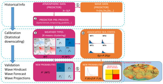
Figure 1.
Framework of the statistical downscaling approach.
To avoid observations with missing data, reanalysis data (ERA5) from numerical simulations are used. The correlation between the reanalysis data and the measured data is as high as 0.92 (Figure 2), so this data is considered to be quasi-real data.
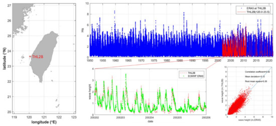
Figure 2.
The location of THL2B site and correlation between the reanalysis data and the measured data.
In the model, atmospheric data is defined as the sea level pressure, and wave data is defined as the significant wave height. The spatial domain of the predictor is specified using the ESTELA method [11], which finds the area of a swell generation that reaches a particular location based on an evaluation of energy and travel time. Additionally, atmospheric conditions should include the propagation processes of waves so that the predictor is averaged from the previous days and defined on the daily scale according to the travel time of ESTELA. The weather type is then determined by clustering. The clustering technique is based on two methods. First, a principal component analysis (PCA) is used to concentrate the variables and reduce data dimensionality [16]. PCA defines a new space from the original data using eigenvalues and eigenvectors whose components are orthogonally related. The covariance of the elements is zero, and thus, each variable is independent in the new space. Then, the new space predictor is clustered using the k-means algorithm and grouped into several clusters. Each cluster is formed by the similarity minimized Euclidean distance of data and is represented by a centroid defined as the mean in each group [17]. The sea state is then associated at the location of interest with the corresponding weather type, establishing the empirical relationship between the atmospheric conditions and wave climate and allowing a non-linear relationship. The empirical relationship is established for a reference period and presented in the probability distribution of the variable in Figure 1 (e.g., significant wave height () in this study). The distribution of can be evaluated for the whole reference period as follows:
where is the probability of the corresponding weather type (). The occurrence probability of is calculated from a number of daily predictors in the cluster of , so that , where M is the number of weather types. For validation or projection, the atmospheric conditions are affected by the weather type because the time period is outside the reference period. The new occurrence probability is obtained from the weather types by clustering. The new distribution of can be estimated as:
Finally, to ascertain the applicability of the statistical downscaling model, the model is validated for the monthly mean of based on the distribution associated with each and the occurrence probability for a given period.
3. Model Settings and Validation
3.1. Predictor
In this study, the predictors for the ocean waves were sea level pressure (SLP) and the squared SLP gradient (SLPG) [18]. SLP and SLPG are used to find the propagation processes of swells generated far away and establish a relationship between atmospheric conditions and the waves [12]. The NCEP provides reanalysis data spanning from 1948 to the present. The data consist of six hourly fields whose spatial resolution is a 2.5° by 2.5° long.-lat. global grid. As in Hegermiller, Antolinez [15], we build up the predictor from the SLP and SLPG by accounting for the isochrones (the characteristic travel time of the wave energy to the target area, the gray and black lines in Figure 3 and Figure 4),
where is the spatial domain, is time, is the domain between the daily isochrones and , and is the number of days for the longest wave propagation time from generation until arrival at the target location (18 days in this work). We emphasize that with this approach, we keep track of the geostrophic wind conditions that generate waves affecting the target location.
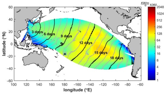
Figure 3.
Mean effective energy flux obtained using ESTELA method from 1980 to 2004 in the east of Taiwan.
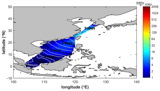
Figure 4.
Mean effective energy flux obtained using ESTELA method from 1980 to 2004 in the west of Taiwan.
3.2. Predictand
The statistical model requires the local wave climate parameter to be the predictand. The significant wave height data obtained from the latest reanalysis production ERA5 of ECMWF are used. The ERA5 data consists of 1-hourly fields whose spatial resolution is 0.5° by 0.5° long.-lat. Global grid. Later, the statistical downscaling model will be applied to the wave data in the Taiwan region on the spatial domain from 20° N to 27° N and 119° E to 123° E by establishing a statistical relationship.
3.3. Validation
With the aid of the reference period, a statistical model based on the atmospheric predictor from 1980 to 2004 could be built. In the second step in Figure 1, ESTELA was used to find the generation area and the travel time to the swell’s specific location. Figure 3 and Figure 4 depict the results for the east and west of Taiwan, respectively. The energy in the west of Taiwan is low and does not affect the results directly. The high-energy area is located from 20° S to 10° N and 100° W to 160° W, for which the travel time to reach Taiwan is approximately 12 to 18 days. The predictor and its spatial domain are defined in the daily scale by averaging with the previous 18 days from 20° N to 40° N and 100° E to 170° E to include the information on the propagation processes. The settings obtained more optimal results after a preliminary test.
After defining the predictor, the weather-type classification was applied to the atmospheric setting in the Taiwan region using the k-means algorithm. The tests considered various numbers of weather types, ranging from M = 4 to M = 200. The optimal number of weather types was determined to be M = 150. Figure 5 shows 150 weather types (WTs) arranged in a bi-dimensional lattice. Figure 6 shows the bidimensional distribution of and for the 150 WTs at the THL2B site. Figure 7 shows the relationship between the representative atmospheric patterns corresponding to the wave conditions at the THL2B site. We arranged the time series of the wave data from 1980 to 2004 repeatedly within a one-year period and divided the data into five classifications according to the season and wave height. Furthermore, the relationship between the five atmospheric patterns and wave conditions was summarized. When the weather type patterns are greater than 1013 (hPa), it is regarded as a high-pressure system, otherwise, it is a low-pressure system. In storm wave conditions, the spatial difference distribution of the atmospheric patterns of climate patterns is obvious. The low-pressure system in the southwest Pacific, including Taiwan, is shown in Figure 7(A1), and the corresponding wave conditions show that the waves in the north direction are dominant (Figure 7(A2)). In spring, the low-pressure system appears in the South Pacific Ocean. By comparing this with the summer pattern (Figure 7(C1)), the spatial pressure difference in spring (Figure 7(B1)) is not obvious. The corresponding wave conditions indicate that the north wave direction is dominant (Figure 7(B2)). The pressure system patterns of the summer conditions are similar to the storm ones, but the difference between the low-pressure system and the high-pressure system is small (Figure 7(C1)). The main wave direction condition is a southward wave (Figure 7(C2)). In autumn, the North Pacific high-pressure system moved southward, the total area of the high-pressure system increased, and the low-pressure system in the South Pacific decreased (Figure 7(D1)). The main corresponding wave condition is the northward wave (Figure 7(D2)). In winter, the whole southwest Pacific Ocean presents a high-pressure system (Figure 7(E1)), and the main wave conditions are dominated by northward waves (Figure 7(E2)). In Figure 5, several representative atmospheric patterns were observed, such as the low-pressure patterns which are typical of the typhoon period (e.g., WT63 or WT66) and the high-pressure patterns that occur in the northeast monsoon (e.g., WT147 or WT148). From the interannual variability in Figure 8, WT122, WT129, WT142, and WT148 have the highest probability and create a low-pressure system in the region of Taiwan. From the seasonal variability in Figure 8, winter mainly occurs in the patterns of WT147, and WT148, which are covered by high-pressure systems. The climate conditions satisfy those of the northeast monsoon (Figure 6), where the continental high pressure moves south of Taiwan in the winter. Due to Taiwan’s typhoons, a low-pressure system covers the region. Figure 9 (summer) shows that the SLP patterns concentrate on WT6, WT23, WT122, WT142, and WT143, while Figure 6 shows they are all in the direction of southwest monsoon waves, matching the climate at the THL2B site.
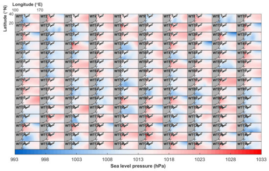
Figure 5.
A total of 150 weather types obtained from SLP fields (hPa) using atmospheric classification.

Figure 6.
Distribution of the significant wave height and the mean wave direction associated with each weather type at THL2B location.
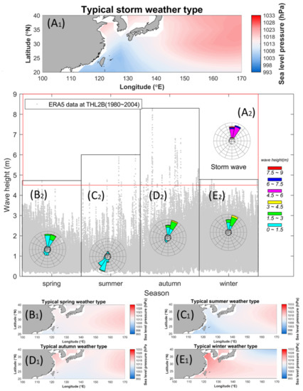
Figure 7.
Relationship between the representative atmospheric patterns corresponding to the wave conditions at the THL2B site. (Different weather types are (A) storm, (B) spring, (C) summer, (D) autumn and (E) winter. Subscripts are (1) weather type pattern and (2) corresponded wave rose diagram).
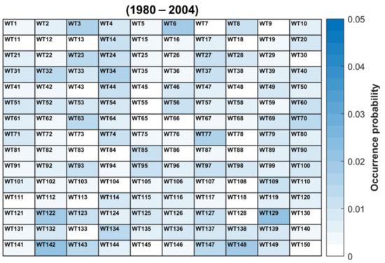
Figure 8.
Occurrence probability of 150 weather types for the reference period from 1980 to 2004.
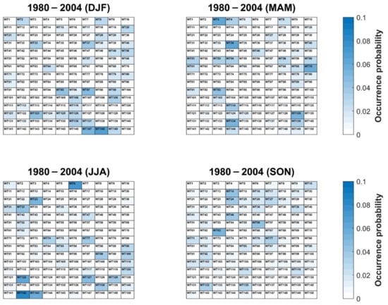
Figure 9.
Seasonal occurrence probability of 150 weather types for the reference period from 1980 to 2004.
Further, the corresponding relationship between Figure 5 and Figure 6 is extended to all grid points around Taiwan (20° N to 27° N and 119° E to 123° E) based on the resolution of ERA5 reanalysis wave data, which can establish the relationship between the predictor and predictand based on and the associated weather types near Taiwan. To verify the SD model, a comparison was made between the statistical downscaling estimation and the significant wave height data from ECMWF, which was validated from 2005 to 2017. The validation uses the monthly mean of to evaluate the results via a correlation coefficient (), estimated:
where and are the variance of the reanalysis data and SD data, respectively. Figure 10 shows the results of the validation, where the spatial domain spans from 20° N to 27° N and 119° E to 123° E. Additionally, owing to the empirical relationship, the spatial resolution is changed from 2.5° by 2.5° to 0.5° by 0.5° through SD. The results for the south and west of Taiwan in the re part are better, with correlation coefficients of 0.78 to 0.90.
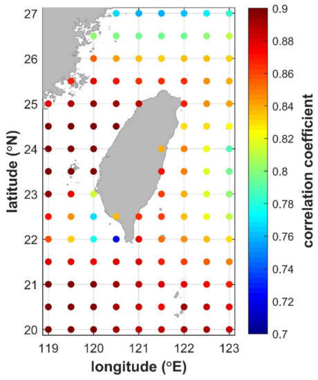
Figure 10.
Results of the validation in terms of correlation coefficients. The spatial domain spans from 20° N to 27° N and 119° E to 123° E.
Figure 11 compares the SD model with the reanalysis data in terms of the monthly mean of at 24° N and 120.25° E, where the best performance was obtained (correlation coefficient of 0.87). The SD model results well reproduce the trend of reanalysis data, but the local maxima in winter show visible deviations. The main reason for these deviations is likely the monsoon climate in Taiwan. In winter, the northeast monsoon has a strong wind intensity, making wind waves dominate and swell in a local region. ESTELA assesses the spatial domain of the predictor based on the generation area of the swell. Under this assumption, the results in the winter are underestimated by the quasi-real data with strong wind waves.
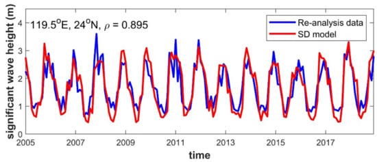
Figure 11.
Comparison of monthly between the quasi-real data and the model at 24° N, 119.5° E in a time series for the validation period from 2005 to 2017. The blue line shows the monthly from the re-analysis data. The red line is the monthly from the proposed downscaling approach. The correlation coefficient is approximately 0.895.
4. Results
4.1. Selection of GCMs
The IPCC provides atmospheric data from GCMs simulated at many national research institutions. These GCMs include some future scenarios under various intensities of greenhouse gas emissions. The most critical problem with GCMs is model uncertainty. The data from GCMs are determined using complicated physical equations that describe atmospheric and ocean dynamics. Therefore, different methods and considerations are used in the simulations to solve these equations and lead to different results, even though they all consider the same radiative forcing values globally. To analyze the accuracy of GCMs, Perez, Menendez [19] proposed a methodology and performance indices. The framework attempts to reproduce a historical synoptic situation. The GCMs were evaluated by comparing the SD model’s outputs and the reanalysis data for a reference period from 1980 to 2004. That period was chosen because the ECMWF data began in 1980, with the most historical GCM simulations ending in 2004. The study uses several GCMs provided by the fifth assessment report (AR5), where future scenarios are represented by multiple representative concentration pathways (RCPs). IPCC describes RCPs in four paths: RCP2.6, RCP4.5, RCP6, and RCP8.5, which are named for their radiative forcing values.
The performance results of the GCMs are shown in Table 1. () is the root-mean-square error normalized by the mean of the historical occurrence probability and is calculated as:
where is the historical occurrence probability for the reference period, is the relative probability from each GCM simulation, and is the number of weather types.

Table 1.
Performance evaluation of 17 GCMs. Eliminated GCMs are marked as (X).
The index compares the similarity between the quasi-real data and each GCM simulation by estimating the sum of the relative difference based on the reanalysis from each weather type for the reference period. The relative entropy is used to analyze the low occurrence probability and is defined as:
where the log term is sensitive because the probability of any GCM is small. This property indicates the lack of a synoptic situation based on the quasi-real data from GCM simulations. Hence, lower values of and represent a high degree of similarity to reality. Additionally, this study also analyzes the variability in the four seasons (, , , and ) and the consistency. Each column’s threshold is defined as the mean value of the index plus one standard deviation [20]. GCM is eliminated if any index exceeds the thresholds. In addition, this study also compared whether the index of each GCM data was consistent within the reference period or not. Use the statistical method of the interquartile range (IQR) as a judgment [19], where and are the first and third quartile ranges, respectively. If the scatter index , determines that the GCM is an outlier, it means that the GCM should not be used and should be removed.
Table 1 shows the initial 17 GCMs and finally reduces them to 10 GCMs. Based on the thresholds mentioned above, GCMs are eliminated and marked in red. The selected GCMs are used to project using the scenarios of RCP4.5 and RCP8.5 and are re-gridded to a 2.5° × 2.5° grid consisting of the predictor. BCC-CSM1.1 has the best performance of the selected GCMs, which means the simulation is similar to the weather type classification predictor for the reference period. The spatial distribution of pressure becomes complicated in summer and autumn because the typhoons that form near Taiwan move through different paths in low-pressure systems. Due to the difference in the grid size for each GCM, the simulations for typhoon events performed similarly. Thus, the values of ( and ) are higher than other indices.
4.2. Future Projection
Scenarios RCP4.5 and RCP8.5 are used for future projection. RCP4.5 is a relatively stable state, whereas RCP 8.5 is a scenario with high emissions of greenhouse gases. First, the projection of a significant wave height near Taiwan for 2020 to 2099 is divided into four periods of 20 years each. Statistical downscaling is applied to the clustering, and the occurrence probability for the variations in the change from the ten selected GCMs, in the short-, mid-, long-term, and end-of-century (2020–2039, 2040–2059, 2060–2079, and 2080–2099), are evaluated with respect to the reference period (1980–2004). Figure 11 shows the rate of change of in RCP4.5 and RCP8.5 for each future period and is evaluated as:
where is the mean of the results from the selected GCMs.
Figure 12 depicts the results of the change rate of around Taiwan for four periods between the RCP4.5 and RCP8.5 scenarios. The spatial minimum, maximum, average, and standard deviation are listed in Table 2. It shows that the change rate of around Taiwan might not be evident from 2020 to 2099, and the change rates of are all less than 1%. Overall, the change of decreases with the increase in the time for both RCP4.5 and RCP8.5. In both scenarios, the maximum increase and decrease of the are shown in the short-term (2020–2039) and the end-of-century (2080–2099), respectively. The maximum increase in the for RCP4.5 and RCP8.5 are 0.84% and 0.44%, respectively. In addition, the maximum decrease of (−0.92%) is shown in the future period (2080–2099) under RCP8.5. On the other hand, the standard deviation shows completely different results at the end-of-century (2080–2099). The change of in the RCP4.5 is uniform, yet nonuniform in the RCP8.5. It should be noted that only minimal changes nearby Taiwan and the value of the wave climatic difference are close to zero, and that is consistent with the ensemble results published by Hemer et al. (2013).
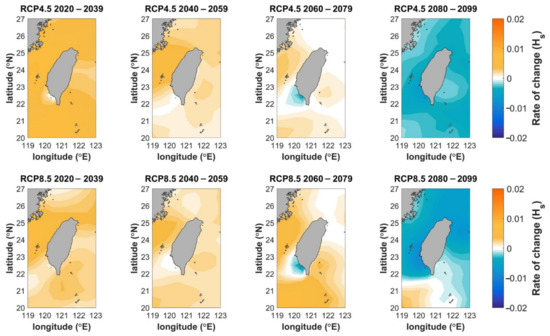
Figure 12.
Rate of change in the annual mean of significant wave height of selected GCMs with respect to the reference period from 1980 to 2004 in the region of Taiwan for various future periods (2020−2039, 2040−2059, 2060−2079, and 2080−2099) and scenarios (RCP4.5 and RCP8.5).

Table 2.
Quantitative assessment of future wave climate change results around Taiwan.
Moreover, to analyze the results of each GCM, Figure 13 shows a box plot for 23.5° N and 120° E. The figure indicates the apparent changes and best results for the validation. Even though there are outliers, consistent performance is observed for other simulations of GCMs.
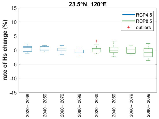
Figure 13.
Box plot of rate of change in the averaged significant wave height for each GCM, with respect to the reference period from 1980 to 2004 in the region of Taiwan at 24° N, 120.15° E for various future periods (2020–2039, 2040–2059, 2060–2079, and 2080–2099) and scenarios (RCP4.5 and RCP8.5).
The resolution depends on the historical database used for the reference. The climate in Taiwan has significant seasonal influence, especially northeast monsoons in winter and typhoons in the summer and autumn. Hence, the seasonal changes are taken into consideration in the current study. The changes in the winter wave climate gradually increase with time for RCP8.5, as depicted in Figure 14, which is more regular than the corresponding change for RCP4.5. The RCP4.5 scenario prediction results in Figure 15 are quite varied across the GCMs, while those for RCP8.5 are relatively consistent. In summer, the changes in the wave climate are more consistent than in the winter, and the trend of the wave climate is mainly incremental in the short-term (2020 to 2039) period and decreases with time, as shown in Figure 16. Figure 17 shows that the divergence in the GCM model prediction results is higher in the summer than in winter (Figure 15), and most GCM results show an incremental trend at the observation site. For autumn, the trend of the wave climate change around Taiwan mainly decreased under the two scenarios and decreased with time. The rate of change for RCP8.5 is faster than that for RPC4.5, as shown in Figure 18. In Figure 19, the values in the fourth period under RCP4.5 and RCP8.5 scenarios significantly decrease for most GCMs at the site 24° N, 120.15° E. Finally, the increment change in the wave climate in spring is the largest, but the trend will decrease with time, as shown in Figure 20. In Figure 21, the median rate of change during short-term period increases is about 4%: the largest among all seasons. A comparison of all the seasons indicates that the trend of wave climate changes in the Taiwan area is mainly incremental in the short-term period and decreases with time. The trends of the simulations are more consistent in the spring and autumn, as shown in Figure 15, Figure 17, Figure 19, and Figure 21. Figure 22 shows the near future (short-term period) climate change trend at location (23.5° N, 120° E). The area with the flat coastal line was affected seriously due to climate change in Taiwan. Additionally, overall, the wave climate conditions show an increasing trend during the short-term period. Seasonally, the wave climate conditions tend to weaken in winter, with the largest increase in spring, followed by summer, while the wave climate change in autumn is not obvious.
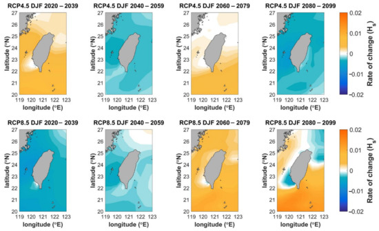
Figure 14.
Rate of change in the seasonal mean of significant wave heights for each GCM, with respect to the reference period from 1980 to 2004 in the region of Taiwan in winter for various future periods (2020–2039, 2040–2059, 2060–2079, and 2080–2099) and scenarios (RCP4.5 and RCP8.5).
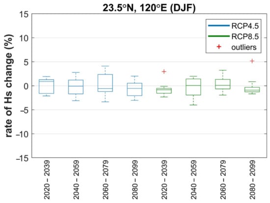
Figure 15.
Box plot of rate of change in the seasonal mean of significant wave heights for each GCM, with respect to the reference period from 1980 to 2004 in the region of Taiwan in winter at 24° N, 120.15° E for various future periods (2020–2039, 2040–2059, 2060–2079, and 2080–2099) and scenarios (RCP4.5).
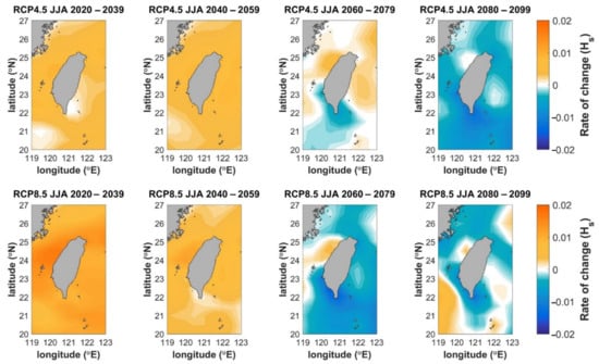
Figure 16.
Rate of change in the seasonal mean of significant wave height for each GCM, with respect to the reference period from 1980 to 2004 in the region of Taiwan in summer for various future periods (2020–2039, 2040–2059, 2060–2079, and 2080–2099) and scenarios (RCP4.5 and RCP8.5).
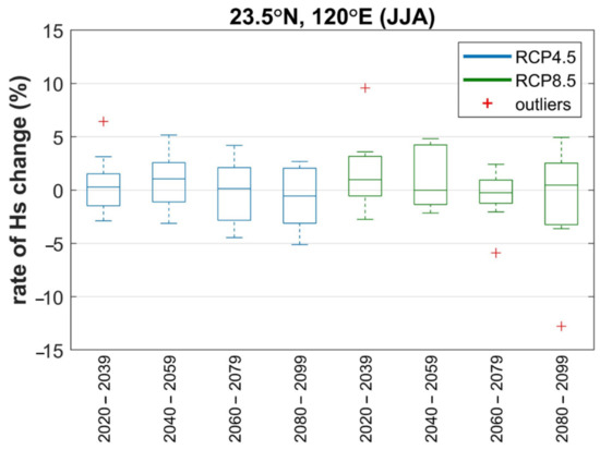
Figure 17.
Box plot of rate of change in the seasonal mean of significant wave heights for each GCM, with respect to the reference period from 1980 to 2004 in the region of Taiwan in summer at 23.5° N, 120° E for various future periods (2020–2039, 2040–2059, 2060–2079, and 2080–2099) and scenarios (RCP4.5 and RCP8.5).
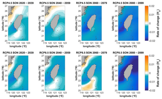
Figure 18.
Rate of change in the seasonal mean of significant wave heights for each GCM, with respect to the reference period from 1980 to 2004 in the region of Taiwan in autumn for various future periods (2020–2039, 2040–2059, 2060–2079, and 2080–2099) and scenarios (RCP4.5 and RCP8.5).
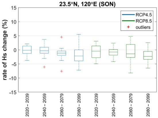
Figure 19.
Box plot of rate of change in the seasonal mean of significant wave heights for each GCM, with respect to the reference period from 1980 to 2004 in the region of Taiwan, in autumn at 23.5° N, 120° E for various future periods (2020–2039, 2040–2059, 2060–2079, and 2080–2099) and scenarios.
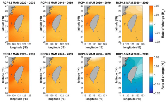
Figure 20.
Rate of change in the seasonal mean of significant wave heights for each GCM, with respect to the reference period from 1980 to 2004 in the region of Taiwan in spring for various future periods (2020–2039, 2040–2059, 2060–2079, and 2080–2099) and scenarios (RCP4.5 and RCP8.5).
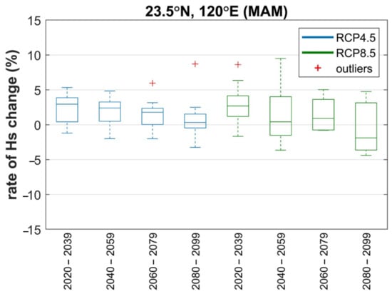
Figure 21.
Box plot of rate of change in the seasonal mean of significant wave heights for each GCM, with respect to the reference period from 1980 to 2004 in the region of Taiwan in spring at 24° N, 120.15° E for various future periods (2020–2039, 2040–2059, 2060–2079, and 2080–2099) and scenarios (RCP4.5 and RCP8.5).
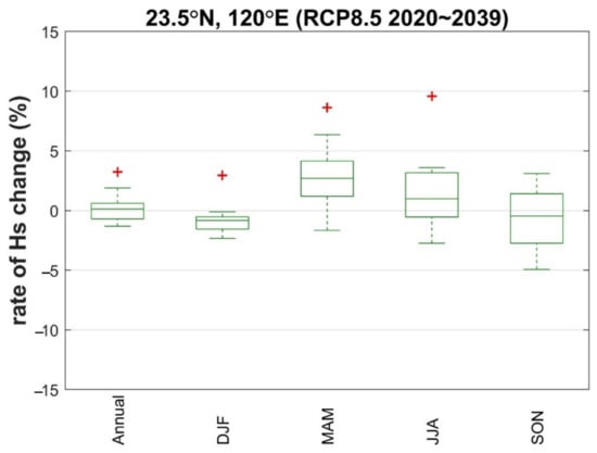
Figure 22.
Box plot of rate of change in the seasonal mean of significant wave heights for each GCM, with respect to the reference period from 1980 to 2004 in the region of Taiwan at 23.5° N, 120° E for various future periods (2020–2039) and scenarios (RCP8.5).
5. Summary and Conclusions
Statistical downscaling is applied to the Taiwan region using a weather-type approach to project the future wave climate. The main advantages of the method are low computational cost and multiple GCM analyses for future projections. Unlike most dynamic simulations, SD projections are not limited to the end of the 21st century, thus providing a temporal coverage of the whole century. Furthermore, the spatial resolution is not fixed, unlike other dynamic simulations; instead, the resolution of the wave height data is significantly increased to 0.5° × 0.5° from atmospheric conditions by applying the weather type SD. This spatial resolution depends on the historical database used for the reference (Camus et al., 2017). In this study, 10 GCMs were selected for the simulation from 2020 to 2099. The results for the rate of wave climate change in the Taiwan region show that there are no specific increasing trends with the increase in climate change, which are similar to those from previous studies (e.g., Hemer et al., 2013; Mori et al., 2010). The main findings of this study are:
- The validation results based on the reference period (1980–2004) are best in the west and south of Taiwan, where the correlation coefficients are up to 0.78–0.90. This difference is caused by the different travel times of the wave energy to local areas and the island shielding effect.
- Although the historical data of GCMs are consistent with each other in the reference period (1980~2004), as shown in Table 1, the future climate change results from GCMs show significant differences. Annual wave climate change does not have a significant relationship with the increase in climate change scenarios. It is speculated that the climate conditions in Taiwan are dominated by the monsoon, and the impact of climate change is only in specific seasons.
- More evident changes are observed due to the monsoon season in Taiwan. Notably, the changes near the west region increase dramatically in the spring.
In our method, there are a number of outliers, including a consistent performance which is observed for other simulations of GCMs and the fact that the spatial resolution was downscaled from 2.5° × 2.5° to 0.5° × 0.5°. This relies on the temporal resolution of the reanalysis data. Increases in the quality of reanalysis data will provide finer resolutions. The validation for data around Spain was reproduced [13] (data not shown), but the validation for Taiwan did not match perfectly. This variation might be due to the more varied climate seasons of Taiwan, such as typhoons and four-season monsoons, in which wind waves dominate the swell. The above shows the diversity of climate patterns in the region, and it explains why more clusters are considered in this area and will obtain better verification results. In the future, we can consider the topographic changes induced by wave climate and associated with weather type, which can be applied to the impact of climate change on coastal erosion and deposition.
Author Contributions
Methodology, S.-C.H., C.-H.T. and W.-S.L.; supervision, S.-C.H. and W.-S.C.; software, W.-S.L. and K.-C.H.; validation, C.-H.T., W.-S.L. and W.-S.C.; data analysis, W.-S.L. and K.-C.H. All authors have read and agreed to the published version of the manuscript.
Funding
This study was financially supported from the National Science and Technology Council, Taiwan (MOST 109-2217-E-006-002-MY3).
Institutional Review Board Statement
Not applicable.
Informed Consent Statement
Not applicable.
Data Availability Statement
Not applicable.
Conflicts of Interest
The authors declare no conflict of interest.
References
- Camus, P.; Losada, I.; Izaguirre, C.; Espejo, A.; Menéndez, M.; Pérez, J. Statistical wave climate projections for coastal impact assessments. Earth’s Future 2017, 5, 918–933. [Google Scholar] [CrossRef]
- Camus, P.; Méndez, F.J.; Losada, I.J.; Menéndez, M.; Espejo, A.; Pérez, J.; Rueda, A.; Guanche, Y. A method for finding the optimal predictor indices for local wave climate conditions. Ocean Dyn. 2014, 64, 1025–1038. [Google Scholar] [CrossRef]
- Camus, P.; Menendez, M.; Mendez, F.J.; Izaguirre, C.; Espejo, A.; Canovas, V.; Perez, J.; Rueda, A.; Losada, I.J.; Medina, R. A weather-type statistical downscaling framework for ocean wave climate. J. Geophys. Res. Ocean. 2014, 119, 7389–7405. [Google Scholar] [CrossRef]
- Chien, H.; Cheng, H.-Y.; Chiou, M.-D. Wave climate variability of Taiwan waters. J. Oceanogr. 2014, 70, 133–152. [Google Scholar] [CrossRef]
- Hastie, T.; Tibshirani, R.; Friedman, J.H.; Friedman, J.H. The Elements of Statistical Learning: Data Mining, Inference, and Prediction; Springer: New York, NY, USA, 2009; Volume 2. [Google Scholar]
- Hegermiller, C.; Antolinez, J.A.; Rueda, A.; Camus, P.; Perez, J.; Erikson, L.H.; Barnard, P.L.; Mendez, F.J. A multimodal wave spectrum–based approach for statistical downscaling of local wave climate. J. Phys. Oceanogr. 2017, 47, 375–386. [Google Scholar] [CrossRef]
- Hemer, M.A.; Fan, Y.; Mori, N.; Semedo, A.; Wang, X.L. Projected changes in wave climate from a multi-model ensemble. Nat. Clim. Change 2013, 3, 471–476. [Google Scholar] [CrossRef]
- Hemer, M.A.; Wang, X.L.; Weisse, R.; Swail, V.R. Advancing wind-waves climate science: The COWCLIP project. Bull. Am. Meteorol. Soc. 2012, 93, 791–796. [Google Scholar] [CrossRef]
- Hsiao, S.-C.; Chiang, W.-S.; Jang, J.-H.; Wu, H.-L.; Lu, W.-S.; Chen, W.-B.; Wu, Y.-T. Flood risk influenced by the compound effect of storm surge and rainfall under climate change for low-lying coastal areas. Sci. Total Environ. 2021, 764, 144439. [Google Scholar] [CrossRef] [PubMed]
- Jolliffe, I.T. Principal Component Analysis for Special Types of Data; Springer: New York, NY, USA, 2002. [Google Scholar]
- Laugel, A.; Menendez, M.; Benoit, M.; Mattarolo, G.; Méndez, F. Wave climate projections along the French coastline: Dynamical versus statistical downscaling methods. Ocean. Model. 2014, 84, 35–50. [Google Scholar] [CrossRef]
- Mori, N.; Yasuda, T.; Mase, H.; Tom, T.; Oku, Y. Projection of extreme wave climate change under global warming. Hydrol. Res. Lett. 2010, 4, 15–19. [Google Scholar] [CrossRef]
- Perez, J.; Mendez, F.J.; Menendez, M.; Losada, I.J. ESTELA: A method for evaluating the source and travel time of the wave energy reaching a local area. Ocean. Dyn. 2014, 64, 1181–1191. [Google Scholar] [CrossRef]
- Perez, J.; Menendez, M.; Camus, P.; Mendez, F.J.; Losada, I.J. Statistical multi-model climate projections of surface ocean waves in Europe. Ocean. Model. 2015, 96, 161–170. [Google Scholar] [CrossRef]
- Perez, J.; Menendez, M.; Mendez, F.J.; Losada, I.J. Evaluating the performance of CMIP3 and CMIP5 global climate models over the north-east Atlantic region. Clim. Dyn. 2014, 43, 2663–2680. [Google Scholar] [CrossRef]
- Rueda, A.; Camus, P.; Méndez, F.J.; Tomás, A.; Luceño, A. An extreme value model for maximum wave heights based on weather types. J. Geophys. Res. Ocean. 2016, 121, 1262–1273. [Google Scholar] [CrossRef]
- Semedo, A.; Weisse, R.; Behrens, A.; Sterl, A.; Bengtsson, L.; Günther, H. Projection of global wave climate change toward the end of the twenty-first century. J. Clim. 2012, 26, 8269–8288. [Google Scholar] [CrossRef]
- Wang, X.L.; Feng, Y.; Swail, V. North Atlantic wave height trends as reconstructed from the 20th century reanalysis. Geophys. Res. Lett. 2012, 39, L18705. [Google Scholar] [CrossRef]
- Wang, X.L.; Feng, Y.; Swail, V.R. Changes in global ocean wave heights as projected using multimodel CMIP5 simulations. Geophys. Res. Lett. 2014, 41, 1026–1034. [Google Scholar] [CrossRef]
- Wang, X.L.; Swail, V.R.; Cox, A. Dynamical versus statistical downscaling methods for ocean wave heights. Int. J. Climatol. J. R. Meteorol. Soc. 2010, 30, 317–332. [Google Scholar] [CrossRef]
Publisher’s Note: MDPI stays neutral with regard to jurisdictional claims in published maps and institutional affiliations. |
© 2022 by the authors. Licensee MDPI, Basel, Switzerland. This article is an open access article distributed under the terms and conditions of the Creative Commons Attribution (CC BY) license (https://creativecommons.org/licenses/by/4.0/).