Imaging of Artificial Bubble Distribution Using a Multi-Sonar Array System

Abstract

Bubble clusters present in seawater can cause acoustic interference and acoustic signal distortion during marine exploration. However, this interference can also be used as an acoustic masking technique, which has significant implications for military purposes. Therefore, characterizing the distribution of bubble clusters in water would allow for the development of anti-detection technologies. In this study, a sea experiment was performed using a multi-sonar array system and a bubble-generating material developed by our research group to obtain acoustic signals from an artificial bubble cluster and characterize its distribution. The acquired acoustic data were preprocessed, and reverse-time migration (RTM) was applied to the dataset. For effective RTM, an envelope waveform was used to decrease computation time and memory requirements. The envelope RTM results could be used to effectively image the distribution characteristics of the artificial bubble clusters. Compared with acoustic Doppler current profiler data, the backscattering strength of the boundary of the imaged artificial bubble cluster was estimated to range between −30 and −20 dB. Therefore, the three-dimensional distribution characteristics of bubble clusters in the open sea can be effectively determined through envelope RTM. Furthermore, the data obtained from this study can be used as a reference for future studies.

1. Introduction

In marine environments, various forms of bubble layers are constantly induced by the wind, ship movement, the activities of living organisms, earthquakes, and other processes. However, these bubble layers can cause acoustic interferences during acoustic signal acquisition for marine surveys. For example, the acoustic signal received by sonar (sound navigation and ranging) equipment is attenuated by bubble clusters, resulting in a sound pressure level below the expected value. Nevertheless, this same principle can be used as a valuable acoustic masking technique. This technique is widely applied to suppress explosive shock waves by blasting them with bubble curtains, as well as to reduce noise from wind farms [1,2]. Additionally, this technique has been widely investigated for military purposes, such as the development of masker emitter belts to reduce the intensity of noise generated from the hull of a surface ship by artificially generating air bubbles from the hull, which protects the hull from an explosive shock wave of external origin [3,4]. Furthermore, this principle can be used as the basis for the development of a propeller air-induced emission (PRAIRIE) system, which artificially generates air bubbles near the propeller to prevent the propagation of noise and reduce the noise of the cavity caused by the rotation of the propeller of the ship, minimize the vibration of the hull, and suppress propeller erosion [5,6]. Therefore, characterizing the acoustic properties and distribution of bubble clusters in water provides a valuable basis for the development of both civil and military technologies.

Previous studies have explored various approaches to characterize the acoustic properties of air bubbles distributed in water [7,8,9,10]. For instance, our research team successfully measured the acoustic properties of artificially created air bubbles using an acoustic Doppler current profiler (ADCP) [10]. However, unlike the measurement of acoustic properties, characterizing the distribution of bubble clusters in a real sea environment is rather challenging. Since the early studies of Johnson and Cooke [11] and Stokes and Deane [12], many researchers have attempted to measure the distribution of bubbles by using optical data. Recently, Park [13] measured the distribution characteristics of bubble clusters by using a high-speed Photron FASTCAM MiniAX50 camera, whereas Bae et al. [10] measured the distribution of bubbles using a phase Doppler particle analyzer (PDPA). However, these optical measurement methods have inherent limitations because they characterize the distribution of a three-dimensional space using two-dimensional data. Medwin and Breitz [14] and Farmer et al. [15] predicted bubble distribution using an acoustic resonator. However, this approach can only feasibly be used to characterize small areas and is therefore not suitable for measuring larger bubble clusters such as those that occur in real-life situations.

Along with the development of computer technology, an increasing number of studies have explored the applicability of numerical analysis techniques for image analysis. Acoustic tomography is a numerical analysis technique that is widely used in geophysics and oceanography. This technique is used to estimate the distribution of objects in a three-dimensional space by determining the point at which the difference between the observed travel time and the value calculated through numerical modeling is minimized. This approach allows researchers to quickly and efficiently characterize the long-wavelength structures of a given medium [16]. Waveform inversion, which is another numerical analysis technique, performs optimization using not only travel time but also a variety of waveform details such as amplitude and phase. In contrast, acoustic tomography uses travel time only. The waveform inversion technique requires the sound source signal used for accurate imaging. Additionally, more accurate property estimation and imaging can be achieved as the number of receivers increases. However, computational cost constitutes another important bottleneck, as these costs increase rapidly as sampling frequency increases [17]. To address this issue, Zhang et al. [18] proposed a source-independent direct envelope inversion (SIDEI) approach and demonstrated that physical properties can be effectively obtained using arbitrary sound source information even without accurate source information. This technique uses a sound source with a lower frequency than that of the source of the observation data and utilizes the envelope of the observed signal. Therefore, robust results can be obtained with a low computational cost. However, despite the many advantages of acoustic tomography and SIDEI for the estimation of the boundary of distribution, these techniques cannot accurately estimate the exact boundary.

Reverse-time migration (RTM) is another numerical analysis technique that can accurately derive information on the interface of a medium. This approach is mainly used to understand the structure of strata and reservoirs in natural resource surveys. RTM has a lower computational cost than other numerical analysis techniques and can be imaged with fewer transmitters and receivers. Therefore, RTM is widely used in geophysics and other fields [19]. The RTM value at a specific point in the grating medium can be accurately estimated through zero-lag cross-correlation between the wavefield radiated by the source and the wavefield reflected from the anomaly [20]. However, modeling the reflected wavefields from the anomaly is challenging. Therefore, once the back-propagated wavefield is obtained by reversely propagating the acoustic signal recorded in the receiver, an accurate boundary can be obtained through zero-lag cross-correlation with the source wavefield. This technique allows for the estimation of the boundary of the medium, but the physical property value cannot be estimated.

In this study, we estimated the three-dimensional distribution characteristics of a bubble cluster in a marine environment by applying RTM. The analysis of three-dimensional characteristics is often time-consuming and demands a high level of computational resources and associated costs. Therefore, an envelope waveform for a sound source with a lower frequency than the actual one was used to overcome this problem. Six sonar array systems with the same configuration were designed and developed to acquire acoustic signals from the bubble cluster and used as measuring devices. After generating the artificial bubbles in the center area of the measuring device installed for the sea experiment, sound waves were transmitted and recorded to obtain the sound waves affected by the artificial bubbles. The acquired acoustic data were then submitted to a simple preprocessing process, after which the RTM technique with the envelope of the waveform was applied to successfully image the distribution of the bubble clusters. Section 2 introduces the RTM with an envelope waveform used for bubble distribution imaging. Section 3 describes the design of the sea experiment, including the composition of the sea experiment, the equipment, and the measurement method. Section 4 explores the applicability of the proposed method through a synthetic example. This section also presents the results derived from imaging the three-dimensional distribution of bubble clusters in an actual sea experiment. Finally, Section 5 summarizes our key findings and conclusions.

2. Imaging Technique for Bubble Distribution

In this study, the RTM method based on the numerical modeling of the acoustic wave equation was applied to image the distributional characteristics of the bubble cluster. In this method, imaging condition $I$ can be derived by determining the zero-lag cross-correlation between the wavefield propagated from the sound source and the wavefield obtained by back-propagating the observation data recorded in the receiver [21].

$$I\left(x,y,z\right)={{\displaystyle \int }}_0^{t_{max}}{P}_s\left(t,x,y,z\right)P_r\left(t_{max}-t,x,y,z\right)dt$$

(1)

Here, $x,y,\mathrm{and} z$ are the three-dimensional positions, $t$ is the time, $P_s$ is the forward propagated wavefield of the source, $P_r$ is the back-propagated wavefield from the receiver, and $t_{max}$ is the maximum recording time. This amplitude provides no explicit physical relationship such as reflectivity. However, it does provide a boundary structure, because this method is meant to accurately detect the location of the boundary where the sound waves are reflected due to differences in acoustic impedance [22]. In this study, an envelope waveform was used to reduce computational cost. If Equation (1) is expressed as the zero-lag cross-correlation between the observation data expressed by the envelope waveform and the partial derivative wavefield, it can be expressed as Equation (2) [20,23]:

$$I\left(x,y,z\right)={{\displaystyle \int }}_0^{t_{max}}{\left[\frac{\partial E_u\left(t\right)}{\partial m\left(x,y,z\right)}\right]}^T{E}_d\left(t\right)dt,$$

(2)

where $m$ is the sound velocity; $E_u$ is the envelope of signals generated by numerical modeling; $E_d$ is the envelope of signals obtained from the real experiment; operator $T$ is the transpose matrix. The partial derivative wavefield of the sound velocity at each point in the envelope of the modeling data is expressed in the following equation as a direct envelope Fréchet derivative based on the energy-scattering method [24,25]:

$$F_E=\frac{\partial E}{\partial m}=G_0^{\left(e\right)}{Q}_0^{\left(e\right)},$$

(3)

where $G_0^{\left(e\right)}$ is Green’s function of the envelope and $Q_0^{\left(e\right)}$ is the virtual source of the envelope waveform. The final RTM expression using the envelope waveform can be derived by substituting Equation (3) into Equation (2) as follows:

$$I\left(x,y,z\right)={{\displaystyle \int }}_0^{t_{max}}{Q}_0^{\left(e\right)}\left(t,x,y,z\right)\left[{{\displaystyle \int }}_0^{t_{max}}{G}_0^{\left(e\right)}\left(\phi -t\right)E_d\left(\phi \right)d\phi \right]dt$$

(4)

Forward modeling is conducted, and the virtual sound source term can be derived by calculating the envelope of the obtained wavefield. Then, the back-propagated wavefield is obtained by calculating the wavefield at all of the points after the envelope of the observed data is back-propagated at the receiver points. The distribution boundary of the bubble layer can be imaged by cross-correlating the obtained back-propagated wavefield with the envelope virtual source term. Accordingly, this method can be used to image the distribution characteristics of the bubble cluster. Additional bubble-distribution-related features, such as the survival time and distribution depth of the bubble cluster, can be estimated by observing the changes in the bubble cluster over time.

3. Design of the Sea Experiment

3.1. Experiment Configuration

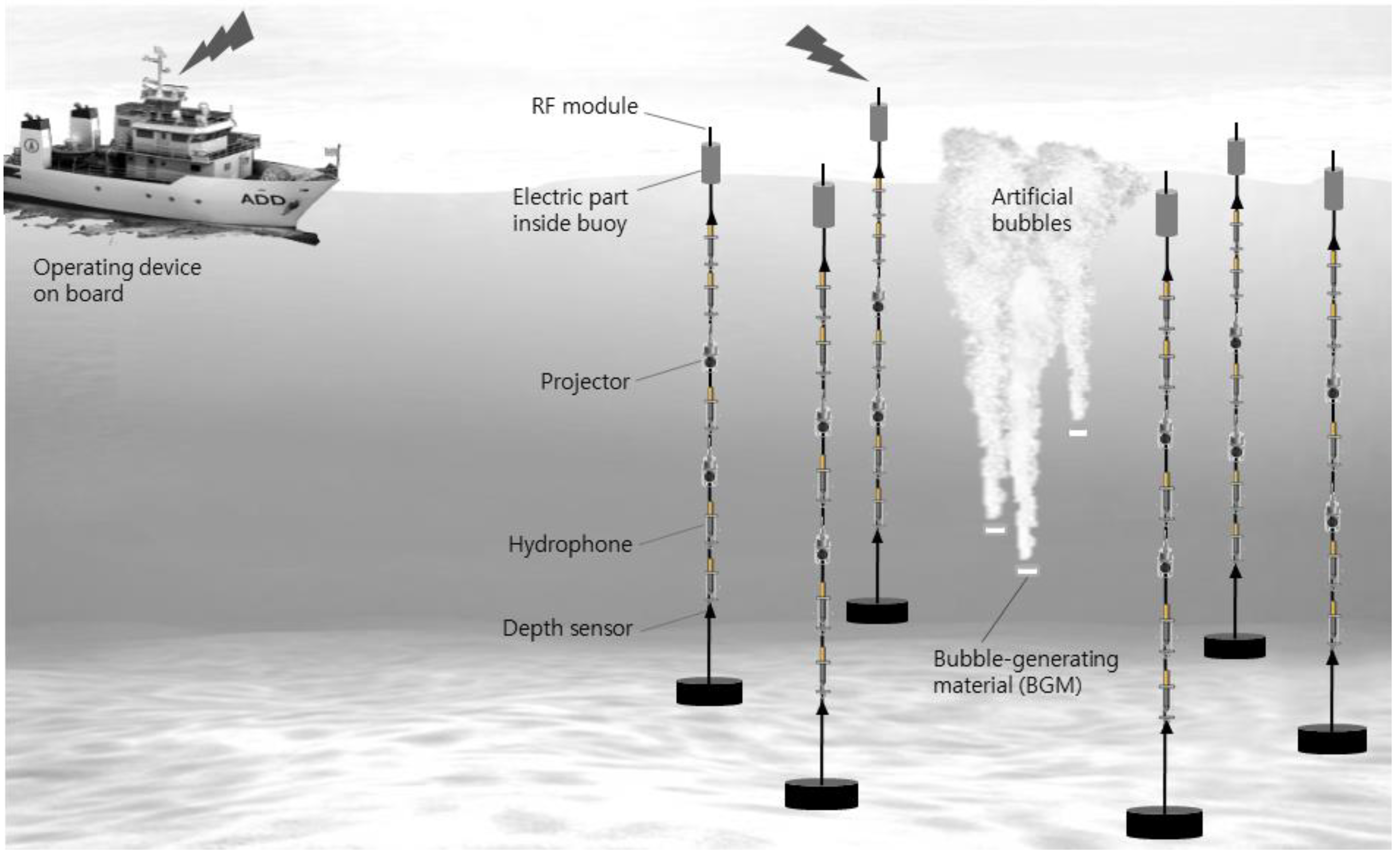
Reflected or scattered acoustic signals must be acquired from bubble clusters to confirm their distribution in a seawater environment. In this study, a suitable sonar array system was developed to successfully acquire the acoustic signal for the bubble cluster. Figure 1 illustrates a schematic of the sea experiment that was conducted to obtain acoustic data using a multi-sonar array system. In the experimental design, sonar arrays, including transmitters and receivers, are deployed to have a certain distance from the bubble cluster to be measured. The main control unit that controls the six sonar array systems is located on a survey ship, and a radio frequency (RF) modem is used to communicate with the sonar array system. An acoustic source is transmitted by a measurement system to the water based on the signals received from the RF modem. A radiated acoustic signal is then passed or reflected by the bubble cluster and recorded by receivers located in the measurement system. The recorded data are transmitted to a survey vessel through RF communication so that an operator can monitor the cluster in real time. The transmitters and receivers of each measurement system are synchronized using a GPS module. Additionally, the exact depth of each sensor can be monitored using the depth sensors located at the top and bottom of each system array.

3.2. Development of a Measurement System

A measurement system was developed to characterize the distribution of the bubble clusters in the sea. The developed system was composed of six sets of marine buoys and a land station that acquires, displays, and stores the data measured from the buoys in real time.

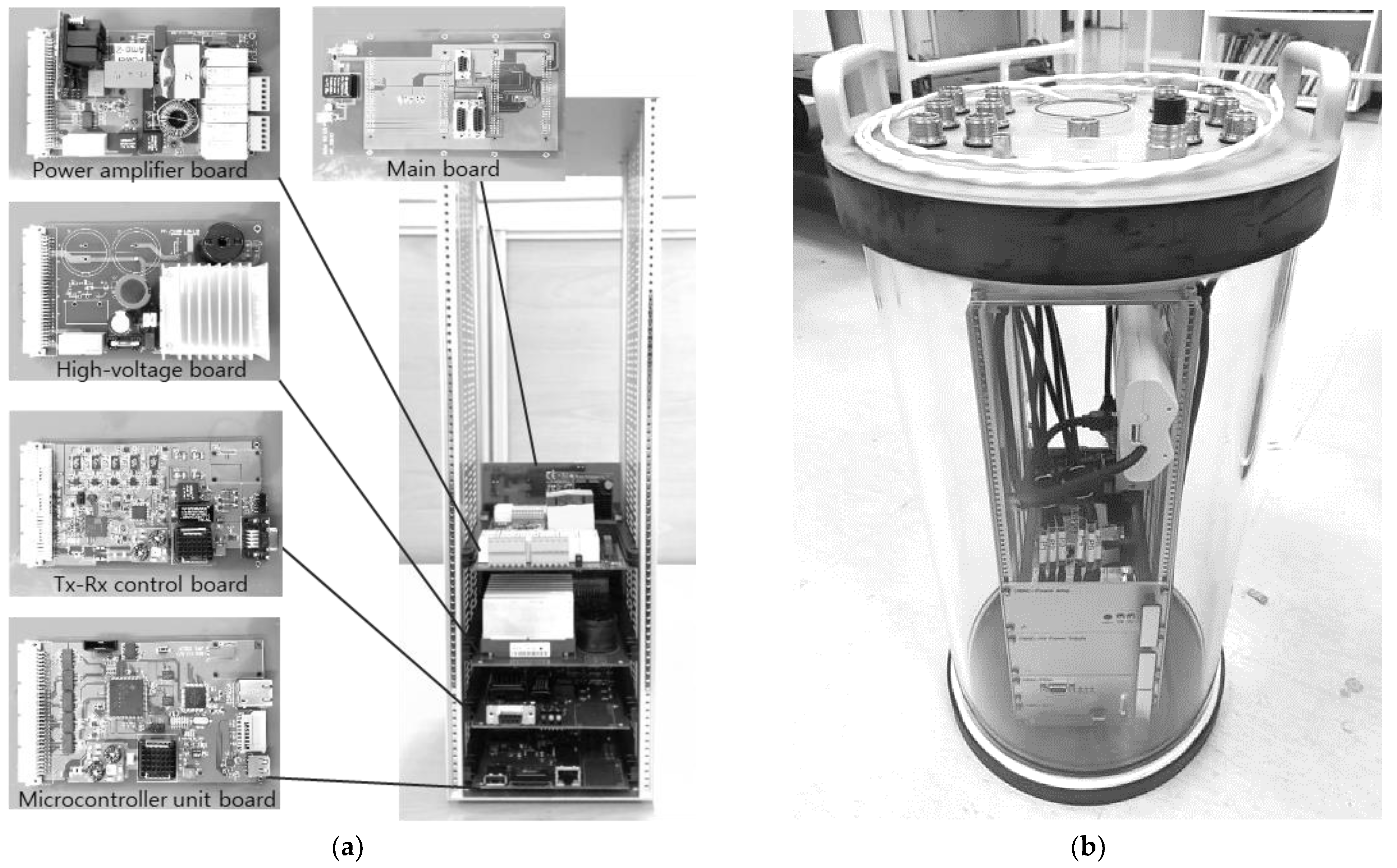
In this system, the marine buoy component transmits sound sources to water according to the command received from the land station, receives the signal reflected from the bubble cluster, and transmits data to the land station. This part consisted of a power amplifier board for an output of >190 dB, a high-voltage board as a power supply, a Tx-Rx control board for signal acquisition and transmission signal generation, a microcontroller unit (MCU) board, and the main board (Figure 2). Additionally, an RF communication modem was mounted on the system to link to the land station. The marine buoy component was a combination of two projectors (Teledyne Marine TC 1026), five hydrophones (Benthowave BII-7016FG), two pressure depth sensors, a GPS module, an RF communication antenna, and a buoy containing electronic components. 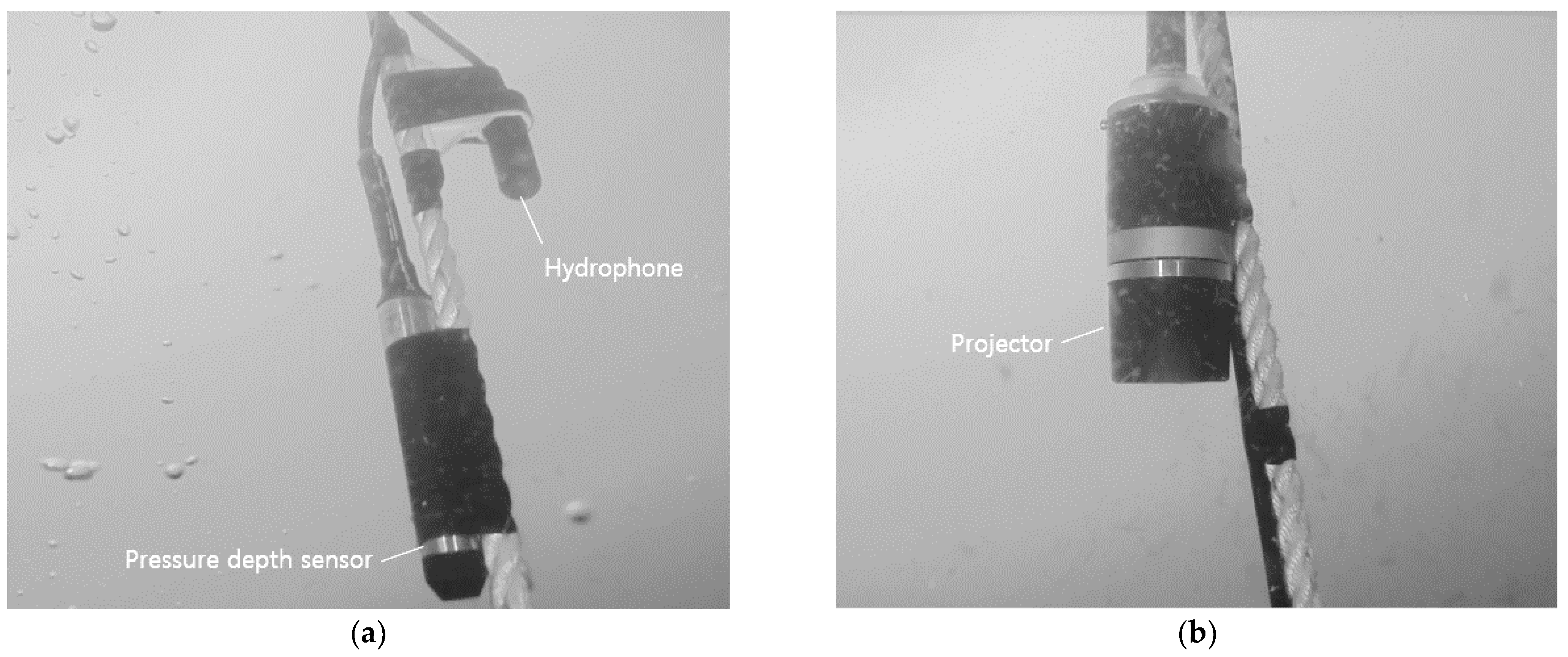Figure 3a shows the receiver sensor (hydrophone) and pressure depth sensor mounted on the system array, and Figure 3b illustrates the transmission sensor (projector) in the system array. The marine buoy component was deployed on a circumference with a radius of approximately 20 m, and acoustic sources were sequentially transmitted from 12 transmitters according to the start command received through RF communication. The system continuously synchronizes with a time error of ≤40 µs from the GPS information until a stop command is received. Furthermore, the protocol was configured so that the land station could verify whether the marine buoy is operating normally. The dynamic range of the measurement system was designed to satisfy ≥80 dB by considering the reflectivity of the bubble cluster, and the sampling rate was set at 120 kHz by considering the frequency of the transmission signal.

The land station sends a command to the marine buoy parts and stores the measurement data received from the marine buoy component. The land station was designed as a standalone PC with an Intel i7-1165G7 CPU and 16 GB of RAM for data collection. Additionally, an RF communication antenna was installed to communicate with the marine buoy component. For in situ quality control of the received signal, a user interface was developed for the operator.

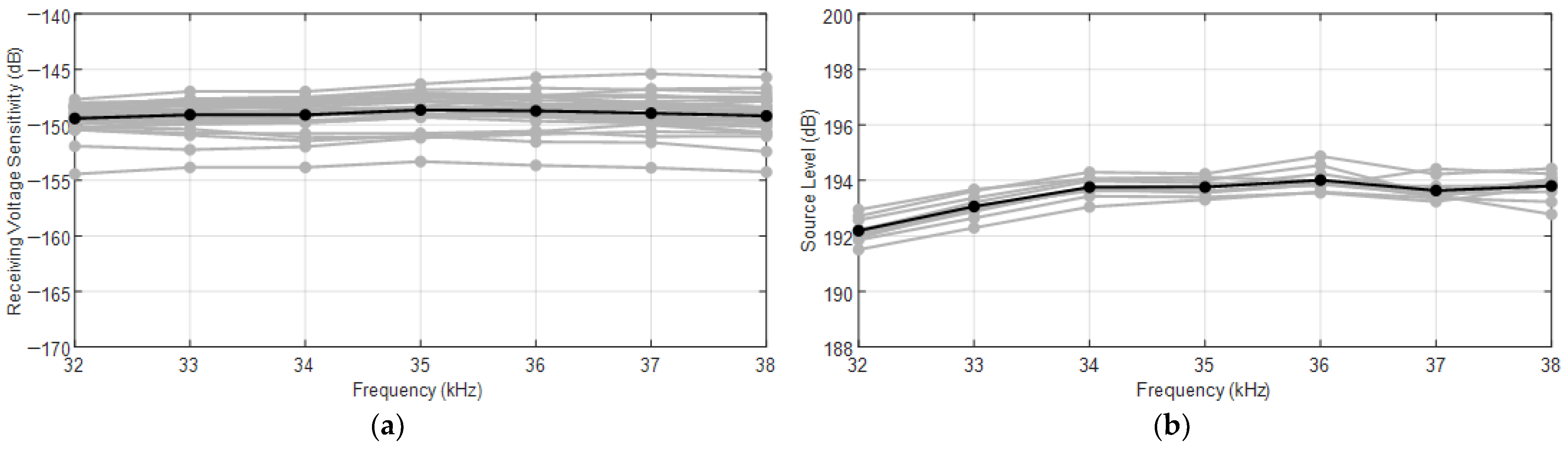
The receiving voltage sensitivities of the hydrophones and the source pressure levels of the projectors were measured in advance in an indoor water tank to confirm the performance of the acoustic sensors used in the measurement system and secure the correction data for the acoustic data. The receiving voltage sensitivities of the 30 hydrophones used in this experiment are shown with gray solid lines in Figure 4a, where the black solid line indicates the mean values. The average receiving voltage sensitivity was −149 dB re 1 V/$\mathsf{\mu }$pa in the center frequency band, and the difference in the sensitivity of the sensor with the largest deviation was approximately 4.8 dB. The source levels of the projectors are presented in Figure 4b, where the mean value of 193.6 dB re 1$\mathsf{\mu }$pa/V in the central frequency band is indicated by black dots with a black solid line, showing a difference of 0.78 dB from the sensor with the largest deviation. These results were later used to correct the amplitude of the received signals. Additionally, the responses of the frequency filter for the receiving amplifier, gain control, and crosstalk were within the design value range. Collectively, these observations validated the reliability of the developed system.

3.3. Artificial Bubble Generation

The bubble clusters measured in this study were generated using a material that generates bubbles through a chemical reaction upon contact with water, which we developed in a previous study. When developing this material, one of our priorities was to ensure that the material was harmless to the marine ecosystem. The bubble-generating material (BGM) used in this experiment was also introduced in our previous research [10]. The BGM was precisely dropped into the center of the observation area by using a drone to avoid interfering with other acoustic signals such as radiation noise and reflection signals from the ship.

3.4. Data Measurement

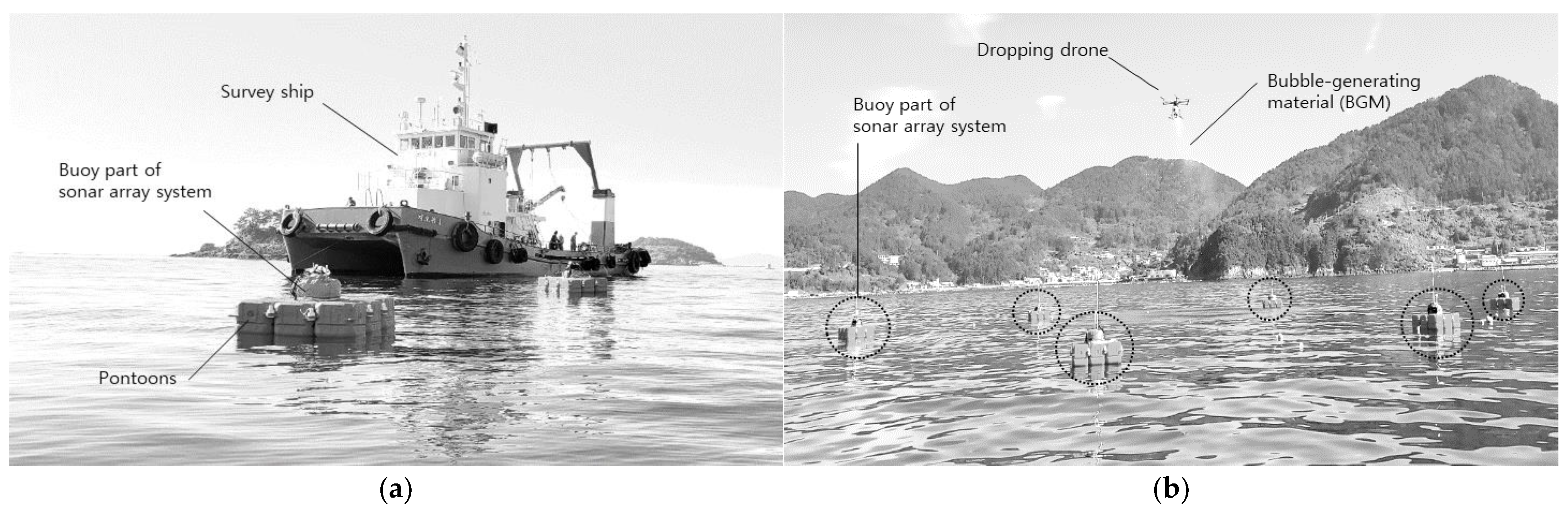
An acoustic measurement experiment was performed in November 2021 at the time of the tidal tide, when water flow is the slowest in the southern seas of the Korean Peninsula. The deployment of the marine buoy components is shown in Figure 5a. The buoys were stably installed in the sea using eight pontoons around the buoys, which contain the electronic components. Six sets of measurement buoys were installed in a circle with a radius of 20 m at intervals of 60° to estimate the three-dimensional distribution of the bubble cluster.

The receiving sensors in the array were positioned at intervals of 2 m from a depth of 2–10 m, which was the expected distribution depth of the bubble cluster, and the transmitting sensors were positioned at 5 and 7 m. When a command for measurement was transmitted from the land station to the marine buoy components through RF communication, 12 transmitting sensors in the six sets of the measurement buoys sequentially radiated sound sources. The sound sources were designed to be as short as possible within the range where the signal could be perceived to minimize interference between signals. For this purpose, a signal in the form of a sinusoidal wave with a length of 10 wavelengths was used for the acoustic wavelet, and the pulse repetition interval (PRI) was set at 0.5 s. Therefore, all transmissions could be completed in 6 s (6 s/cycle).

Once the measurement system was confirmed to be operating normally, a drone was used to drop the BGM into the target area. During the drop, an actuator and a rotating plate were used to ensure that the BGM had an appropriate drop density to ensure that it landed evenly on the sea surface to generate sufficient bubble clusters. Figure 5b illustrates an example of an experimental BGM dropping and the acoustic measurements. Acoustic signals emitted from 12 transmitting sensors passed through or reflected the bubble cluster in the water, after which they were recorded in 30 receiving sensors (360 ray paths). The acquired acoustic data were transmitted to the land station through RF communication, and this process was monitored in real time by an operator on the ship. An example of acoustic data obtained through the sea experiment is shown in Figure 6, which illustrates the signal with the bubble cluster (black) in comparison with the signal without the bubble cluster (gray). As illustrated in the graph, the strong scattering signal from the bubbles was recorded between 20 and 35 ms. A total of 41,040 sound signals (360 ray paths × 114 cycles) were obtained. Changes in bubble distribution and survival time with time were analyzed by continuously observing the reflected and scattering signals for the bubble cluster from the acquired signal.

3.5. Data Preprocessing

Noises such as electrical, mechanical, and ambient noises must be suppressed to successfully estimate the distribution of bubble clusters generated by the BGM. Finite impulse response-based band-pass filtering is mainly applied to suppress noises out of the frequency band of the source. This approach is stable and efficient, but some of the frequency band components are lost, resulting in ringing artifacts. However, a Butterworth filter, which is an infinite impulse response filter, generates a minimal phase shift while the cutoff frequency remains constant for all filter orders. In this study, ambient, electrical, and mechanical noises were suppressed using a Butterworth filter during preprocessing.

Although the wave height was low and the wind was calm ($\le 1 \mathrm{m}/\mathrm{s})$ during the sea experiment, some of the acquired data were lost during data transmission through RF communication. If an imaging technique such as RTM is applied to the data with loss, the imaging result may be distorted. In turn, this limits the quantitative analysis of the bubble cluster distribution as a function of time. Liu and Sacchi [26] proposed a method to solve this problem caused by data loss. This scheme quantitatively normalizes the signals by considering the continuity between the lost signal and the near-normal signal.

$$J=\Vert \mathrm{A}{E}_d^{’}-E_d\Vert {}^2+{ϵ}^2\Vert \nabla E_d^{’}\Vert {}^2$$

(5)

In Equation (5), $J$ is the cost function of regularization, $A$ is the sampling operator, $E_d^{’}$ represents the restored data, $ϵ$ is the trade-off parameter, and $\nabla$ is the spatial second derivative operator. The trade-off parameter $ϵ$ is the dominant variable in data restoration, and as its value increases, the continuity of the generated signal improves; conversely, the discrepancy from the original data increases. 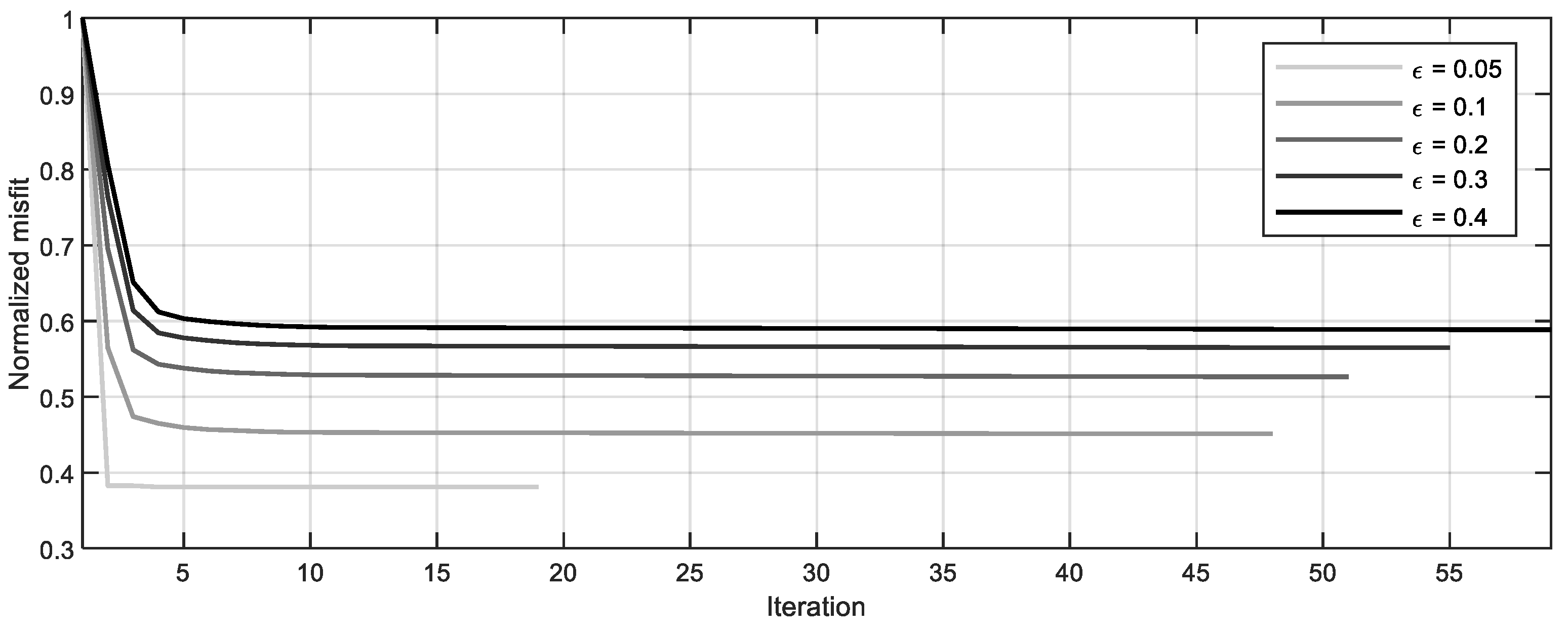Figure 7 shows the misfit curves according to $ϵ$. In each condition, the misfit curve sufficiently converged to the minimum value, and the iterative update was stopped when the misfit difference between the current step and the previous step was within 0.1%. In the graph, when the value of $ϵ$ is low, the error is also low, and the convergence speed is fast. However, in this case, the effect of restoring the lost data was reduced.

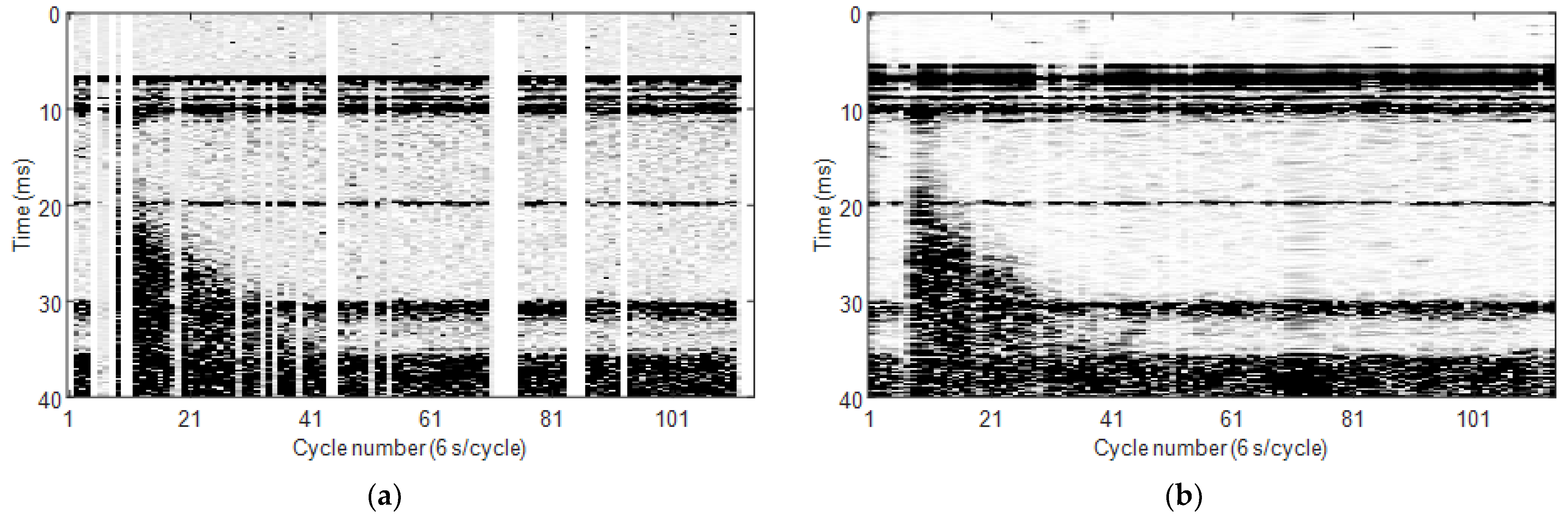
In this study, $ϵ$ was set to 0.1 to account for the data restoration and error occurrence. Figure 8 compares the actual measured raw data with the results after preprocessing. This cycle–time section illustrates the collection of signals recorded by the first receiver (2 m in depth) of the same buoy component from the signal transmitted by the first transmitter (5 m in depth) of the second buoy component. The horizontal axis represents the cycle number (i.e., the number of transmissions), with each cycle being 6 s long. The vertical axis represents the recording time for each transmission signal. After the backscattering signal from the bubble cluster is recognized in the 10th cycle, the signals are identified continuously for 30 cycles (180 s) until the 40th cycle. The signal loss and the background noise are significant in the raw data in Figure 8a, whereas the signal-to-noise ratio (SNR) and data continuity are improved in the preprocessing result in Figure 8b.

4. Results

4.1. Synthetic Data Application

Before the RTM with an envelope waveform was applied to the real data obtained from the sea experiment, the applicability of the proposed method was confirmed by applying it to synthetic data. Figure 9a shows the true sound speed structure of the medium for the generation of synthetic acoustic data. In this structure, the artificial bubble cluster is shaped as a cylinder with a diameter of 6 m and a height of 8 m. The sound speed of the cylinder was randomly distributed within a 1400–1500 m/s range using the “Mersenne twister” random number generator, whereas the sound speed of the background without the bubble cluster was approximately 1500 m/s. The scattering and reflection signals for the bubble cluster were recorded using six measuring buoy systems equipped with two transmitting sensors and five receiving sensors to create the same arrangement of transmitting and receiving acoustic sensors as that in the sea experiment. The solid black circles represent the transmitting sensors, whereas the open circles represent the receiving sensors.

The grid and sampling intervals were determined by considering the dispersion and stability conditions to obtain reliable synthetic acoustic data by minimizing the numerical modeling error [27]. The grid interval in all three axes was set to 0.2 m, and the sampling interval was set to 25 μs. The acoustic observation data for the true sound speed structure in Figure 9a were generated using the Ricker wavelet with a center frequency of 250 Hz as a source, which is indicated by a solid black line in Figure 10. Here, a finite difference was applied for numerical modeling based on the acoustic wave equation, and numerical modeling was performed considering a perfectly matched layer for boundary conditions [28,29].

To image the distribution of the bubble cluster in three dimensions, we individually calculated the envelope virtual sound source term through forward modeling, as described in Equation (4), and the back-propagated wavefield term using observation data. As mentioned earlier, three-dimensional numerical analysis demands a considerable amount of computation time and memory. In this study, an envelope waveform with a frequency lower than the actual frequency was applied to overcome this problem. The validity of this technique should be verified before application. In this process, each envelope wavelet was calculated by performing forward modeling based on a constant velocity model (1500 m/s) with the Ricker wavelet of 250 Hz (black solid line in Figure 10) as a true source and the first derivative of the Gaussian wavelet of 160 Hz (gray solid line in Figure 10) as an alternative source. Figure 10 shows the difference between the two waveforms in the time domain and the frequency domain. Additionally, back-propagation wavefield terms at all positions were derived by back-propagating the enveloped observation data at all receiver positions in the constant velocity model. The boundary was imaged by cross-correlating the envelope virtual sound source and the back-propagated wavefield.

Figure 9b shows the three-dimensional distribution of the bubble clusters derived through envelope RTM when the modeling source and the observation data source are the same as the 250 Hz Ricker wavelet. Figure 9c presents the result obtained by using the first derivative of the Gaussian wavelet of 160 Hz as the modeling source, which has a lower frequency and a different waveform than the observation data source. The two results are similar, and the cylindrical bubble cluster was well imaged. For a more detailed comparison of the two results, we analyzed two-dimensional cross-sections indicated by the gray slice cross-sections in Figure 9c. Figure 11a shows the X–Y section at Z = 4 m, Figure 11b illustrates the X–Z section at Y = 0 m, and Figure 11c presents the Y–Z section at X = 5 m. In comparison with the bubble boundary in the true sound speed structure represented by the gray dashed line, the result (solid black line) clearly showed the bubble cluster boundary when the source of observation and modeling is a Ricker wavelet of 250 Hz, even though a small number of sensor arrays were used. Furthermore, when another waveform (first derivative of the Gaussian wavelet) with 160 Hz was used as the source (gray solid line), the boundary of the bubble cluster was accurately estimated. A similar result to the one achieved using the same source can be obtained using the source with a different waveform having a lower frequency than that of the source of the observation data with a lower computational cost. Therefore, we concluded that our approach is effective and robust.

The RTM technique using the envelope waveform was validated by applying it to the synthetic data; thus, the distribution of the bubble cluster could be estimated. Accordingly, we sought to estimate the three-dimensional distribution of the artificial bubble cluster generated from the BGM by applying it to the data obtained through the sea experiment.

4.2. Artificial Bubble Estimation Using Envelope RTM

The distribution characteristics of the bubble cluster artificially generated in the sea area were imaged using the envelope RTM technique. As previously described in Section 3, after the BGM was dropped onto the sea surface via a drone, the acoustic signals for the bubble cluster were acquired from a multi-sonar array system. Forward modeling was performed for the inheritance (1500 m/s) model by using a 700 Hz Ricker wavelet as a source, whose frequency was lower than that of the source used in the sea experiment, to calculate the wavefield. Afterward, the envelope virtual sound source was obtained by taking the envelope along the time axis. The back-propagated wavefield was calculated by back-propagating the observation data that took the envelope in the same way as in the synthetic data application. Finally, a bubble distribution image was obtained by cross-correlating the back-propagated wavefield with the envelope virtual sound source.

Figure 12 shows the change in bubble distribution over time with the position measured by GPS on the measuring buoys. The figure also presents the bubble cluster imaging results estimated by the envelope RTM technique in cycles #10 (60 s), #17 (102 s), #27 (162 s), and #37 (222 s). In cycle #10 of Figure 12a, bubble clusters were not yet strongly developed. However, in cycle #17 of Figure 12b, the bubble clusters were strongly generated by biasing toward the center and the direction of buoys 4, 5, and 6. In cycle #27 of Figure 12c, numerous bubble clusters were distributed near buoys 4, 5, and 6, as in cycle #17. However, in cycle #37 of Figure 12d, the bubble cluster disappeared. The analysis of the results of all cycles showed that the bubble cluster was maintained after strong development for more than 180 s and then slowly disappeared. These results were similar to the duration of the scattering signal caused by the artificial bubbles, which was approximately 30 cycles (180 s), as shown in the cycle–time section of Figure 8.

Figure 13 shows the cross-sectional views of the bubble cluster in cycle #27, where artificial bubbles were strongly developed. The cross-sections are the positions where the bubble cluster is most strongly developed, and they are indicated by the gray slice cross-sections in Figure 12c. Figure 13a illustrates the X–Y section at Z = 2 m, Figure 13b shows the X–Z section at Y = −4 m, and Figure 13c presents the Y–Z section at X = −7 m. The distribution characteristics of the artificial bubbles in measurement cycle #27 (162 s) indicate that the artificial air bubbles are strongly developed by biasing toward buoys 4, 5, and 6, as seen in the cross-section at a depth of 2 m. These distributional characteristics imply that the artificial bubble clusters are generated by biases in the corresponding direction due to the influence of wind and water currents when the BGM was dropped by the drone. Additionally, Figure 13b,c shows that the development depth of the artificial bubble clusters in the real marine environment occurred within roughly 4 m.

4.3. Quantitative Approach for Artificial Bubble Boundary

The envelope RTM approach can be used to accurately identify the boundaries of the artificial bubble clusters. However, they are not a specific physical quantity. Therefore, these values were inferred from the measurements obtained by the other equipment to acquire meaningful quantitative values for the boundary obtained through the envelope RTM for the artificial bubble cluster.

In our previous studies, we effectively measured the backscattering strength of the artificial bubbles using ADCP (i.e., a commercial sonar device). In the present study, the same approach as in the previous study was used to quantitatively assess the results of envelope RTM. Specifically, the backscattering strength of the artificial bubbles was applied to determine the distribution of artificial bubble clusters [10]. In Figure 13a, X represents the deployment position of ADCP during the sea experiment, and the area steered by four convex beams is indicated by the dashed lines. Figure 14 shows the backscattering strength of the artificial bubble cluster obtained using the ADCP measurement data at the time of acquiring the data for the envelope RTM result. In Figure 14, the backscattering strength of the artificial bubble cluster was classified from −50 to −20 dB at 10 dB intervals. When the backscattering strength is $\ge$−30 dB, the development depth of the artificial bubble cluster is less than 5 m, and the duration time is approximately 200 s. When the backscattering strength is $\ge$−20 dB, the development depth is 2.5 m or less, and the duration time is roughly 150 s. Through these results, the backscattering strength for the artificial bubble cluster identified from the envelope RTM can be estimated. The backscattering strength of the boundary of the artificial bubble cluster for a development depth of 4 m (Figure 13b,c) and a duration time of 180 s (Figure 12) was confirmed through the envelope RTM ranging from −30 dB to −20 dB.

5. Conclusions

In this study, the envelope RTM approach was applied to determine the three-dimensional distribution characteristics of a bubble cluster artificially generated in a real seawater environment. A sonar array measurement system consisting of six sets of buoys was used to obtain the data. A sea experiment was designed and performed using the developed measurement system and the BGM for artificial bubble generation to obtain the acoustic reflection and scattering signals of the artificial bubble cluster near the Korean Peninsula. Preprocessing analyses including frequency filtering and regularization were applied to improve the SNR of the data.

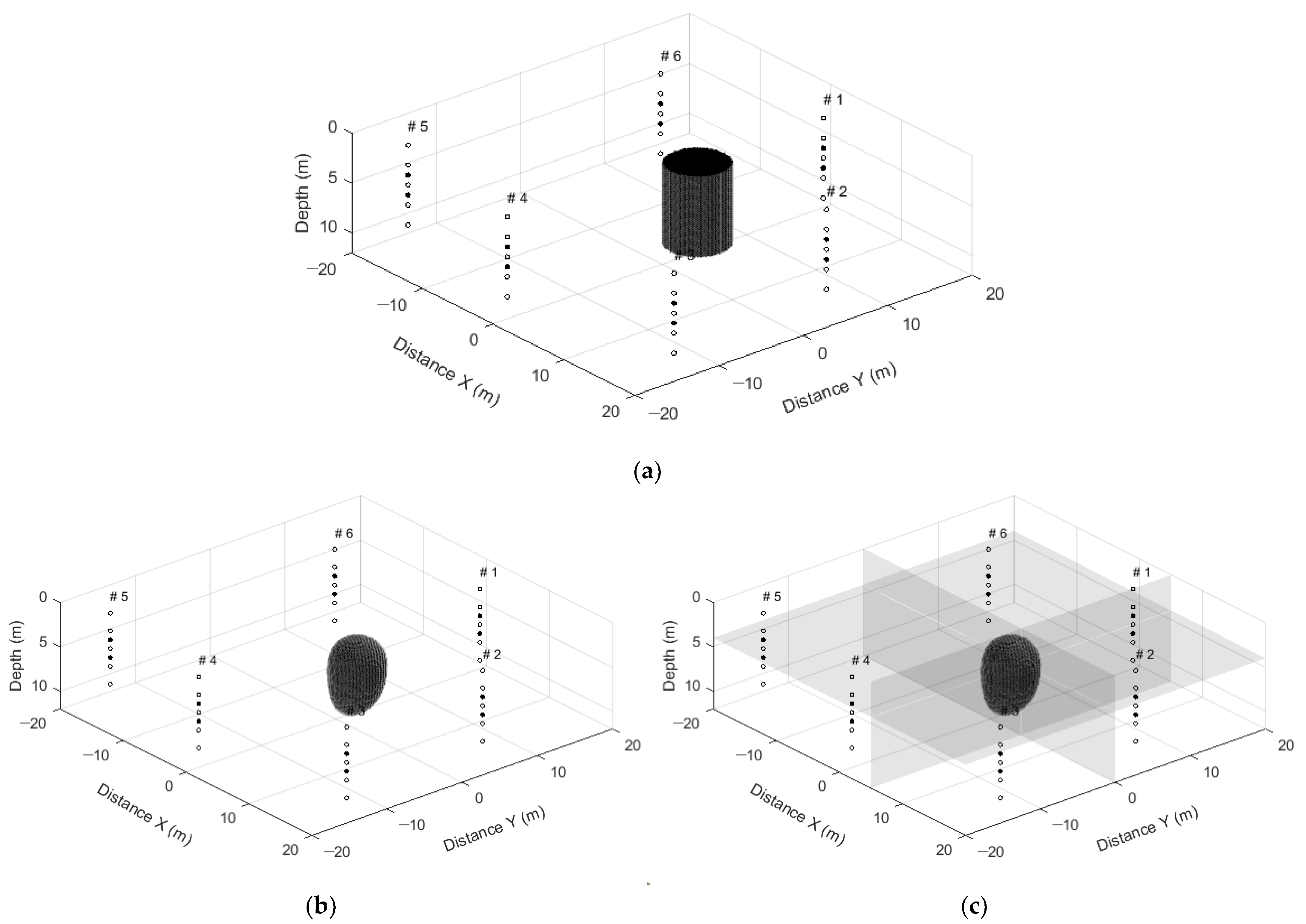
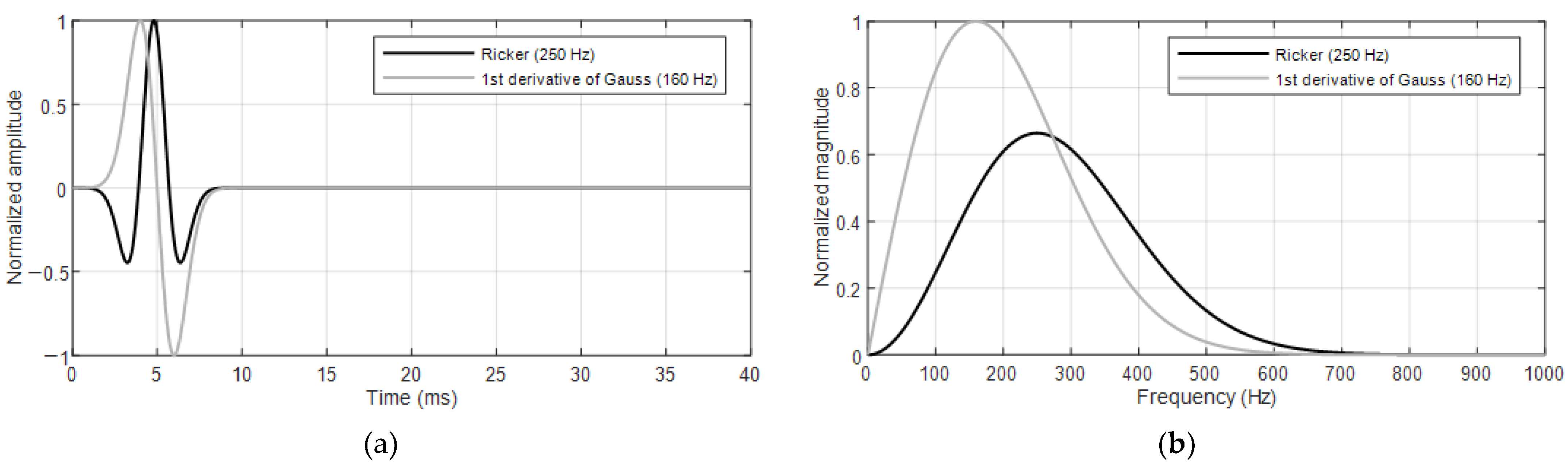
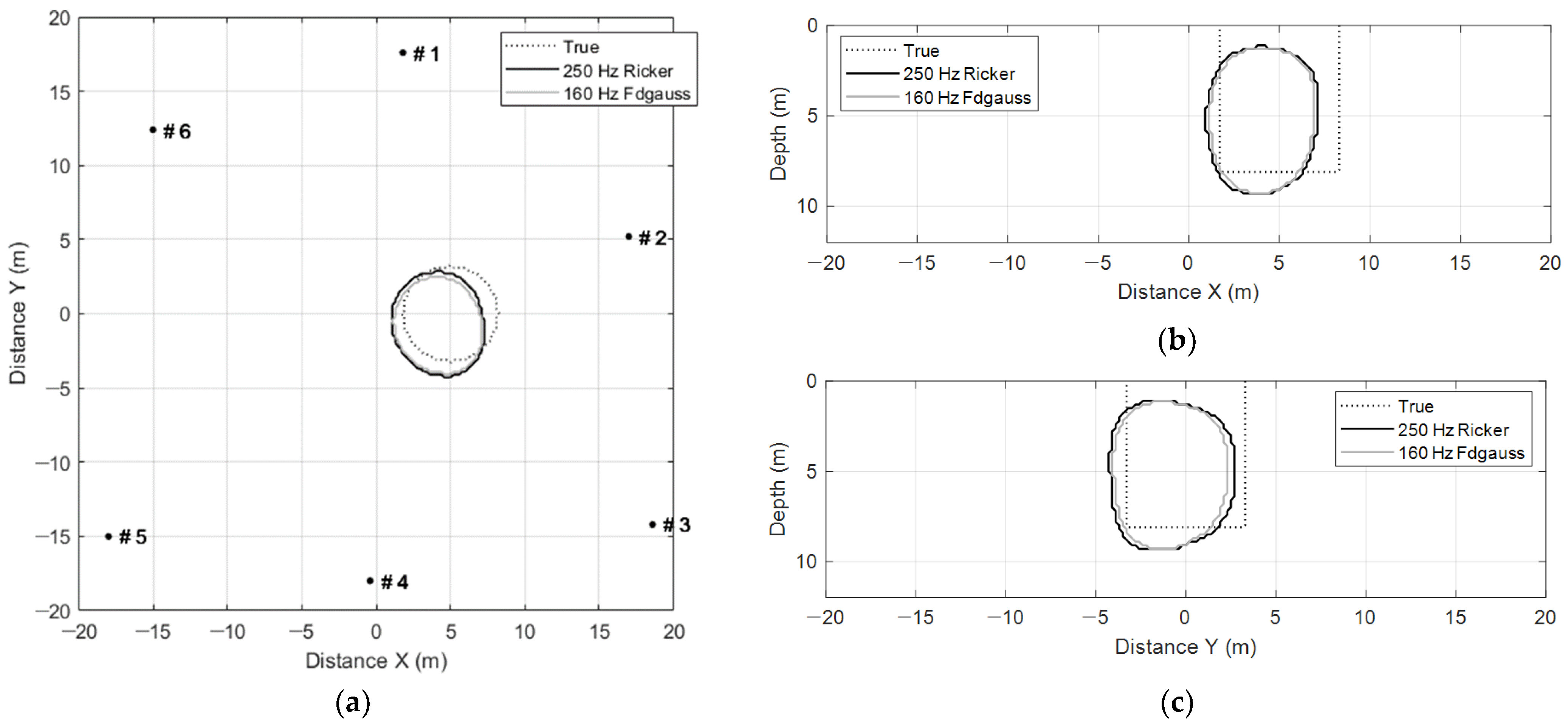
Envelope RTM was applied to the synthetic acoustic data before it was applied to marine experimental data to confirm its validity. The results showed that the boundary of the artificial bubble cluster was effectively derived from a small number of transmitters and receivers. Additionally, the boundary imaging result of the artificial bubble cluster was robust even though we used other waveforms with a lower frequency than the frequency of the source used to generate the observation data.

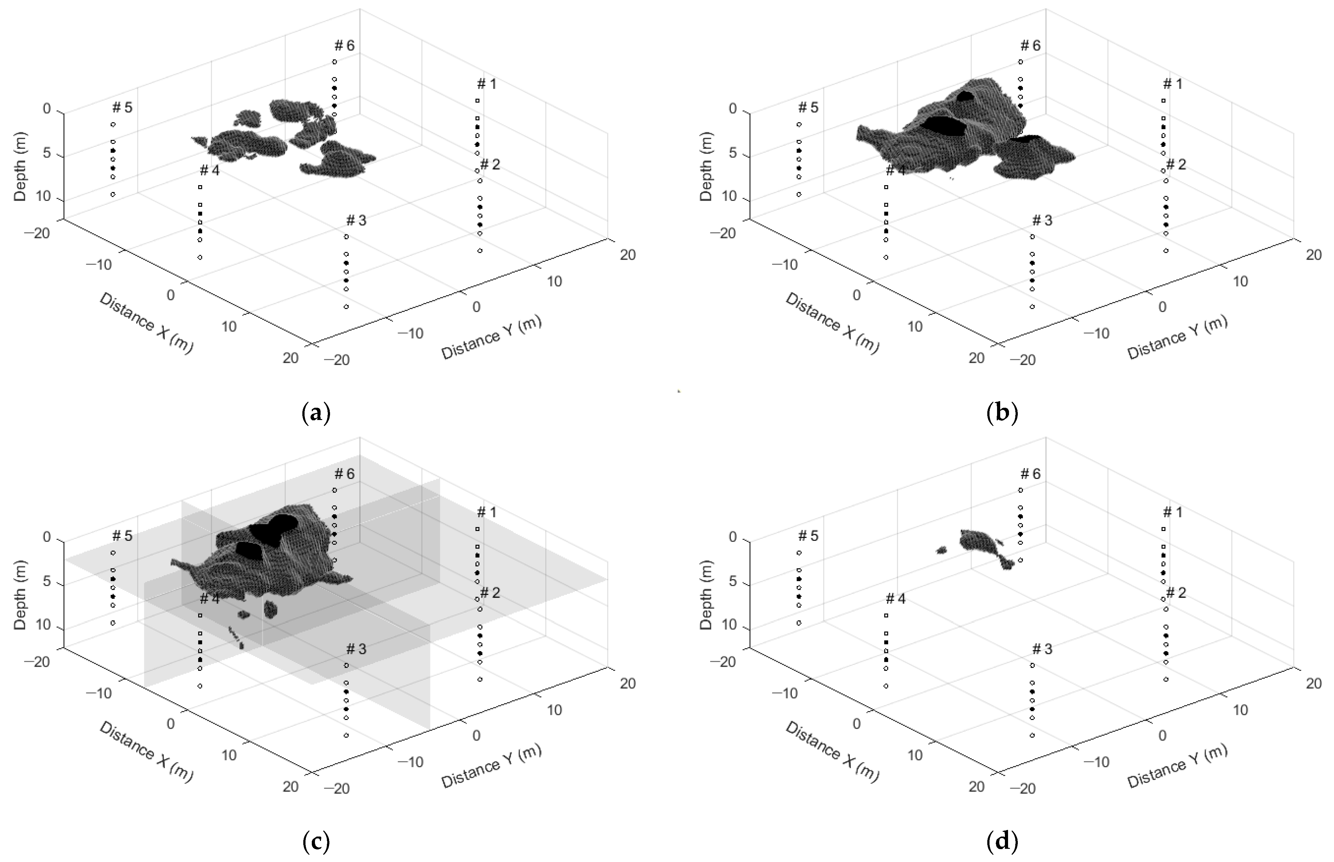
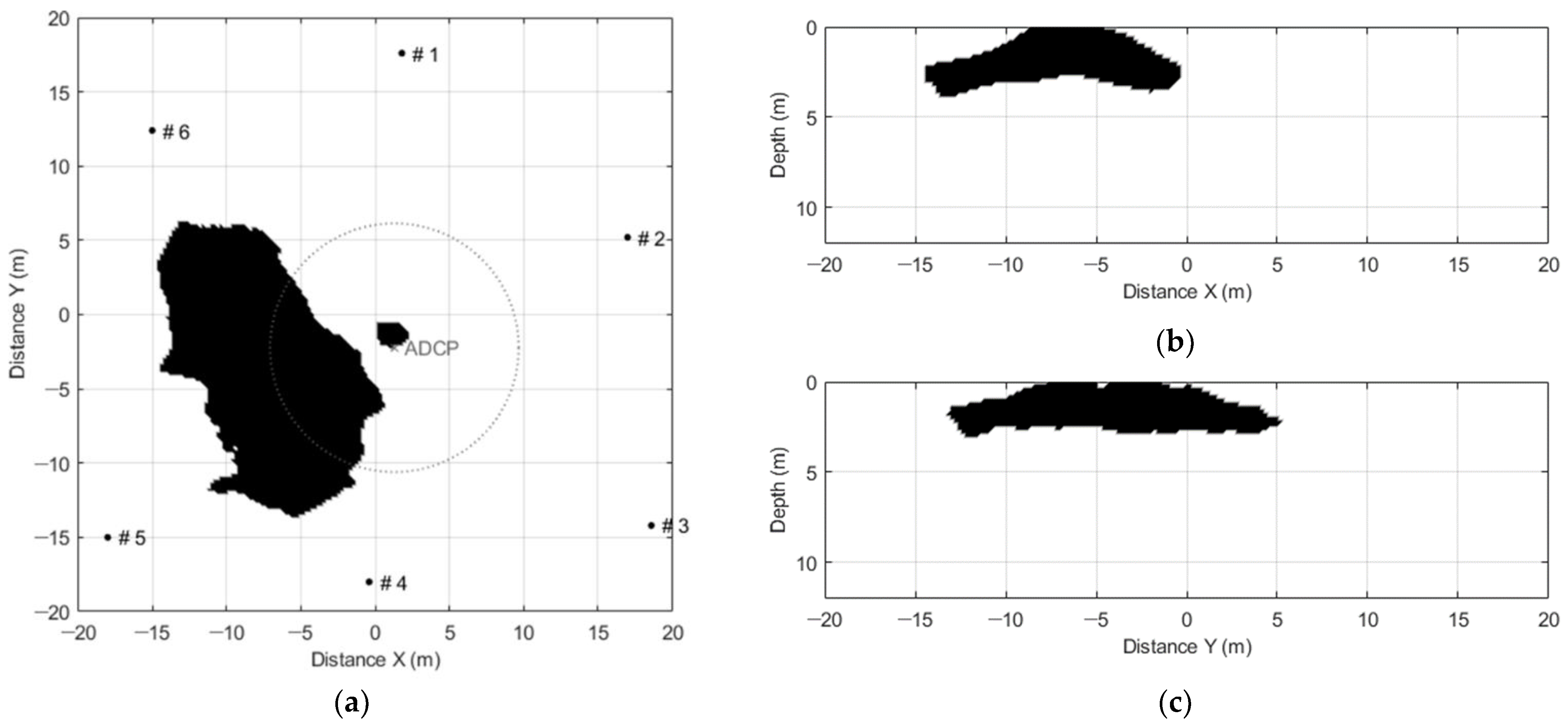
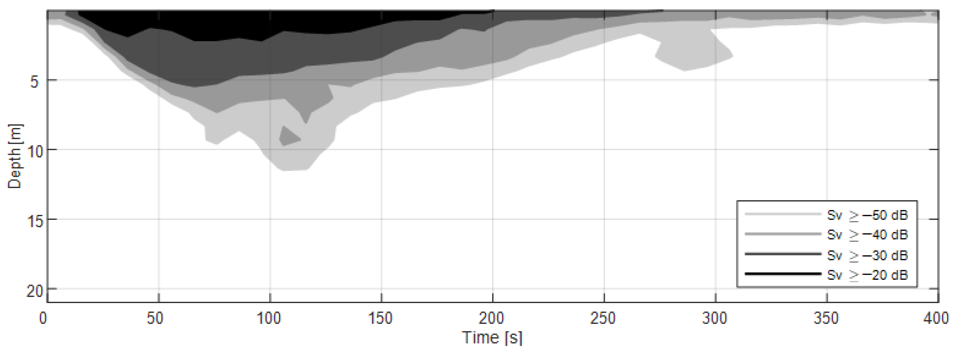
The envelope RTM method verified through synthetic data application was applied to the observed data acquired from the sea experiment. The result demonstrated that the artificial bubble cluster developed and remained strong for more than 180 s in the marine environment, after which it slowly disappeared. The development depth of the artificial bubble cluster was confirmed to be within an approximately 4 m depth. The backscattering strength of the boundary of the artificial bubble cluster imaged through the envelope RTM ranged between −30 and −20 dB in comparison with that of the ADCP data.

Quantitative analysis using marine data is quite limited because the marine environment has a large spatiotemporal variability. In this study, the quantitative analysis of bubble distribution was nearly impossible because the bubble distribution characteristics changed continuously, even during the experiment. Therefore, the quantitative analysis of the bubble distribution presented in this study had some uncertainties. However, the three-dimensional imaging of the bubble cluster in the seawater environment is available, and the reliable boundary of the bubble cluster can be identified through our proposed technique. Therefore, the technique proposed herein can be used to analyze the characteristics of air bubbles present in seawater for both civil and military purposes. Additionally, the distribution characteristics of the artificial bubble clusters estimated in this study can be used as an input value to assess the accuracy of future models focusing on military applications.