Abstract
The cover and management factor (C/B factor) in the Universal Soil Loss Equation (USLE) series models indicates the effects of vegetation cover and management practices on water erosion. Remote sensing technology provides abundant data and methods for the C/B factor estimation, but the applicability and accuracy of these methods can vary widely. More critically, they often overlook the impact of non-photosynthetic vegetation cover on soil erosion. This study aimed to evaluate and develop a more accurate and cost-effective method for calculating the C/B factor in the purple soil hilly region, focusing on typical small watersheds. A correlation analysis was conducted to compare four C/B factors derived from the remote sensing data, aiming to identify the most suitable method for the purple soil hilly region. Additionally, artificial rainfall simulation tests were performed to investigate the relationship between photosynthetic vegetation cover, non-photosynthetic vegetation cover, and soil erosion, leading to the development of a relational equation between integrated vegetation cover and C/B factors. The results indicate that the method from the technical regulations for dynamic monitoring of soil erosion is most suitable for calculating the C/B factor in purple soil hilly regions. On this basis, the integrated vegetation cover effectively accounted for the impact of non-photosynthetic vegetation on soil erosion, leading to a more comprehensive and precise estimation of the C/B factor. The newly developed method significantly improved the accuracy of the C/B factor calculation in the purple soil hilly region. This study provides a scientific and accurate algorithm for calculating the C/B factor in the purple soil hilly region, offering valuable insights and a methodological framework for similar studies in other areas.
1. Introduction
The phenomenon of soil erosion has become a significant global issue, posing serious challenges to the sustainable development of human society [1,2]. Soil erosion assessment is the basis for the accurate identification of soil hazards. Soil erosion assessment methods vary depending on the scale of the study area [3,4]. For large-scale study areas, the factors affecting soil erosion are highly spatially variable; thus, empirical models are mostly used for soil erosion assessment [5,6,7,8,9]. The most well-known of these models is the Universal Soil Loss Equation (USLE), developed by W.H. Wischmeier and D.D. Smith. Since the introduction of the USLE, researchers from various countries have created a series of derived models, such as the Revised Universal Soil Loss Equation (RUSLE) and the Chinese Soil Loss Equation (CSLE) [10,11]. These models usually consist of the rainfall erosivity factor R, the soil erodibility factor K, the slope length factor L, the slope gradient factor S, the cover and management factor C, and the soil and water conservation measure factor P. In the CSLE, the factors C and P are further subdivided into the vegetation cover and biological measure factor B, the engineering measure factor E, and the tillage measure factor T, with the factors C and B both reflecting the role of vegetation cover on soil erosion [12,13,14]. Previous studies have shown that, among these factors, the cover and management factor (C/B) is one of the most spatiotemporally sensitive as it follows plant growth and rainfall dynamics [15]. Therefore, the selection of an appropriate C/B factor calculation method is an important prerequisite for the accurate estimation of soil erosion.
There are several commonly used methods to calculate the C/B factor. One is to refer to the literature and combine it with field observations to correct the assigned value [16,17,18,19]. This method is based on the runoff plot tests conducted by previous scholars to define the factor [18,20,21,22,23]. The method has been the subject of significant recognition in academic discourse. However, the necessity for extensive, long-term runoff plot observations has been identified as a key limitation, resulting in a paucity of data on the C/B factor values calculated using the method. Therefore, using remote sensing to calculate the C/B factor through the normalized vegetation index (NDVI) and other indexes is another commonly used method [24,25]. Through an analysis of the collected and organized literature, the most widely used C/B factor calculation methods include the B calculation method from the technical regulations for dynamic monitoring of soil erosion (Dynamic Monitoring-B), the Cai Chongfa calculation method (Cai-C), the Van calculation method (Van-C), and the Colman calculation method (Colman-C) [26,27,28]. These methods require fewer parameters and simple formulas to obtain the full domain C/B factor of the study area, while the accuracy of the results calculated using these methods is satisfactory. However, the different calculation methods originate from distinct study areas, and the parameters in each method are determined based on the natural characteristics of their respective origin study areas. As a result, the calculation accuracy of these methods varies significantly across different study areas.
It is worth noting that, in nature, vegetation can be divided into photosynthetic vegetation and non-photosynthetic vegetation, according to the functional perspective. Photosynthetic vegetation mainly refers to green vegetation, while non-photosynthetic vegetation includes apoptosis, crop residues, dead leaves, dead branches and stems, and so on [29,30]. At present, when calculating the C/B factor, the base parameter is usually the NDVI, which is based on the strong absorption of vegetation chlorophyll at 690 nm and realizes the quantitative expression of the vegetation state through the combination of the reflectance of the red light and near-infrared bands [31]. Therefore, the vegetation cover calculated using the NDVI refers to the cover of photosynthetic vegetation, while the current methods for calculating the C/B factor value overwhelmingly ignore the effect of non-photosynthetic vegetation cover on soil erosion. The ecophysical status of vegetation is not essential to the erosion process, and non-photosynthetic vegetation as well as photosynthetic vegetation provide a protective layer for the soil [32]. It not only retains rainfall but also absorbs and blocks surface runoff, thus regulating soil moisture and realizing the role of soil and water conservation [33,34,35]. However, in the current application of remote sensing techniques to calculate the C/B factor, the impact of non-photosynthetic vegetation on soil erosion is often overlooked.
Therefore, in this study, in response to the problem of the limited generalizability of remote sensing methods across different regions and the current situation of not considering non-photosynthetic vegetation when calculating the C/B factor, our research employed a two-phase methodology. Initially, we evaluated four widely used C/B factor calculation methods within our study area and selected the most suitable method by correlation analysis. Subsequently, we refined the chosen method by integrating data from artificial rainfall experiments, with a particular focus on accounting for non-photosynthetic vegetation. The primary objective of this study was to identify the most appropriate method for calculating the C/B factor in the purple soil hilly region. Additionally, we aimed to refine this method to improve the accuracy of C/B factor calculations and soil erosion assessments in this region. The second objective was to develop a replicable strategy for screening and enhancing C/B factors that could be applied to related research.
2. Materials and Methods
2.1. Study Area
As a principal tributary in the mid-Jialing River system, the Lizixi watershed (425 km²) occupies a representative purple soil hilly zone within the Sichuan Basin’s central region in China. Its geospatial coordinates span 30°22′–30°42′ N latitude and 105°47′–106°06′ E longitude, with the control station precisely positioned at 30°32′44.002″ N, 105°59′15″ E (Figure 1). This area experiences a humid subtropical climate characterized by distinct seasonal variations, featuring a mean annual temperature of 17.4 °C and substantial precipitation. Topographically, the basin exhibits rolling terrain with elevation gradients from 222 to 503 m, displaying a north-to-south descending profile. Pedologically, the region predominantly comprises purple soils, while land use patterns reveal dryland cultivation (36.70% coverage) and forested areas (31.33%) as the dominant landscape features. Such biophysical attributes collectively establish this watershed as a typological model for studying purple soil ecosystems in subtropical hilly regions [36].
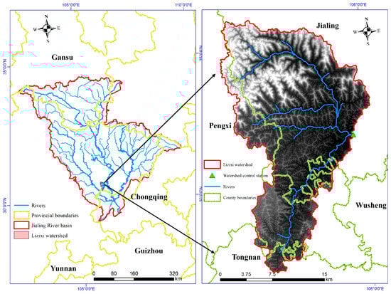
Figure 1.
Location of Lizixi watershed.
2.2. Methods
2.2.1. C/B Factor Calculation
- (1)
- Dynamic Monitoring-B [37]
This method calculates the B factor according to different land use types. If the land use type is cultivated land, construction land, transportation land, water area, water conservancy facility land, or other land, the value is assigned directly to the corresponding land parcel according to regulations. When the land use type is forest land, gardens, or grassland, the calculation formula of the B factor is
where is the ratio of rainfall erosivity calculated in the ith half-month to the annual erosivity, and the value range is 0–1; and is the proportion of soil loss in forest land, gardens, or grassland in the ith half-month, dimensionless, and the value range is 0–1.
The calculation formula for tea gardens and shrubland is
The calculation formula for orchards, other garden land, forest land, and other forest land is
The calculation formula for grassland is
where FVC is the fractional vegetation cover calculated using the parameter correction method based on the MOSIS NDVI data in the past three years, with a value range of 0–1; and GD is the understory coverage of arbor forest, with a value range of 0–1.
- (2)
- Cai-C [26]
The method of calculating is an equation established by Cai in the Three Gorges Reservoir area based on the artificial rainfall and partial natural rainfall data in the runoff plot. The expression is
When applying this method, c can be used as the annual average fractional vegetation cover, monthly average fractional vegetation cover, and seasonal average fractional vegetation cover to calculate the value.
- (3)
- Van-C [38]
The method of calculating is different from the above two methods. The above two methods need to calculate the vegetation coverage based on the NDVI, while the method of calculating directly establishes the equation of the NDVI and C factor value. The basic form is
where the NDVI is the Normalized Difference Vegetation Index and α and β are parameters related to the shape of the curve that associates the NDVI with the factor value, where α = 2 and β = 1.
- (4)
- Colman-C [28]
Similar to the method of calculating , the basic form of this method is also an equation directly established by the NDVI and the C factor value, and its basic form is
where the NDVI is the Normalized Difference Vegetation Index.
2.2.2. Soil Erosion Calculations
To more accurately assess soil erosion, combining the characteristics of Chinese topography and soil and water conservation practices, Chinese scholars have proposed the Chinese Soil Loss Equation (CSLE), which is improved by the USLE and the RUSLE [39,40]. This equation has been used in the national water conservancy census and dynamic monitoring of soil erosion to estimate regional soil erosion after accumulating rich research results [41,42,43,44,45]. The basic form of the equation is as follows:
where A is the amount of soil loss (t·hm−2a−1); R is the rainfall erosivity (MJ·hm−2·mm·h−1·a−1); K is the soil erodibility (t·hm2·MJ−1·hm−2·mm−1·h); L is the slope length factor (dimensionless); S is the slope factor (dimensionless); B is the biological control factor (dimensionless); E is the engineering control factor (dimensionless); and T is the tillage factor (dimensionless). The specific calculation method of each factor and related data sources refer to the previous literature [36].
A = R·K·L·S·B·E·T
2.2.3. Artificial Rainfall Simulation Experiment
Artificial rainfall simulation experiments were conducted in the Three Gorges Reservoir Area Soil and Water Conservation and Environmental Research Station. The selected runoff plot had a concrete bottom and surrounding concrete construction, with dimensions of 8 m × 2 m, a slope of 15°, and a soil thickness of 60 cm. The rainfall equipment used was a BX-1 portable field rainfall device, with a nozzle configuration in the form of a single-spray, double-side arrangement. The rainfall intensity was set at 60 mm/h, and 8 rain barrels were used to ensure rainfall uniformity > 85% and rain intensity deviation < 5%. In this experiment, the vegetation types were mainly alfalfa and alternanthera philoxeroides. According to the classification of vegetation function, the runoff plots of photosynthetic and non-photosynthetic vegetation with different vegetation coverage were laid out, in which the photosynthetic vegetation was the alfalfa and alternanthera philoxeroides during the period of green freshness, and the non-photosynthetic vegetation was the alfalfa and alternanthera philoxeroides after wilting and decaying. The specific deployment requirements involved evenly dividing the runoff plots into 10 strips along the broad side, with each strip being 0.2 m wide. To simulate different coverage levels, 0, 2, 4, 6, 8, and 10 strips were assigned to represent coverage of 0%, 20%, 40%, 60%, 80%, and 100%, respectively. A schematic diagram is shown in Figure 2, and the photo method was used to calibrate the degree of vegetation coverage after the deployment. In this study, each rainfall lasted 40 min. The rainfall calendar time was measured from the onset of runoff production. After runoff began, the sand production was low during the first 10 min but increased rapidly. To accurately capture the original slope sand production process, runoff samples were taken every minute, with each sample having a volume of 200 mL. Due to variations in the rate of sand production under different experimental conditions, the number of samples collected in the first 10 min was not fixed. During the remaining 30 min, the sand production process changed slowly, so samples were taken every 2 min. The number of samples varied with the rate of sand production. Meanwhile, the remaining water–sand samples from each rainfall were collected in plastic buckets. The start time of each sampling and the collection time were recorded throughout the experiment. The volume of water and sand samples in the plastic buckets was determined after each rainfall. After stirring, three samples of 200 mL each were taken. The processed runoff samples and the final collected samples were left to settle for 48 h. The upper layer of clear liquid was then removed, and then the remaining water and sand samples were poured into an aluminum box. Distilled water was used to rinse the residual sediment from the sample bottles, which was also poured into the aluminum box. The samples were then dried for 24 h, after which the sediment was weighed.
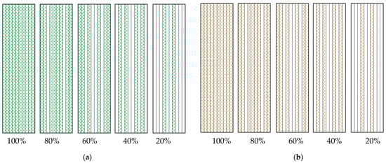
Figure 2.
Schematic of the vegetation cover designs for the simulated rainfall experiments. (a) Photosynthetic vegetation; (b) non-photosynthetic vegetation.
2.2.4. Calculation of Vegetation Cover
- (1)
- Calculation of photosynthetic vegetation cover
The photosynthetic vegetation cover was based on the Technical Guidelines for Dynamic Monitoring of Soil Erosion. The NDVI product MOD13Q1 was downloaded for the study year, as were 24 half-months of MODIS remote sensing data during the first 3 years of the study. The vegetation index NDVI was then converted to vegetation cover [46] using the following formula:
where refers to the minimum NDVI value and refers to the maximum NDVI value.
- (2)
- Calculation of non-photosynthetic vegetation cover
Drawing on the research findings from similar study areas, the DFI index was used as the non-photosynthetic vegetation index to calculate its vegetation cover [47]. According to the band characteristics of MODIS and Landsat 8 OLI images, the corresponding band of Landsat 8 OLI images was used to replace the response band in the DFI index to obtain a DFI index applicable to Landsat 8 OLI images using the formula shown in Equation (10) [48,49]. This DFI index was then used to calculate the non-photosynthetic vegetation cover (Equation (11)).
where , , , and denote the infrared band (red), the near-infrared band (NIR), the short-wave infrared-1 band (SWIR 1), and the short-wave infrared-2 band (SWIR 2), respectively, of Landsat 8 OLI images.
2.2.5. Statistical Analysis
To explore the differences between the four methods, this study quantified the differences between two methods by calculating the root mean square error. The root mean square error calculation formula is
In this study, is the result of a certain method at the ith point, and is the result of another method at the ith point.
Correlation analysis was used to verify the accuracy and rationality of the C/B factor values obtained using the four methods. Specifically, the judgment standard used in this study was the Pearson correlation coefficient.
2.3. Data Sources
Incorporating the content of this study, the data involved mainly included meteorological data, elevation data, land use data, soil data, NDVI data, and DFI data. The sources of these data are shown in Table 1.

Table 1.
Sources of data required for this study.
3. Results
3.1. Results of the C/B Factor
We conducted a statistical analysis of the four calculated C/B factors, which mainly included frequency histograms of the factor calculation results, their characteristic values, and the distribution over 24 half-months of the year.
As demonstrated in Figure 3 and Figure 4, the analysis of the annual average C/B factors revealed that the maximum value for the B factor was 1, while the minimum was 0. The data primarily clustered in three segments: 0, 0–0.05, and 1, with the segment containing the value 1 showing the largest proportion. Similarly, the maximum value for was also 1, with a minimum of 0, and the values were concentrated in three segments: 0, 0–0.9, and 1, although most values were found to be between 0 and 0.1. In contrast, and were continuously distributed. For , the maximum value was 0.9559, the minimum was 0.0127, and the distribution was concentrated in the range of 0.02–0.2. had a maximum value of 0.0489 and a minimum of 0.0134, with its values concentrated in the segment of 0.02–0.04. The mean values of the four C/B factors were ranked as follows: B > > > . When examining the annual average C/B factors specific to forest land, gardens, and grassland, all the factors except showed a continuous distribution. The B factor appeared to range from 0.0058 to 0.4906, primarily concentrated between 0.05 and 0.2. The values ranged from 0 to 1, following a distribution trend similar to that of the annual average factors. The value was distributed between 0.0159 and 0.7518, while spanned from 0.0138 to 0.4906. The distribution trends of the factors calculated using both the methods for forest land, gardens, and grassland generally aligned with the distribution trends of the annual average factors. The mean values for the C/B factors calculated for forest land, gardens, and grassland were ranked as follows: > > > B.
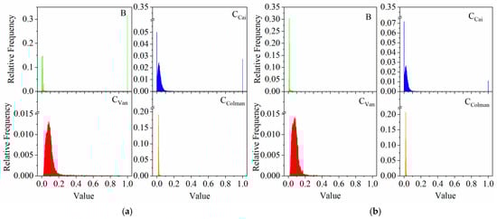
Figure 3.
Frequency distributions of the C/B factors in the study area. (a) All land use types; (b) specific categories: forest land, gardens, and grassland.
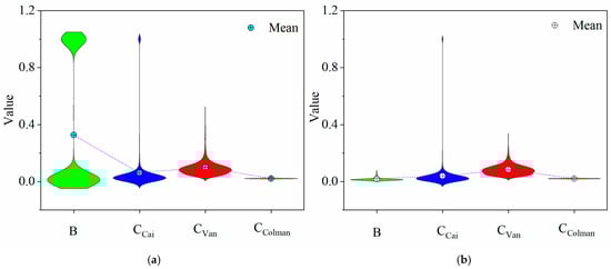
Figure 4.
Descriptive statistics of the C/B factors in the study area. (a) All land use types; (b) specific categories: forest land, gardens, and grassland.
According to the calculation rules, we obtained the C/B factors for each half-month for forest land, gardens, and grassland (Figure 5). The B factor of each half-month of the year was much larger than the factor calculated using the other three methods, while the of each half-month was smaller. The B and experienced relatively stable changes during the year. Among the four results, had the largest fluctuation during the year, and had the second largest fluctuation. At the same time, each result shows that the C/B factor was the smallest in the summer and the largest in the winter. For the C/B factor of forest land, gardens, and grassland, the trend of the factors calculated using the four methods was the same as that of the factors corresponding to all land use types, but the overall value was smaller than the factor of all land use types. It can be seen that the B and of forest land, gardens, and grassland were very close.
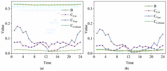
Figure 5.
Distribution of changes in C/B values over the 24 half-months of the year. (a) All land use types; (b) specific categories: forest land, gardens, and grassland.
To accurately identify the differences between the four methods, this study quantified the differences between the two methods through the root mean square error (Figure 6). The analysis results show that for the annual average vegetation coverage and management factor, the B value differed greatly from the other three results, with a root mean square error greater than 0.5. The largest difference was between the B and , which had an RMSE of 0.5637. The difference between and was the smallest, with an RMSE of 0.1125. For the C/B factors of forest land, gardens, and grassland, the RMSE values of the four methods were relatively small, with the largest being only 0.1072, which resulted from the comparison between and . Meanwhile, the difference between the B and was the smallest, with their RMSE value being only 0.0373.
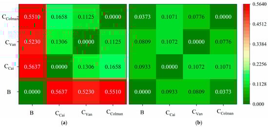
Figure 6.
Comparison of the root mean square error between the two methods. (a) All land use types; (b) specific categories: forest land, gardens, and grassland.
3.2. Applicability Analysis of the C/B Factors
To ensure the accuracy and reasonableness of the C/B factor values, this study collected the published research results in regions with similar natural environments to the study area. The results were cited more often (Clit), which indicates that the assignment of values was reasonable and has been recognized by a larger number of people. We counted the C/B factors of the four methods according to land use types. We correlated them with Clit (Table 2), which showed that Clit had the highest correlation with the B factor and the correlation parameter was meaningful (Pearson correlation = 0.853, p = 0.007).
Table 2.
Correlation analysis results of Clit and the C/B factors calculated using the four different calculation methods.
In addition, the area of soil erosion intensity corresponding to the four C/B factor methods was counted based on land use types (Figure 7). As can be seen from the results, for the areas with land use types of rivers, lakes, reservoirs, and ponds, the soil erosion intensity calculated using the four different C/B factor methods was classified as light erosion. However, the results corresponding to , , and showed some variation in erosion intensities. In reality, we generally consider that rivers, lakes, reservoirs, and ponds do not experience erosion. Based on the erosion class classification standard, the observed intensity is typically categorized as light erosion. For dry lands, the soil erosion intensities calculated using the three C/B methods (, , and ) were mainly focused on light erosion, with yielding only light erosion. The soil erosion results calculated using the B factor, on the contrary, showed that dry lands had different amounts of each soil erosion intensity, and the size of the area was as follows: moderate erosion > mild erosion > intensive erosion > light erosion > strong erosion > severe erosion. As the study area is fragmented and the dry lands are mostly sloping cultivated land, coupled with human cultivation, the erosion intensity of the dry lands was usually higher, and the soil erosion status calculated using the B factor was more in line with reality.
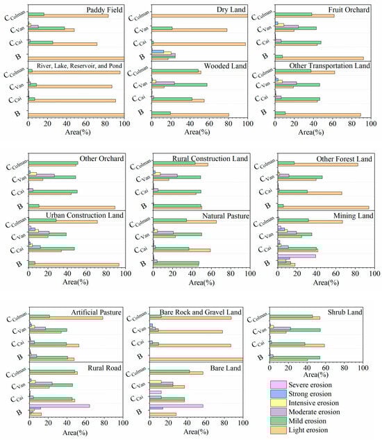
Figure 7.
Area of soil erosion corresponding to different land use types calculated using the four C/B factor calculation methods.
In conclusion, from the standpoint of statistical analysis and in terms of its proximity to reality, it is posited that the B factor is the most accurate and reasonable.
3.3. Establishment of the Relationship Equation for Integrated Vegetation Cover
According to the sand production process of photosynthetic and non-photosynthetic vegetation, as shown in Figure 8, the overall sand production rate for photosynthetic vegetation decreased with the increase in vegetation cover. However, there was not much difference in the sand production rate under each vegetation cover, especially since the sand production rates were very close at 80% and 100% vegetation cover, and the sand production rate of photosynthetic vegetation was less than 0.01 g/s under any vegetation cover. For non-photosynthetic vegetation, the sand production rate at 20% vegetation cover was much greater than that at the other higher vegetation cover, and the difference in sand production rate at the other higher vegetation cover was not significant. However, the overall sand production rate of non-photosynthetic vegetation was greater than the sand production rate of photosynthetic vegetation under the same cover.
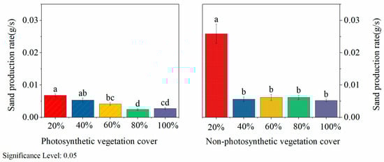
Figure 8.
Comparison of the sand production rate between photosynthetic vegetation and non-photosynthetic vegetation. Different small letters indicate significant differences between groups.
Figure 9 shows the total sand production for the whole rainfall. Under the same vegetation cover, the sand production of non-photosynthetic vegetation was greater than that of photosynthetic vegetation, and the change in sand production under both types of cover was more drastic when the vegetation cover was less than 40%.
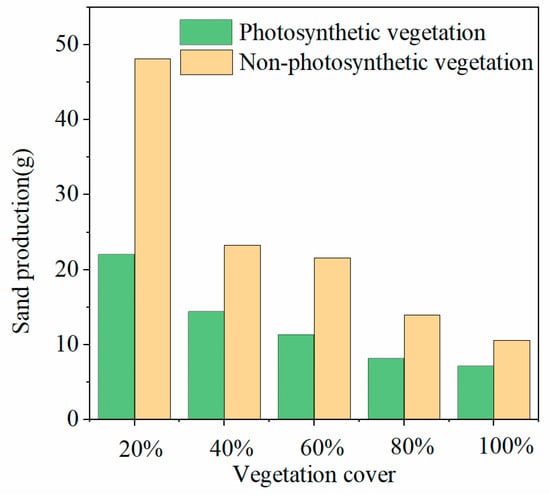
Figure 9.
Comparison of total sediment production between photosynthetic vegetation and non-photosynthetic vegetation.
Combined with the data on sand production without vegetation cover, this study first formulated a relationship equation between the degree of non-photosynthetic vegetation cover and the amount of sand production. Then, the amount of sand production under photosynthetic vegetation cover was introduced into the relationship equation to calculate the degree of non-photosynthetic vegetation cover under the same sand production conditions to fit the relationship between the degree of photosynthetic vegetation cover and the degree of non-photosynthetic vegetation cover. When calculating non-photosynthetic vegetation cover, it is possible to determine the photosynthetic vegetation cover that provides the same benefits for soil and water conservation. This allows for the calculation of the integrated vegetation cover. The results are presented in Figure 10, and the formula for calculating the integrated vegetation cover is provided in Equation (13).
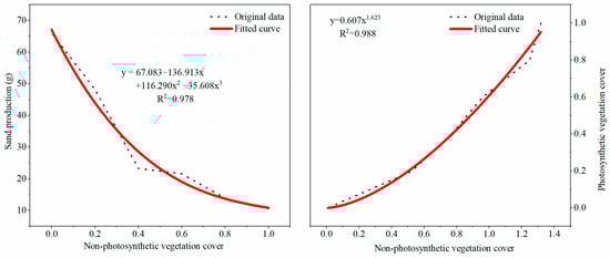
Figure 10.
Fitting the relationship between photosynthetic vegetation and non-photosynthetic vegetation.
3.4. Correction of the C/B Factor Calculation Methods
Considering the seasonal variation of non-photosynthetic vegetation cover and the Landsat 8 OLI imaging period and quality, in this study, one phase of imagery in 2022 with less than 10% cloud cover was selected as the data source for the DFI index calculation in January–March, April–June, July–September, and October–December. Based on the DFI index formula (Equation (9)) and the non-photosynthetic vegetation cover formula (Equation (10)), the non-photosynthetic vegetation cover was obtained (Figure 11). It can be seen from the graph that overall, the Lizixi watershed had the greatest non-photosynthetic vegetation cover from October to December and the least non-photosynthetic vegetation cover from July to September, while the difference between the months of January–March and April–June was not significant. From a spatial point of view, the larger non-photosynthetic vegetation cover was mainly concentrated in the middle of the watershed and at the watershed boundary. By counting the characteristic values of non-photosynthetic vegetation cover (Table 3), it can be seen that the mean value of non-photosynthetic vegetation cover in January–March was larger than that in April–June.
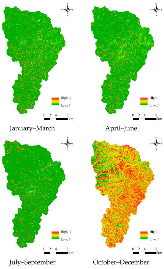
Figure 11.
Coverage of non-photosynthetic vegetation in the fourth period of 2023.
Table 3.
Statistical characteristic values of non-photosynthetic vegetation coverage.
The 24 half-month photosynthetic vegetation cover in 2023 is shown in Figure 12, which shows that the photosynthetic vegetation cover shifted with the seasons. The highest vegetation cover occurred in the summer and the lowest in the winter, and the high vegetation cover was mainly distributed in the northern and southern parts of the watershed.
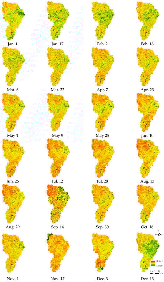
Figure 12.
Photosynthetic vegetation coverage in the 24 half-months of 2023.
The converted January–March non-photosynthetic vegetation cover was added to the photosynthetic vegetation cover for the first six half-month periods, and this process continued for all 24 periods to obtain the integrated vegetation cover, which was then used to correct the B factor. At the same time, the photosynthetic vegetation cover data without adding the non-photosynthetic vegetation cover were brought into the formula to calculate the B factor before correction, and the corrected B factor was then subtracted from the B factor before correction. The results show that the maximum difference between the two was 0, indicating that the corrected B factor was smaller than the one before correction, and the correction results are reliable.
4. Discussion
4.1. The Applicability of the C/B Factor Calculation Methods in the Purple Soil Hilly Region
The initial outcome of this study was the identification of the most suitable method for calculating the C/B factor in the purple soil hilly region from the four most widely used methods currently in use, including the B factor calculation method. A detailed analysis was conducted on the origins and calculation formulas of the four methods. The calculation method is a linear relationship established based on NOAA AVHRR image data for assessing soil erosion in continental Europe and, in a later study [50,51,52,53,54], it was pointed out that the setting of α and β also needs to be considered regarding the type of remote sensing imagery used. At the same time, the soil erosion environment in continental Europe is quite different from that in the purple soil hilly area of China and, so, the applicability is low from a macroscopic point of view. Similarly, the calculation method is modified from the relational equation established by V.L. Durigon [55] in the tropics with high rainfall intensities, with significant differences in parameter values and areas of applicability from the present study area. The calculation method, to the contrary, estimates the vegetation cover through the vegetation index, which further increases the uncertainty. However, the B factor calculation results are more in line with reality as this method considers land use types in the calculation, where some land use types are directly assigned values and seasonal changes are also considered.
From the frequency distributions and descriptive statistics of the four factors under all land use types, it is evident that the distribution characteristics of the calculation results of the four factors differ significantly. However, for forest land, gardens, and grassland, both the statistical features and the RMSE calculation results indicate that the differences between the B and the calculation results are the smallest. Nevertheless, the parameters required for the calculation of the B calculation method are relatively complex. When the relevant parameters are unavailable, the calculation method can serve as an alternative.
However, the four methods are empirical equations which themselves have certain limitations. It has been pointed out that the NDVI only reflects information on the green part of the surface vegetation and is unable to detect the protective effect of surface dead leaves and other mulch covering the soil, which is very likely to cause an overestimation of the C/B factor of forested land [56]. In addition, the NDVI data have the problems of background pollution, saturation, and non-linearity, and the empirical regression model relies on a large amount of measured data, so it is only suitable for specific regions and not universal [57]. Therefore, selecting an applicable C/B factor calculation method for a specific area is the key to assessing soil erosion. In this study, the most appropriate C/B factor calculation method for the purple soil hilly region was identified as the B factor after comparing Clit.
4.2. Correction of the C/B Factor Calculation Method for the Purple Soil Hilly Region
The B calculation method is widely recognized both in the research field and in practical applications [58]. However, the calculation method only considers the effect of photosynthetic vegetation on soil erosion, ignoring the role of non-photosynthetic vegetation. In this study, the modified B factor method retained the rich accumulation of the original B factor calculation method. Additionally, it reflected the effect of non-photosynthetic vegetation on erosion and sand production in the factorization in a simpler way. The Three Gorges Reservoir Soil and Water Conservation and Environment Research Station is located on the left bank of the middle reaches of the Three Gorges Reservoir in Shibao, Zhong County, Chongqing Municipality, with the geographic coordinates of 108°10′ E, 30°25′ N, which is 30 km from the city center of Zhong County. The research station and the Lizixi watershed both have purple soils, and the climate type is the same as that of the central subtropical temperate monsoon climate. Additionally, the topography, landforms, and vegetation types are all of a high degree of similarity [59,60]. Therefore, the experimental results obtained using the Three Gorges Reservoir Area Soil and Water Conservation and Environment Research Station as a platform could be applied to the Lizixi watershed.
The results of the non-photosynthetic vegetation cover calculation showed a clear seasonal effect, with high non-photosynthetic vegetation cover in the winter and low cover in the summer. The photosynthetic vegetation cover showed the opposite phenomenon, with the highest photosynthetic vegetation cover occurring in the summer and the lowest in the winter. The Lizixi watershed belongs to the central subtropical temperate monsoon climate, which is characterized by warm springs, cool autumns, hot summers, and cold winters, with four distinct seasons. The present study has demonstrated that vegetation growth is subject to climatic change, with the photosynthetic vegetation flourishing in the summer and the non-photosynthetic vegetation in the winter. This finding is consistent with the characteristics of the photosynthetic and non-photosynthetic vegetation cover calculated in the present study, thereby indicating the credibility of the results of the calculations. The high photosynthetic vegetation cover is mainly distributed in the north and south of the watershed because the land use type in this part of the basin is mainly woodland and the tree cover is high [61,62,63]. Before correcting the B factor, only the protective effect of photosynthetic vegetation on the soil was considered. However, non-photosynthetic vegetation can also provide a protective layer for the soil to reduce soil erosion. Hence, the value of the B factor before correction was greater than the corrected B factor, which took into account the protective effect of non-photosynthetic vegetation on the soil. This result is a reflection of the role of non-photosynthetic vegetation in soil and water conservation.
5. Conclusions
Our results demonstrate that the B calculation method is the most appropriate for calculating soil erosion in the purple soil hilly region. The B calculation method exhibited the highest correlation with the literature values () and produced soil erosion estimates that were closer to reality when compared with other methods. This finding underscores the importance of selecting region-specific C/B factor calculation methods to enhance the accuracy of soil erosion assessments.
Furthermore, our study highlights the significant role of non-photosynthetic vegetation in soil and water conservation. The results from the artificial rainfall experiments revealed the relationship between photosynthetic vegetation cover, non-photosynthetic vegetation cover, and soil erosion. By incorporating non-photosynthetic vegetation cover into the B factor calculation, we derived a corrected B factor that was smaller than the pre-correction value. This correction effectively accounted for the protective effect of non-photosynthetic vegetation, thereby improving the reliability of soil erosion predictions.
This study established a cost-effective framework for optimizing C/B factor estimation in USLE series model applications across purple soil hilly regions, resolving the dual challenges relating to the economic constraints of traditional methods and the regional adaptability limitations of remote sensing approaches. Future research should focus on further validating the proposed methods in different environmental settings in order to ensure their generalizability. Additionally, exploring the integration of more advanced remote sensing technologies and machine learning algorithms could enhance the accuracy and efficiency of C/B factor calculations.
Author Contributions
Conceptualization, R.C. and Y.Z.; methodology, R.C. and A.W.; software, R.C.; validation, D.W., W.W., and B.B.; formal analysis, R.C.; investigation, Y.L.; resources, J.F.; writing—original draft preparation, R.C.; writing—review and editing, R.C.; visualization, T.J.; supervision, J.Z. All authors have read and agreed to the published version of the manuscript.
Funding
This research was funded by the Power Construction of China (grant number P60224) and the National Key R&D Program of China (2016YFC0402301-02).
Institutional Review Board Statement
Not applicable.
Data Availability Statement
The data presented in this study are available upon request from the corresponding author. The data are not publicly available due to privacy.
Acknowledgments
The authors would like to express their sincere gratitude to the editors and reviewers who put considerable time and effort into their comments on this paper.
Conflicts of Interest
The authors declare no conflicts of interest.
References
- Bai, L.; Wang, N.; Jiao, J.; Chen, Y.; Tang, B.; Wang, H.; Chen, Y.; Yan, X.; Wang, Z. Soil erosion and sediment interception by check dams in a watershed for an extreme rainstorm on the Loess Plateau, China. Int. J. Sediment Res. 2020, 35, 408–416. [Google Scholar] [CrossRef]
- Lizaga, I.; Latorre, B.; Gaspar, L.; Navas, A. Consensus ranking as a method to identify non-conservative and dissenting tracers in fingerprinting studies. Sci. Total Environ. 2020, 720, 137537. [Google Scholar] [CrossRef]
- Wang, X.; Zhao, X.; Zhang, Z.; Yi, L.; Zuo, L.; Wen, Q.; Liu, F.; Xu, J.; Hu, S.; Liu, B. Assessment of soil erosion change and its relationships with land use/cover change in China from the end of the 1980s to 2010. Catena 2016, 137, 256–268. [Google Scholar] [CrossRef]
- Batista, P.V.G.; Davies, J.; Silva, M.L.N.; Quinton, J.N. On the evaluation of soil erosion models: Are we doing enough? Earth-Sci. Rev. 2019, 197, 102898. [Google Scholar] [CrossRef]
- Boyle, J.F.; Plater, A.J.; Mayers, C.; Turner, S.D.; Stroud, R.W.; Weber, J.E. Land use, soil erosion, and sediment yield at Pinto Lake, California: Comparison of a simplified USLE model with the lake sediment record. J. Paleolimnol. 2011, 45, 199–212. [Google Scholar] [CrossRef]
- Mondal, A.; Khare, D.; Kundu, S. A comparative study of soil erosion modelling by MMF, USLE and RUSLE. Geocarto Int. 2016, 33, 89–103. [Google Scholar] [CrossRef]
- Demirci, A.; Karaburun, A. Estimation of soil erosion using RUSLE in a GIS framework: A case study in the Buyukcekmece Lake watershed, northwest Turkey. Environ. Earth Sci. 2011, 66, 903–913. [Google Scholar] [CrossRef]
- Mallick, J.; Alashker, Y.; Mohammad, S.A.-D.; Ahmed, M.; Hasan, M.A. Risk assessment of soil erosion in semi-arid mountainous watershed in Saudi Arabia by RUSLE model coupled with remote sensing and GIS. Geocarto Int. 2014, 29, 915–940. [Google Scholar] [CrossRef]
- Das, B.; Bordoloi, R.; Thungon, L.T.; Paul, A.; Pandey, P.K.; Mishra, M.; Tripathi, O.P. An integrated approach of GIS, RUSLE and AHP to model soil erosion in West Kameng watershed, Arunachal Pradesh. J. Earth Syst. Sci. 2020, 129, 94. [Google Scholar] [CrossRef]
- Renard, K.; Foster, G.; Weesies, G.; McCool, D.; Yoder, D. RUSLE a guide to conservation planning with the revised universal soil loss equation. In USDA Agriculture Handbook; United States Department of Agriculture: Washington, DC, USA, 1997; Volume 703. [Google Scholar]
- Liu, B.; Zhang, K.; Yun, X. An Empirical Soil Loss Equation. In Proceedings of the 12th ISCO Conference, Beijing, China, 26–31 May 2002. [Google Scholar]
- Liu, B.; Xie, Y.; Zhang, K. Soil Erosion Prediction Model; China Science and Technology Press: Beijing, China, 2001. [Google Scholar]
- Zang, J.; Zuo, C.; Li, X. Probe of the Effect of Natural Factors on Soil Erosion. J. Anhui Agric. Sci. 2008, 3, 1140–1141+1176. [Google Scholar] [CrossRef]
- Wen, X.; Deng, X.; Zhang, F. Scale effects of vegetation restoration on soil and water conservation in a semi-arid region in China: Resources conservation and sustainable management. Resour. Conserv. Recycl. 2019, 151, 104474. [Google Scholar] [CrossRef]
- Almagro, A.; Thomé, T.C.; Colman, C.B.; Pereira, R.B.; Marcato Junior, J.; Rodrigues, D.B.B.; Oliveira, P.T.S. Improving cover and management factor (C-factor) estimation using remote sensing approaches for tropical regions. Int. Soil Water Conserv. Res. 2019, 7, 325–334. [Google Scholar] [CrossRef]
- Wischmeier, W.H.; Smith, D.D. Predicting Rainfall Erosion Losses—A Guide to Conservation Planning; United States Department of Agriculture: Washington, DC, USA, 1978. [Google Scholar]
- Wanzhong, W.; Juying, J. Qutantitative evaluation on factors influencing soil erosion in China. Bull. Soil Water Conserv. 1996, 5, 1–20. [Google Scholar]
- Yan, Z.; Baoyuan, L.; Peijun, S.; Zhongshan, J. Crop cover factor estimating for soil loss prediction. Acta Ecol. Sin. 2001, 21, 1050–1056. [Google Scholar]
- Hongxia, X. Evaluation of Spatial and Temporal Changes of Soil Erosion and Environmental Effect of Soil and Water Conservation in Yanhe River Basin. Ph.D. Thesis, Shaanxi Normal University, Xi’an, China, 2008. [Google Scholar]
- Fan, J.; Wang, N.; Chen, G.; Jiao, J.; Xie, Y. Practice factor of soil and water conservation in Northeastern China. Sci. Soil Water Conserv. 2011, 9, 75–78+92. (In Chinese) [Google Scholar]
- Guo, J.; Gu, Z.; Yuan, S.; Zhang, K. Calculation and Evaluation of Factor Values of Soil and Water Conservation Measures in Southwest Karst Area. Soil Water Conserv. 2014, 10, 50–53+71. (In Chinese) [Google Scholar]
- Xin, Y.; Liu, G.; Xie, Y.; Gao, Y.; Liu, B.; Shen, B. Effects of soil conservation practices on soil losses from slope farmland in northeastern China using runoff plot data. Catena 2019, 174, 417–424. [Google Scholar] [CrossRef]
- Chen, H.; Zhang, X.; Abla, M.; Lü, D.; Yan, R.; Ren, Q.; Ren, Z.; Yang, Y.; Zhao, W.; Lin, P.; et al. Effects of vegetation and rainfall types on surface runoff and soil erosion on steep slopes on the Loess Plateau, China. Catena 2018, 170, 141–149. [Google Scholar] [CrossRef]
- Yu, S.; Eerdun, H.; Huishi, D. Application of Vegetation Cover in Soil Erosion Modulus Calculation. Bull. Soil Water Conserv. 2013, 33, 185–189+309. [Google Scholar]
- Shi, T.; Jianxiang, L.; Ke, Z.; Zhiqiang, W. Research on Potential Soil Erosion in the He-Long Region of the Middle Reaches of the Yellow River. J. Nat. Sci. Hunan Norm. Univ. 2014, 37, 1–6. [Google Scholar]
- Chongfa, C.; Shuwen, D.; Zhihua, S.; Li, H.; Guanyuan, Z. Study of Applying USLE and Geographical Information System IDRISI to Predict Soil Erosion in Small Watershed. J. Soil Water Conserv. 2000, 14, 19–24. [Google Scholar]
- Knijff, J.; Jones, R.; Montanarella, L. Soil Erosion Risk Assessment in Italy; European Soil Bureau: Brussels, Belgium, 2002. [Google Scholar]
- Barbosa Colman, C.; Oliveira, P.T.; Almagro, A.; Filho, B. Impacts of Climate and Land Use Change on Soil Erosion in the Upper Paraguay Basin. In Proceedings of the GRSS YP & ISPRS SC Summer School 2018, Campo Grande, Brazil, 29 October–1 November 2018. [Google Scholar]
- Guangzhen, W.; Jingpu, W.; Xueyong, Z.; Liu, H.; Min, Z. A Review on Estimating Fractional Cover of Non-photosynthetic Vegetation by Using Remote Sensing. Remote Sens. Technol. Appl. 2018, 33, 1–9. [Google Scholar]
- Guerschman, J.P.; Hill, M.J.; Renzullo, L.J.; Barrett, D.J.; Marks, A.S.; Botha, E.J. Estimating fractional cover of photosynthetic vegetation, non-photosynthetic vegetation and bare soil in the Australian tropical savanna region upscaling the EO-1 Hyperion and MODIS sensors. Remote Sens. Environ. 2009, 113, 928–945. [Google Scholar] [CrossRef]
- Tucker, C.J. Red and photographic infrared linear combinations for monitoring vegetation. Remote Sens. Environ. 1979, 8, 127–150. [Google Scholar] [CrossRef]
- Jingzhong, L. Study on Remote Sensing Extraction of Structural Vegetation Factors for Regional Soil Erosion. Master’s Thesis, Northwest University, Kirkland, WA, USA, 2009. [Google Scholar]
- Ting, Z. Remote Sensing Modeling of Structural Vegetation Cover in Yanhe River Basin, Northern Shaanxi, China. Master’s Thesis, Northwest University, Kirkland, WA, USA, 2013. [Google Scholar]
- Ding, L.; Fu, S.; Liu, B.; Yu, B.; Zhang, G.; Zhao, H. Effects of Pinus tabulaeformis litter cover on the sediment transport capacity of overland flow. Soil Tillage Res. 2020, 204, 104685. [Google Scholar] [CrossRef]
- Miura, S.; Ugawa, S.; Yoshinaga, S.; Keizo Hirai, T.Y. Floor Cover Percentage Determines Splash Erosion in Chamaecyparis obtusa Forests. Soil Sci. Soc. Am. J. 2015, 79, 1782–1791. [Google Scholar] [CrossRef]
- Chen, R.; Zhu, Y.; Zhang, J.; Wen, A.; Hu, S.; Luo, J.; Li, P. Determination of Contributing Area Threshold and Downscaling of Topographic Factors for Small Watersheds in Hilly Areas of Purple Soil. Land 2024, 13, 1193. [Google Scholar] [CrossRef]
- Ruiyin, C.; Dongchun, Y.; Anbang, W.; Chenggang, L.; Zhonglin, S. Research on Soil Erosion in Key Prevention and Control Region of Soil and Water Loss Based on GIS/CSLE in Sichuan Province. J. Soil Water Conserv. 2020, 34, 17–26. [Google Scholar]
- Knijff, J.M.v.d.; Jones, R.J.A.; Montanarella, L. Soil Erosion Risk Assessment in Europe; European Soil Bureau: Brussels, Belgium, 2000. [Google Scholar]
- Suhua, F.; Baoyuan, L.; Guiyun, Z.; Zhongxuan, S.; Xiaoli, Z. Calculation tool of topographic factors. Science of Soil and Water Conservation 2015, 13, 105–110. [Google Scholar]
- Zhang, H.; Zhang, R.; Qi, F.; Liu, X.; Niu, Y.; Fan, Z.; Zhang, Q.; Li, J.; Yuan, L.; Song, Y.; et al. The CSLE model based soil erosion prediction: Comparisons of sampling density and extrapolation method at the county level. Catena 2018, 165, 465–472. [Google Scholar] [CrossRef]
- Huang, C.L.; Yang, Q.K.; Cao, X.Y.; Li, Y.R. Assessment of the Soil Erosion Response to Land Use and Slope in the Loess Plateau-A Case Study of Jiuyuangou. Water 2020, 12, 529. [Google Scholar] [CrossRef]
- Duan, X.; Bai, Z.; Rong, L.; Li, Y.; Ding, J.; Tao, Y.; Li, J.; Li, J.; Wang, W. Investigation method for regional soil erosion based on the Chinese Soil Loss Equation and high-resolution spatial data: Case study on the mountainous Yunnan Province, China. Catena 2020, 184, 104237. [Google Scholar] [CrossRef]
- Shi, W.; Huang, M.; Barbour, S.L. Storm-based CSLE that incorporates the estimated runoff for soil loss prediction on the Chinese Loess Plateau. Soil Tillage Res. 2018, 180, 137–147. [Google Scholar] [CrossRef]
- Liu, B.; Guo, S.; Li, Z.; Xie, Y.; Zhang, K.; Liu, X. Sampling survey of water erosion in China. Soil Water Conserv. 2013, 10, 26–34. (In Chinese) [Google Scholar]
- Li, Z.; Fu, S.; Liu, B. sampling program of water erosion inventory in the first national water resource survey. Sci. Soil Water Conserv. 2012, 10, 77–81. (In Chinese) [Google Scholar]
- Wang, X.; Jia, K.; Liang, S.; Li, Q.; Wei, X.; Yao, Y.; Zhang, X.; Tu, Y. Estimating Fractional Vegetation Cover From Landsat-7 ETM+ Reflectance Data Based on a Coupled Radiative Transfer and Crop Growth Model. IEEE Trans. Geosci. Remote Sens. 2017, 55, 5539–5546. [Google Scholar] [CrossRef]
- Chao, Z. Remote sensing inversion and analysis of temporal and spatial variations in the cover of dead leaf layer. Master’s Thesis, Northwest University, Kirkland, WA, USA, 2019. [Google Scholar]
- Cao, X.; Chen, J.; Matsushita, B.; Imura, H. Developing a MODIS-based index to discriminate dead fuel from photosynthetic vegetation and soil background in the Asian steppe area. Int. J. Remote Sens. 2010, 31, 1589–1604. [Google Scholar] [CrossRef]
- Daughtry, C.; Huntjr, E. Mitigating the effects of soil and residue water contents on remotely sensed estimates of crop residue cover. Remote Sens. Environ. 2008, 112, 1647–1657. [Google Scholar] [CrossRef]
- Santarsiero, V.; Lanorte, A.; Nolè, G.; Cillis, G.; Tucci, B.; Murgante, B. Analysis of the Effect of Soil Erosion in Abandoned Agricultural Areas: The Case of NE Area of Basilicata Region (Southern Italy). Land 2023, 12, 645. [Google Scholar] [CrossRef]
- Cao, Y.; Hua, L.; Tang, Q.; Liu, L.; Cai, C. Evaluation of monthly-scale soil erosion spatio-temporal dynamics and identification of their driving factors in Northeast China. Ecol. Indic. 2023, 150, 110187. [Google Scholar] [CrossRef]
- Achu, A.L.; Thomas, J. Soil erosion and sediment yield modeling in a tropical mountain watershed of the southern Western Ghats, India using RUSLE and Geospatial tools. Total Environ. Res. Themes 2023, 8, 100072. [Google Scholar] [CrossRef]
- Gitelson, A.A.; Kaufman, Y.J.; Merzlyak, M.N. Use of a green channel in remote sensing of global vegetation from EOS-MODIS. Remote Sens. Environ. 1996, 58, 289–298. [Google Scholar] [CrossRef]
- Van Leeuwen, W.J.; Sammons, G. Vegetation dynamics and soil erosion modeling using remotely sensed data (MODIS) and GIS. In Proceedings of the Tenth Biennial USDA Forest Service Remote Sensing Applications Conference, Salt Lake City, UT, USA, 5–9 April 2004; pp. 5–9. [Google Scholar]
- Durigon, V.L.; Carvalho, D.F.; Antunes, M.A.H.; Oliveira, P.T.S.; Fernandes, M.M. NDVI time series for monitoring RUSLE cover management factor in a tropical watershed. Int. J. Remote Sens. 2014, 35, 441–453. [Google Scholar] [CrossRef]
- Lei, W.; Wen, Z. Research on soil erosion vegetation factor index based on community structure. J. Soil Water Conserv. 2008, 22, 68–72. [Google Scholar]
- Zhengxing, W.; Chuang, L.; Alfredo, H. From AVHRR-NDVI to MODIS-EVI: Advances in vegetation index research. Acta Ecol. Sin. 2003, 23, 979–987. [Google Scholar]
- Liu, B.; Xie, Y.; Li, Z.; Liang, Y.; Zhang, W.; Fu, S.; Yin, S.; Wei, X.; Zhang, K.; Wang, Z.; et al. The assessment of soil loss by water erosion in China. Int. Soil Water Conserv. Res. 2020, 8, 430–439. [Google Scholar] [CrossRef]
- Yun, Z.; Lin, W. Runoff and Sediment Simulation in Purple Hilly Area Based on SWAT Model. Geo-Inf. Sci. 2013, 15, 401–407. [Google Scholar]
- Hua, D.; Ming, G.; Jiaxin, L.; Yingyan, W.; Zifang, W. Effects of Biochar and Straw Return on Soil Aggregate and Organic Carbon on Purple Soil Dry Slope Land. Environ. Sci. 2021, 42, 5481–5490. [Google Scholar] [CrossRef]
- Xiaoli, J.; Genwei, C.; Zelong, M.; Jihui, F. Modeling of Soil Erosion for Lizixi Basin in Sichuan Hilly Region. J. Sichuan Agric. Univ. 2012, 30, 56–59. [Google Scholar]
- Zhang, S.; Hou, X.; Wu, C.; Zhang, C. Impacts of climate and planting structure changes on watershed runoff and nitrogen and phosphorus loss. Sci Total Environ. 2020, 706, 134489. [Google Scholar] [CrossRef]
- Zhang, S.; Liu, Y.; Wang, T. How land use change contributes to reducing soil erosion in the Jialing River Basin, China. Agric. Water Manag. 2014, 133, 65–73. [Google Scholar] [CrossRef]
Disclaimer/Publisher’s Note: The statements, opinions and data contained in all publications are solely those of the individual author(s) and contributor(s) and not of MDPI and/or the editor(s). MDPI and/or the editor(s) disclaim responsibility for any injury to people or property resulting from any ideas, methods, instructions or products referred to in the content. |
© 2025 by the authors. Licensee MDPI, Basel, Switzerland. This article is an open access article distributed under the terms and conditions of the Creative Commons Attribution (CC BY) license (https://creativecommons.org/licenses/by/4.0/).