TSO-HA*-Net: A Hybrid Global Path Planner for the Inspection Vehicles Used in Caged Poultry Houses

Abstract

Traditional track-based inspection schemes for caged poultry houses face issues with vulnerable tracks and cumbersome maintenance, while existing rail-less alternatives lack robust, reliable path planners. This study proposes TSO-HA*-Net, a hybrid global path planner that combines TSO-HA* with topological planning, which allows the inspection vehicle to continuously traverse a predetermined trackless route within each poultry house and conduct house-to-house inspections. Initially, the spatiotemporally optimized Hybrid A* (TSO-HA*) is employed as the lower-level planner to efficiently construct a semi-structured topological network by integrating predefined inspection rules into the global grid map of the poultry houses. Subsequently, the Dijkstra’s algorithm is adopted to plan a smooth inspection route that aligns with the starting and ending poses, conforming to the network. TSO-HA* retains the smoothness of HA* paths while reducing both time and computational overhead, thereby enhancing speed and efficiency in network generation. Experimental results show that compared to LDP-MAP and A*-dis, utilizing the distance reference tree (DRT) for h₂ calculation, the total planning time of the TSO-HA* algorithm is reduced by 66.6% and 96.4%, respectively, and the stored nodes are reduced by 99.7% and 97.4%, respectively. The application of the collision template in TSO-HA* results in a minimum reduction of 4.0% in front-end planning time, and the prior collision detection further decreases planning time by an average of 19.1%. The TSO-HA*-Net algorithm achieves global topological planning in a mere 546.6 ms, thereby addressing the critical deficiency of a viable global planner for inspection vehicles in poultry houses. This study provides valuable case studies and algorithmic insights for similar inspection task.

1. Introduction

The sustained growth of poultry farming is catalyzing progress in both animal welfare and technological innovation [1]. The integration of smart equipment is becoming more prevalent across different components of unmanned poultry farming systems [2,3]. Cage-based rearing systems predominate in intensive poultry husbandry [4,5], characterized by centralized management that facilitates environmental adjustment, daily inspection, and poultry processing [6]. Regular inspections are essential for ensuring poultry health and welfare. However, the vertical and dense structure of coops presents substantial challenges for manual inspections. Inspectors are required to frequently ascend and descend lifting platforms, a process that is not only time-consuming, but also physically demanding. Moreover, inspectors are exposed to airborne particles and irritant gases, posing significant health risks. Consequently, there is an urgent need for automated inspection vehicles in cage-rearing systems to supplant the labor-intensive and physically taxing nature of manual inspections [7].

Inspection vehicles, integral to unmanned poultry farming systems, are used for autonomous patrolling and poultry behavior monitoring [8]. Path planning is crucial for the operation of inspection vehicles. Common types of inspection vehicles in poultry houses include orbital robots, automated guided vehicles (AGVs), and autonomous mobile robots (AMRs). The first two types of inspection device rely on physical guide lines for path planning, while AMRs utilize algorithmic path planners.

Orbital robots, which traverse fixed tracks on surfaces such as flooring, cages [9], and ceilings, are used for fixed-area inspections. The ChickenBoy, developed by Faromatics [10], is an example of such a system. However, most inspection vehicles are designed with wheeled chassis, using lightweight magnetic strips or colored tapes for navigation (AGVs). Feng et al. [11] combined RFID and magnetic tags to construct linear paths and aid vehicle turns. Li et al. [12] developed a coop inspection method using electromagnetic tracing and metal marks. Track-based systems face challenges such as tire wear and manure contamination, leading to track misalignment and detachment, which cause navigation and positioning errors. Additionally, track installation and maintenance are troublesome, requiring structural adjustments to accommodate changes in the operating environment and reliance on other physical media for cage positioning and checkpoint design. Due to their inability to autonomously plan paths, the functionality of such inspection vehicles is restricted.

The supremacy of rail-less inspection schemes stems from advances in mobile robot technology [13]. By leveraging breakthroughs in perception [14,15], planning, localization [16,17,18], and motion control, various functional modules can be integrated into AMRs to address complex and diverse inspection requirements. In terms of path planning in caged poultry houses, Peng [19] utilized the A* algorithm, known for its lowest time complexity, for single- and multi-point navigation in long corridors. Li [20] applied Dijkstra and A* algorithms for global path planning in straight corridors between cages based on ROS. Zhang [21] combined the A* algorithm with insertion and jump points, further enhancing the path planning with a Reeds-Shepp curve-based TEB algorithm on a differential-drive inspection vehicle. Han [22] employed 3D laser technology to extract the centerline of the passage in the poultry house to generate a path. However, the paths generated by these approaches were often twisted or intermittent, failing to fully meet the systematic inspection requirements nor optimally align with the caged poultry house environment. As a result, existing rail-less inspection schemes have yet to find a stable and reliable path planner.

The planning of inspection routes in caged poultry houses necessitates a balance between point-to-point and full-coverage path planning. The inspection vehicle must follow a fixed path and traverse corridors while also reaching “target points” (determined by higher-level decisions) via the shortest path. However, existing rail-less solutions typically assess only limited path segments and do not fully consider the environmental features of poultry settings, thus failing to comprehensively address the planning requirements [23]. Furthermore, current inspection vehicles follow a “one house, one vehicle” model, which limits house-to-house inspection and results in high vehicle costs for large-scale poultry farms.

To address these challenges, this study proposes TSO-HA*-Net, a novel global path planner for coop inspection. TSO-HA*-Net is a hybrid algorithm based on a pre-existing grid map of the poultry houses. Initially, a spatiotemporally optimized Hybrid A* (TSO-HA*) algorithm is employed as the underlying planning mechanism, incorporating inspection rules to rapidly construct a semi-structured topological network that reflects the actual inspection environment. Subsequently, connection points and a graph-based algorithm (Dijkstra) are applied to find the shortest path within the network, deriving a smooth path that aligns with the starting and ending poses while adhering to network constraints, thus delineating the inspection route. The objective of this study is to develop a feasible global planner capable of flexibly, continuously, and rapidly generating inspection routes that adhere to the constraints of a predefined topological network, highlighting the planner’s overall continuity and coherence. This enables the inspection vehicle to follow a fixed route and traverse corridors while reaching target locations via the shortest path. The planner is specifically designed to be adaptable to the unique environment of poultry houses, thereby fulfilling the stringent requirements for inspection routes within these facilities. Additionally, the planner is expected to be a foundation tool for achieving cross-regional and multi-vehicle inspections.

The main contributions of this study are as follows:

(1)

An improved Hybrid A* algorithm is proposed which demonstrates shorter computational time, reduced resource consumption, and a higher success rate when applied to high-resolution maps. This improvement is achieved through a new heuristic value calculation using the distance reference tree and simplified occupancy grid templates for collision detection.

(2)

A hybrid path planner called TSO-HA*-Net is proposed, integrating the improved HA* algorithm, specific inspection rules, and topological planning. This planner is efficient and flexible for planning inspection routes in large-scale maps, establishing an intermediate planning scheme between point-to-point and full-coverage path planning. It addresses the route requirements for coop inspection and adapts to the actual poultry house environment.

(3)

The rail-less navigation system based on the presented planning scheme offers a viable alternative to traditional electromagnetic and line-following navigation. This study provides valuable case studies and algorithmic references for inspection tasks in caged poultry houses and similar facilities.

2. Materials and Methods

2.1. Experimental Platform

Figure 1 shows the experimental inspection vehicle utilized in this study. It is an autonomous mobile robot equipped with decision-making capabilities and relies on sensors and algorithms for path planning and environmental perception. A functional diagram of the inspection vehicle is presented in Figure 2 to systematically introduce its architecture and operational framework, consisting of three main systems: perception, decision and planning, and control. This study focuses on an in-depth algorithmic investigation of the global planning component within the decision and planning system, specifically addressing the global path planning problem for the autonomous inspection vehicle.

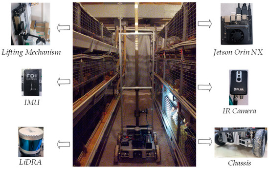
Figure 1. Experimental inspection vehicle.

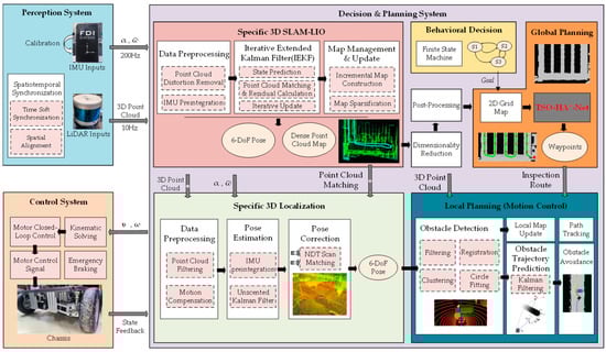
Figure 2. Functional diagram of the inspection vehicle.

2.2. Environmental Analysis and Mapping

The map serves as the foundation for global path planning in large-scale caged poultry farms. As shown in Figure 3, the site structure of such farms is characterized by poultry houses arranged in parallel rows, separated by passages. The interiors of houses contain multiple rows of stacked cages, which are interspersed with corridors. After map exploration [24], fusion [25,26], dimensionality reduction [27], and post-processing (e.g., artificially setting fixed obstacles), the environment of the poultry farm is accurately represented as a global occupancy grid map, providing a robust basis for the development and implementation of efficient path planning strategies. This study assumes that the map has been generated using the method above, and the target points are manually specified to simulate higher-level decision-making behavior.

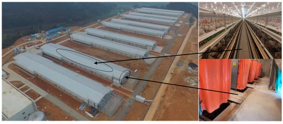
Figure 3. The site structure of a large-scale caged poultry farm.

The topological map [28] provides a concise graphical representation of the key nodes ${\varphi }_i$ and their interconnectedness (edges, $\overline{l}$) within the environment. When each edge is assigned the explicit orientation (i.e., $\overrightarrow{l}$) and a distance weight $l$, along with the rule constraint ${\mathrm{\Omega }}_i$ from $\overrightarrow{l_1}$ to $\overrightarrow{l_2}$, this type of topological map is referred to as a “semi-structured” topological network.

The TSO-HA*-Net algorithm is developed based on the fusion map shown in Figure 4, which integrates the grid map with the topological network. By artificially adding ${\varphi }_i$ into the grid map, the semi-structured topological network is obtained using the TSO-HA* algorithm as detailed in Section 2.5, where $\overrightarrow{l}$ and $\mathrm{\Omega }$ are defined by inspection requirements.

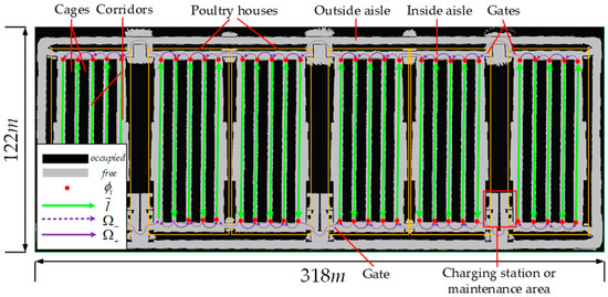
Figure 4. Fusion map of the caged poultry houses.

2.3. Problem Description

Efficient path planning plays a crucial role in optimizing operational time and avoiding inefficient navigation strategies. To ensure collision-free movement and enable the onboard camera to maintain an expansive forward field of view for identifying unhealthy chickens, the inspection vehicle should adhere to a straight trajectory as much as possible while traversing corridors. Considering the multiple “U”-shaped bends, it is essential to design smooth, appropriately curved paths along these turns to minimize motor strain and reduce tire wear. Moreover, seamless interconnectivity between topological edges is crucial for the smooth entry and exit of the inspection vehicle.

In this study, the Hybrid A* (HA*) algorithm is introduced, which incorporates motion constraints and accounts for initial and final poses [29,30]. However, the traditional HA* algorithm faces challenges such as slow planning speed, high resource consumption, and low success rate when applied to single, large-scale, and high-resolution maps [31,32,33]. To address these issues, an improved algorithm called TSO-HA* is proposed, with a new heuristic value calculation based on a K-dimensional tree and the KNN algorithm, along with rapid collision detection using simplified occupancy grid templates, which optimizes HA* in both temporal and spatial dimensions. TSO-HA* enables the rapid and efficient planning of collision-free, smooth paths with curvature constraints directly on the original-resolution grid map, thereby providing a robust algorithmic foundation for successful topological planning in a single operation.

Furthermore, the inspection vehicle typically follows a fixed route, and the route can be preplanned based on specific inspection requirements. This study further proposes a hybrid path planner, TSO-HA*-Net, that integrates the TSO-HA* algorithm, inspection rules, and topological planning, enabling the rapid generation of a complete inspection route. Commonly used graph-based path planning approaches include Dijkstra, A*, Floyd–Warshall, and Bellman–Ford algorithms. In the context of topological planning, the primary challenge is to compute the single-source shortest paths in sparse graphs. Dijkstra is a well-suited solution for this problem, leveraging a priority queue to ensure low computational overhead. However, A* performs suboptimally in the absence of accurate heuristic information, and designing an effective heuristic function remains a significant challenge. The Floyd–Warshall algorithm is suitable for computing shortest paths between all pairs of nodes, but it becomes redundant when only the path from a single source to a target is required. Moreover, its high computational complexity, $O_t(V^3)$ and $O_s(V^2)$, make it unsuitable for the spatiotemporal optimization scope discussed in this study. The Bellman–Ford algorithm, although more general and capable of handling graphs with negative-weight edges, also faces similar computational complexity issues.

A semi-structured topological network, combined with connection points, is introduced for topological planning, employing a specific Dijkstra’s algorithm and the Hash map to derive the shortest inspection route.

2.4. Overall Framework

The proposed planner consists of two parts: the lower-level TSO-HA* module and the upper-level topological planning module. Essentially, it performs the task of planning a topological network and determining a route within the network. The overall flowchart is shown in Figure 5. The main steps are as follows:

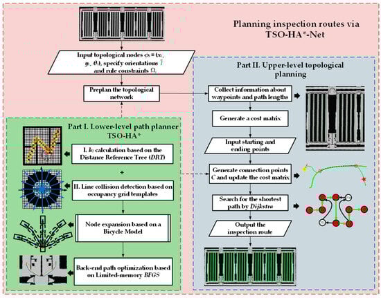
Figure 5. Flowchart for planning inspection routes via TSO-HA*-Net.

(1)

Adding pairs of starting and ending points with poses on the grid map as key topological nodes ${\varphi }_i$, and designating topological connections $\overrightarrow{l}$, ${\mathrm{\Omega }}_i$ on the basis of the required inspection rules.

(2)

Deploying the global planning algorithm TSO-HA* for path preplanning.

(3)

Saving all the information about path lengths and waypoints preplanned to form a semi-structured topological network of the poultry houses, which is then abstracted into a cost matrix guided by the path lengths.

(4)

Designating a new pair of starting and ending points in the network, with connection points generated, the network, and the corresponding matrix dynamically updated.

(5)

Using Dijkstra’s algorithm to search for an inspection route within the network, resulting in a complete inspection route for the poultry houses.

2.5. TSO-HA*: Lower-Level Path Planner

In contrast to the A* algorithm, which expands nodes based on grid-based four or eight neighborhoods [34], the HA* algorithm incorporates kinematics or dynamics constraints. By considering the node’s pose $\theta$ as an additional computational dimension, HA* allows for a more flexible expansion strategy, resulting in smoother paths that better conform to actual motion. The TSO-HA* algorithm inherits the advantages of HA* while enhancing computational efficiency in both time and space through a refined node expansion strategy, the distance reference tree and simplified occupancy grid templates. It is employed for path planning between topological nodes, resulting in the creation of a semi-structured topological network.

2.5.1. Node Expansion

Given an HA* node $S_k=\left(x_k,y_k,{\theta }_k\right)\in {ℝ}^2\times {\mathbb{Z}}^1$ at time $k$ in the grid map, the node expansion under low-speed conditions can be accomplished using a simplified bicycle model, as shown in Figure 6. In an extremely short time step $\Delta t$, the vehicle’s motion can be approximated as traveling in its current direction, with the arc length of the single-step movement $l_0$ equaling the vehicle’s travel distance. By employing the discrete bicycle kinematic model in Equations (1) and (2), the pose of the neighboring node $S_{k+1}=\left(x_{k+1},y_{k+1},{\theta }_{k+1}\right)$ at time $k+1$ can be derived, referred to as the motion primitive:

$$\left[\begin{array}{c}{x}_{k+1}\\ y_{k+1}\\ {\theta }_{k+1}\end{array}\right]=\left[\begin{array}{c}{x}_k\\ y_k\\ {\theta }_k\end{array}\right]+l_0\cdot \left[\begin{array}{c}cos{\theta }_k\\ sin{\theta }_k\\ tan{\phi }_i/L\end{array}\right]$$

(1)

$${\phi }_i=-{\phi }_{max}+{\displaystyle \frac{2{\phi }_{max}}{N-1}}\cdot i, i=0,1,\dots ,N-1$$

(2)

where the steering angle ${\phi }_i=f({\phi }_{max},N)$ is determined by the orientation subdivision number $N$ and the maximum steering angle ${\phi }_{max}$; $L$ represents the wheelbase.

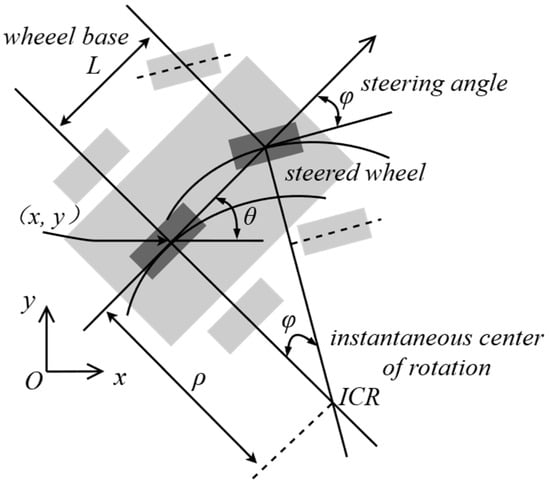
Figure 6. Bicycle kinematic model with the rear axle center as the origin.

In this study, a relatively smaller value of ${\phi }_{max}$ is chosen to plan paths with a larger curvature radius. The curvature radius $\rho =L/tan\phi$ determines the path curvature constrained by the steering angle $\phi$. Detailed parameters are shown in Table 1.

Table 1. Parameters for node expansion.

Parameters	Description	Value
${\delta }_{xy}$	Spatial resolution of the grid map	0.1 m
${\delta }_{\theta }$	Angular resolution of the grid map	5°
${\phi }_{max}$	Maximum steering angle	20°
$N$	Number of the orientation subdivision	5
$n$	Times of node expansion in each orientation	3
$l_0$	Arc length for a single-step movement	0.5 m
$L$	Wheelbase	0.48 m
$l_0^{\prime }$	Length of each segment of the DB curve	0.5 m
${\gamma }_1$	Curvature radius of the DB curve for TSO-HA* planning	2.3 m
${\gamma }_2$	Curvature radius of the DB curve for topological planning	0.3 m

As shown in Figure 7, the expansion of nodes starting from the current node $S=(x,y,\theta )$ is performed using a predefined set of motion primitives $n$ times in each direction of the total $N$ directions, with an expansion distance of $l_0\times n$. However, only the terminal poses are considered neighboring (parent) nodes for each direction. When the arc length $l_0$ is fixed, the motion primitives are determined based on the values of steering angle ${\phi }_i$. This method reduces the computational overhead associated with parent nodes and accelerates the planning process. In this study, a fixed $l_0$ is used to generate evenly spaced waypoints, which facilitates path length measurement and integration into the topological weights as detailed in Section 2.6.

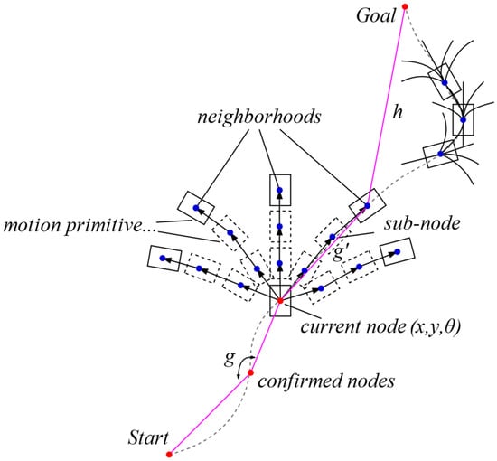
Figure 7. Node expansion with motion primitives (e.g., $N=5, n=3$).

In the HA* algorithm, the node with the lowest cost expands new nodes, where the cost $f$ is calculated using the heuristic functions in Equations (3)–(5):

$$f=g+h={\displaystyle \sum g^{\prime }}+max(h_1,h_2)$$

(3)

$$h_1=l_{db}$$

(4)

$$h_2=l_{pre}$$

(5)

where the cumulative cost $g={\displaystyle \sum g^{\prime }}$ along the path represents the total movement cost from the starting point, with $g^{\prime }$ being the cost of a single-step move; the heuristic cost $h$ measures the distance from the current HA* node $S_k$ to the target and guides the expansion towards it.

The $h_1$ is a heuristic value determined by the length of the shortest Dubins (DB) curve $l_{db}$ from $S_k$ to the target, computed in a one-shot manner without considering obstacles [35]. The DB curve ensures that the terminal segment of the path aligns precisely with the expected position and orientation, enabling seamless and smooth transitions between paths in the topological network. In this study, for simplicity in path length calculation, the length $l_0^{\prime }$ of each segment in the DB curve is set equal to $l_0$, as shown in Table 1. The curvature radius $\gamma$ of the DB curve varies for TSO-HA* and topological planning.

The $h_2$ is another heuristic value that represents the anticipated distance $l_{pre}$ measured from $S_k$ to the target, with obstacles considered. Conventional methods for calculating $h_2$ include the real-time A* search where the A* path length is treated as $l_{pre}$ [36], referred to as A*-dis, and the dynamic programming-based heuristic cost lookup table, known as DP-Map [37]. Experiments show that generating a DP-Map is both time- and storage-intensive, particularly for high-resolution maps, while LDP-Map (Limited DP-Map) constrains Dijkstra’s search space and significantly reduces resource consumption, making it a more suitable candidate for comparison.

However, due to the non-G²-continuity of curvature at the junction between the DB curve and the HA*expansion path, along with the suboptimal heuristic function weight assignment, the paths planned often exhibit redundant turns. To improve path smoothness and better align with actual motion, this study utilizes the coarse-planned HA* waypoints as an initial solution for back-end path optimization. The quasi-Newton method Limited-memory BFGS (L-BFGS) is then employed for path smoothing. Notably, the pre-optimized path lengths are still used as weights in the topological network, which generally suffices for practical applications.

2.5.2. Distance Reference Tree

This study proposes a novel $h_2$ calculation method called the distance reference tree (DRT), which considers planning time, spatial efficiency, and success rate. The DRT integrates A* search and dynamic programming principles. By preplanning the approximately shortest piecewise-linear A* path, the distance $d_i$ from each waypoint $p_i$ of the path to the endpoint (target, $g$) is calculated, and mapped with $p_i$ to create a unique mapping. Each waypoint $p_i$ is stored in a K-dimensional tree (KD-tree) [38,39] to construct the DRT. During the planning process, the K-nearest neighbor (KNN) algorithm is employed to find within the DRT the A* waypoint ($p_0$) closest to the current neighboring node ($S_{k+1}$) and free of collisions. The path distance $d_0$ from $p_0$ to $g$ is then directly obtained from the precomputed mapping, along with the distance $\overline{S_{k+1}{p}_0}$ between neighbors. This provides the approximate shortest distance from $S_{k+1}$ to $g$, which is used as the $h_2$ value. Figure 8 shows the DRT-based h₂ calculation, using a relatively complex scenario for demonstration. This not only maintains generality, but also intuitively expresses the DRT’s logic. The specific process is as follows:

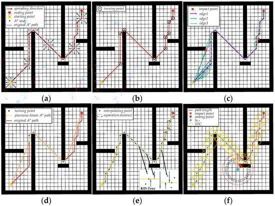
Figure 8. DRT-based h₂ calculation. (a) Eight-neighbor node expansion in A*; (b) turning point extraction; (c) edge construction; (d) approximation of shortest piecewise-linear A* path; (e) interpolation of piecewise-linear A*path and path distance calculation; (f) heuristic value computation.

Step I. As shown in Figure 8a, the initial and final poses are used to construct the original A* path. Given that A* expands nodes in 8 directions, a predefined key-value table <$\theta$-index pairs, fixed-pose> is employed to efficiently expand each new node. This table references the appropriate angle as the pose $\theta$ from the key-value table, based on the row–column index.

Step II. To simplify the original A* path, turning points between consecutive straight-line paths are identified. As shown in Figure 8b, nodes with differing $\theta$-values are extracted from the original A* path and assembled into a new, sparser A* path.

Step III. Linear interpolation is performed on the sparse A* path, followed by the subdivision and interconnection of the interpolation points, as shown in Figure 8c. Passable connections, which do not intersect obstacles, are treated as edges in a weighted directed graph [40]. The length of each edge serving as the Dijkstra weight, with endpoint indexes and connection lengths defining the edge attributes.

Step IV. Dijkstra’s algorithm is used to find the shortest path, resulting in an approximate shortest piecewise-linear A* path, as shown in Figure 8d. This piecewise path connects the starting and ending points more directly than the original A* path, facilitating a more accurate and efficient $d_i$ calculation.

Step V. The piecewise-linear A* path is interpolated at equidistant intervals, and the path distances $d_i$ from each interpolated point $p_i$ to the target $g$ are computed and stored, as shown in Figure 8e. Notably, all grid-based indexes $(X,Y)$ of the interpolated points are stored in a KD-tree as “branch points” to construct the DRT. Each index is linked to its corresponding path distance $d_i$ via a one-to-one mapping. The process for computing $d_i$ is detailed in Algorithm 1. After interpolation, the discretized grid points $(X,Y)$ exhibit significant data volume and uneven distribution. The KD-tree is adopted to organize the row–column indexes of the interpolated points in the approximate A* path as branch points, thereby enhancing the efficiency of querying neighboring nodes $S_{k+1}$ for the nearest A*-interpolated points.

Algorithm 1 Calculating path lengths from “branch points” to the target
Input: waypoints P of the piecewise-linear A* path, interpolation interval δ
Output: interpolation-point(pi) set Φ
1: function GetPointsOnPolyline(P, δ)
2: for i in [0, P.size − 1] do
3:  L ← EuclidDistance(Pi, Pi+1);	▷ Total length of the piecewise-linear A* path.
4: end for
5: Np ← ⌈L/δ⌉;	▷ Number of pi.
6: j ← 0;
7: l ← 0;	▷ LengthMoved.
8: while 0 ≤ i < P·size − 1 and j < Np do
9:  sl ← EuclidDistance(Pi, Pi+1);
10:  while l + δ ≤ sl and j < Np do
11:   ω ← (l + δ)/sl;	▷ Ratio.
12:   Φj·x ← Pi·x + ⌊ω × (Pi+1·x − Pi·x) + 0.5⌋;
13:   Φj·y ← Pi·y + ⌊ω × (Pi+1·y − Pi·y) + 0.5⌋;
14:   Φj·d ← L − (l + δ);	▷ di
15:   l ← l + δ;
16:   j ← j + 1;
17:  end while
18:  L ← L − sl;
19:  l ← l − sl;
20: end while
21: return Φ
22: end function

Step VI. During node expansion, as shown in Figure 8f, the k-nearest neighbor (KNN) algorithm is used to find the closest branch point $p_0$ in the DRT that can establish a collision-free connection with the current node $S_{k+1}$. The distance $\overline{S_{k+1}{p}_0}$ between these two points is retrieved, and the index $(X_n,Y_n)$ is then used for mapping to the precomputed path distance $d_0$, which is added to $\overline{S_{k+1}{p}_0}$ for determining the $h_2$ value of $S_{k+1}$. The process for obtaining each distance is detailed in Algorithm 2 where the Safe Travel Corridor (STC) defined by the distance threshold $d^2$ constrains the node expansion scope.

Algorithm 2 Querying the approximate shortest path length from Sk+1 to the target through DRT
Input: Sk+1 = current node
Require: $\overline{\mathrm{\Phi }}$= an unordered set storing remote and impassable points
Require: pidx = a collection of indexes for ”branch points” on DRT
Require: pD2 = the squared distance from Sk+1 to ”branch points”
Output: h2 = path length from Sk+1 to the ending point
1: function CheckLookUpTable(Sk+1)
2: K ← 1;	▷ K = 1, for the nearest neighbor search algorithm.
3: d2 ← 40 × 40;	▷ 40:the grid distance.
4: δxy ← 0.1	▷ δxy:Spatial resolution of the grid map.
5: loop
6:  if kdtree.nearestKSearch(Sk+1, K, pidx, pD2) > 0 then
7:   for all element i of pidx do
8:    if ${\overline{\mathrm{\Phi }}}_i$=$\overline{\mathrm{\Phi }}$.end then
9:     p0  ← kdtree.getInputCloud ▷ Ψi;	▷ Get the corresponding point in Ψ.
10:     $\overline{S_{k+1}{p}_0}$ ← pD2[i];
11:     if $\overline{S_{k+1}{p}_0}$> d2 then
12:      return h2 ← +∞;	▷ Distance detection.
13:     end if
14:     j← pidx[i];
15:     if not LineHit(Sk+1,p0) then	▷ Collision detection.
16:      h2 ← ($\sqrt{\overline{S_{k+1}{p}_0}}$+ Φj·d0) × δxy
17:      return h2;
18:     else
19:      $\overline{\mathrm{\Phi }}$.insert(j);
20:     end if
21:    end if
22:   end for
23:   K ← K +1;
24:   if K>10 then
25:    return h2 ← +∞;	▷ Overrun.
26:   end if
27:  else
28:    return h2 ← +∞;
29:  end if
30: end loop
31: end function

By simplifying and straightening the original A* path, a reference path with heuristic information is generated to guide the expansion of HA* nodes towards the target.

2.5.3. Occupancy Grid Template

Collision detection is crucial for simulating vehicle impacts with obstacles during node expansion. The traditional HA* algorithm relies on the entire vehicle overlay for accurate collision detection, but significantly increasing computational time. In scenarios with densely distributed waypoints, line collision detection using the vehicle’s contour may be sufficient. Schock and Langlois [41] proposed a relatively precise approach for line collision detection using oriented bounding boxes with heading. Nevertheless, the real-time computation of multiple trigonometric functions in OBBs slows down the planning speed.

In this study, a set of improved occupancy grid templates [42,43] based on the vehicle’s contour are employed for more efficient line collision detection, as shown in Figure 9a. By precomputing the grid coordinates representing the relative row–column offsets from the grid origin, which correspond to the vehicle’s contour in multiple sampling directions with the vehicle’s center at the origin, these coordinates are then compiled into a collision lookup table indexed by orientation ${\theta }_n$, forming the final occupancy grid template, as shown in Figure 9b. The template is generated once before the planning task begins and can be applied to all planning cycles. The method for computing the four vertices $(v{x}_i,v{y}_i)$ of the template is described in Equations (6) and (7):

$$\left\{\begin{array}{l}d{x}_1=cos{\theta }_n\cdot ({\displaystyle \frac{L_0}{2}}+d_0)\\ d{y}_1=sin{\theta }_n\cdot ({\displaystyle \frac{W_0}{2}}+d_0)\\ d{x}_2=sin{\theta }_n\cdot ({\displaystyle \frac{L_0}{2}}+d_0)\\ d{y}_2=-cos{\theta }_n\cdot ({\displaystyle \frac{W_0}{2}}+d_0)\end{array}\right.$$

(6)

$$\left\{\begin{array}{c}(v{x}_1,v{y}_1)=(d{x}_1+d{x}_2,d{y}_1+d{y}_2)\\ (v{x}_2,v{y}_2)=(d{x}_1-d{x}_2,d{y}_1-d{y}_2)\\ (v{x}_3,v{y}_3)=(d{x}_1-d{x}_2,d{y}_1-d{y}_2)\\ (v{x}_4,v{y}_4)=(d{x}_1+d{x}_2,d{y}_1+d{y}_2)\end{array}\right.$$

(7)

where $L_0$ and $W_0$ denote the vehicle’s length and width, respectively, and $d_0$ represents the inflation value used to enlarge the vehicle’s contour and maintain a safety margin.

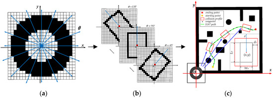
Figure 9. Line collision detection using occupancy grid templates. (a) Set of occupancy grid templates; (b) occupancy grid template for each sampling direction; (c) diagram of collision detection.

The corresponding collision parameters are shown in Table 2. When the rectangular vertices are determined, the grid coordinates can be calculated through the linear interpolation of the connecting lines between vertices. Upon acquiring the precomputed occupancy grid templates, node expansion involves matching the sample angle ${\theta }_n$ closest to the current node’s orientation $\theta$ to retrieve the corresponding grid coordinates. These coordinates are then offset to the node’s position for collision detection by comparing them with the environmental grids at that location, as shown in Figure 9c.

Table 2. Collision parameters.

Parameters	Description	Value
$L_0$	Length of the inspection vehicle	0.72 m
$W_0$	Width of the inspection vehicle	0.58 m
$d_0$	Inflation value or safety distance	0.1 m
$N_{\theta }$	Number of sampling directions for grid templates	72

2.6. Upper-Level Topological Planning

The connection point $C$ is introduced before initiating topological planning on the semi-structured network, which serves to link the starting or ending point with the network, enabling the inspection vehicle to smoothly enter and exit. Specifically, the path segments generated from the starting point to its associated connection points $C_S$ integrate into the semi-structured network, as do the segments originating from the terminal connection points $C_G$ to the target. Connection points are located along directed edges $\overrightarrow{l}$ and are defined as the front or rear pseudo-projection points from the starting or ending point to $\overrightarrow{l}$. The projection point is identified as the waypoint of $\overrightarrow{l}$ closest to the respective starting or ending point, while the front or rear pseudo-projection point represents the waypoint several steps forward or backward from the projection point, based on the orientation of $\overrightarrow{l}$. If the pseudo-projection point extends beyond the boundary of $\overrightarrow{l}$, the beginning waypoint of $\overrightarrow{l}$ is designated as the pseudo-projection point for the starting point, and similarly for the ending point. The number of connection points $\tau$ depends on application requirements. In the context of the caged poultry houses, a single connection point suffices, whereas in more complex environments, $\tau$ can be increased to create a more comprehensive network, aiding in the search for an optimal route. After acquiring the connection points, the TSO-HA* is performed between the connection points $C_S$ and the starting point to derive the connecting paths for integration into the network, as does the process between $C_G$ and the ending point.

In topological planning, a Hash map is employed to manage the collection of waypoints along each path planned using TSO-HA*. The sequential numbers of the initial and final poses for each directed path, including $\overrightarrow{l}$ and $\mathrm{\Omega }$ in Figure 4, serve as the indexes (i.e., keys) in the Hash map. In addition, the sets of waypoints $\mathrm{\Phi }$ from the connection points to the endpoints of $\overrightarrow{l}$, as well as those between the connection points $C_S$ and $C_G$ along the same $\overrightarrow{l}$, as shown in Figure 10, are also indexed. Consequently, by simply providing the initial and final sequence numbers, all waypoints along the path can be accessed.

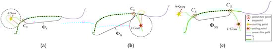
Figure 10. Diagram of connection points. (a) Path planning starting from the starting point to C_S and the corresponding set ${\mathrm{\Phi }}_S$; (b) path planning starting from $C_G$ to the ending point and the corresponding set ${\mathrm{\Phi }}_G$; (c) set ${\mathrm{\Phi }}_{SG}$ between the connection points.

A predetermined cost matrix is maintained by the TSO-HA*-Net for the numerical representation of the semi-structured topological network, with the costs $l$ measured by the TSO-HA* path lengths in Equation (8):

$$l=\left\{\begin{array}{l}{l}_{hastar}=l_{hastar}^{\prime }+l_{db}=M\cdot n\cdot l_0+l_{db}\\ m\cdot n\cdot l_0\end{array}\right.$$

(8)

where the length of the TSO-HA* path is distinguished as follows: in most cases, it is determined by the TSO-HA*-planned path, where $M$ represents the number of TSO-HA* parent nodes, $l_{db}$ denotes the length of the direct DB curve and, $n$ and $l_0$ are shown in Table 1; in cases where the path is planned from the connection points to the corresponding endpoint of $\overrightarrow{l}$, or between the points themselves, it is only a sub-segment of the complete TSO-HA* path, with $m$ representing the number of waypoints in each segment.

Based on the matrix, as shown in Figure 11, Dijkstra’s algorithm is applied to obtain a series of sequence numbers that represent the shortest path between the starting and ending points in the network. The procedure for identifying the minimal-cost path segments is detailed in Algorithm 3. When the sequential indexes representing the shortest path in the network are obtained, the corresponding set of waypoints can be retrieved from the Hash map in order, thereby composing the complete shortest path. The inspection route is derived from this process.

Algorithm 3 Planning the shortest path in the topological network using Dijkstra
Require:  dijnode = the custom node used in Dijkstra containing attributes such as node number node, parent node number prev_node, distance cost cost and comparison function for ascending sorting of distance cost
Data: open_ list = an ordered set of dijnode sorted in ascending order by node cost
Data: close_ list = a collection of dijnode storing processed nodes
Result: idxes = sequence numbers (label) of the shortest path
1: function DIJKSTRA( )
2: open_ list.insert(dijnode {0, 0, 0.0});		▷ Insert the starting point into open_ list as the initial node.
3: repeat
4: node_ ← open_list.extract(open_list.begin);		▷ Extract the first element from open_list.
5:  if node_.node = 1 then		▷ 1 is the number of the end, which means open_list is complete.
6:   while node_.prev_node ≠ 0 do		▷ 0: the number of the start./Backtracking the path.
7:    idxes.insert(node_.node);
8:    for all element a of close_ list do
9:     if a.node = node_ .prev_node then		▷ The parent node of the current node exists.
10:      node_ ← a;		▷ Update.
11:     else
12:      ERROR: No whole path. Stop while.
13:     end if
14:    end for
15:   end while
16:   idxes.insert(node_.node);		▷ This is the child node of the starting point.
17:   reverse_path(idxes.begin, idxes.end);		▷ Reversing the path.
18:   Stop repeat.;
19:  end if //Now look for the shortest path.
20:  close_list.insert(node_);		▷ Points placed in close_list will no longer be processed.
21:  for i in [0, node_num) do		▷ node_num: predefined number of network nodes.
22:   if i = node_.node then		▷ The current node.
23:    Next for;
24:   end if
25:   for all element a of close_ list do
26:    if a.node = i then		▷ The node is in close_ list.
27:     Next for-21;
28:    end if
29:   end for
30:   if graph_ [node_.node][i] = +∞ then	▷ graph_: cost matrix indexed by waypoints’ label.
31:    Next for;	▷ Ignore nodes with infinite cost.
32:   end if	▷ The node with the least cost so far.
33:   dijnode: open_node{i, node_.node, node_ .cost + graph_ [node_.node][i]};
34:   for all element b of open_ list do
35:    if b.node = open_node.node then	▷ Identical label.
36:     ifb.cost > open_node.cost then	▷ The cost in open_list is too large.
37:      open_list.erase(b);	▷ Update.
38:      open_list.insert(open_node);
39:     end if
40:    else
41:     open_ list.insert(open_node);
42:     end if
43:    end for
44:   end for
45:  until open_ list.empty
46:  return idxes
47: end function

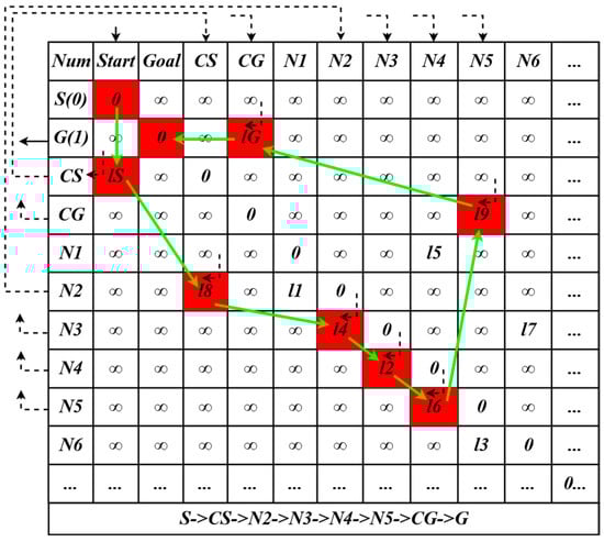
Figure 11. Diagram of the cost matrix ($\tau =1$).

3. Result and Discussion

This study conducts comparative experiments of global path planning based on several algorithms using the Jetson Orin NX 8GB with an Arm Cortex A78AE 6-core CPU, running the Ubuntu 20.04LTS operating system and ROS Noetic meta-operating system. Rviz 1.14.17 is utilized as the visualization interface.

3.1. h₂ Calculation

Given the same initial and final poses, as well as the identical node-expansion parameters, the DB curve settings shown in Table 1, the back-end optimization method described in Section 2.5.1, and the collision detection method detailed in Section 2.5.3, the TSO-HA* planning results for six different scenes within the poultry houses are obtained using DRT, described in Section 2.5.2. As shown in Figure 12, the TSO-HA* algorithm generates collision-free, smooth paths with short distances and curvature constraints, requiring only the specification of initial and final poses.

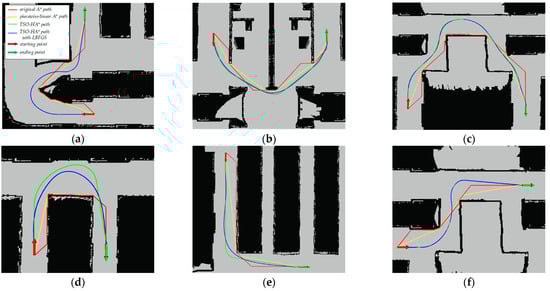
Figure 12. Planning results using DRT. (a–f) Scene I–VI within the poultry houses, respectively.

To minimize variability, multiple planning runs are performed for each scene, and the average results using DRT in TSO-HA*, LDP-MAP, and A*-dis are shown in Table 3. The DRT method achieves a planning success rate close to 100% and demonstrates exceptional robustness across various scenes, significantly outperforming LDP-MAP, which has a success rate of 83.3%, and A*-dis, which achieves only 50%. The DRT method benefits from a more valuable lookup table, ensuring the optimal utilization of pre-stored nodes, whereas LDP-MAP results in the accumulation of redundant stored nodes and inefficient utilization. Despite minor variations in path lengths across the three algorithms, TSO-HA* consistently guarantees asymptotically optimal path lengths. Summaries of temporal and spatial performance for the three algorithms are shown in Figure 13, which indicate that TSO-HA* achieves shorter computation time, reduced resource consumption, and a higher success rate when applied to high-resolution maps.

Table 3. Summary of experimental results for the three algorithms.

Algorithm (Success Rate/%)	Scene	Time for Lookup Table [a]		Time for Front-End Planning		Time for Back-End Optimization		Planning Time /ms	Total Time /ms	Number of Stored Nodes [b]	Number of Explored Nodes [c]	Value Ratio [d]/%	Path Length [e] /m
		ms	%	ms	%	ms	%
DRT (100%)	I	415.7	28.43	655.7	44.85	390.7	26.72	1046.4	1462.1	86	2683	3119.77	30.63
	II	927.0	19.44	3359.4	70.44	482.6	10.12	3842.0	4768.9	96	11,740	12,229.17	30.27
	III	1349.4	19.61	4809.1	69.90	721.1	10.48	5530.3	6879.8	136	15,230	11,198.53	45.17
	IV	420.2	38.18	50.3	8.57	630.1	57.25	680.5	1100.6	67	142	211.95	25.91
	V	912.1	44.65	31.3	1.53	1099.4	53.82	1130.7	2042.8	124	99	79.84	38.97
	VI	93.1	20.61	62.6	13.85	295.9	65.54	358.5	451.5	84	217	258.33	28.71
LDP-MAP (83.3%)	I	2582.1	72.29	632.1	17.70	357.7	10.01	989.8	3571.9	32,689	2703	8.27	31.09
	II	5241.4	48.14	5118.9	47.01	528.3	4.85	5647.2	10,888.6	60,537	21,580	35.65	30.44
	III	1605.3	−	− [f]						19,327	−
	IV	2344.1	86.45	68.3	2.52	299.1	11.03	367.5	2711.5	31,965	491	1.54	23.23
	V	6238.1	93.81	25.2	0.38	386.5	5.81	411.7	6649.8	74,706	88	0.12	37.68
	VI	3664.4	89.36	66.7	1.62	369.8	9.02	436.5	4100.9	44,461	240	0.54	28.67
A*-dis (50%)	I–III	0		−
	IV			26,115.6	97.78	591.7	2.22	26,706.8	26,706.8	3036 [g]	153	−	25.92
	V			37,893.1	96.52	1366.5	3.48	39,259.6	39,259.6	6213	99		39.32
	VI			27,814.1	97.01	858.1	2.99	28,672.2	28,672.2	2413	251		28.95

Note: [a] Both the DRT and LDP-MAP methods require pre-generated h₂-value lookup tables; [b] static storage resources used to record h₂ before the planning, i.e., DRT branch points or LDP-MAP grids; [c] dynamic storage resources used to obtain h₂ during the planning; [d] percentage of explored nodes relative to stored nodes, reflecting the reference value of the lookup table; [e] HA* path length without back-end optimization; [f] planning failure is defined as planning time exceeding 50 s; [g] average number of nodes used for A* search within one planning cycle.

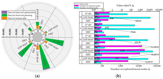
Figure 13. Summaries of temporal and spatial performance across the three algorithms. (a) Temporal summary; (b) spatial summary.

The LDP-MAP requires more time to construct the lookup table, with an average increase in table-generation time of 74.5%, and a minimum increase of 15.9% compared to DRT in this study. In contrast, DRT achieves an average reduction in total time of 66.6%, with a minimum reduction of 56.2% compared to LDP-MAP, and an average time decrease of 96.4% compared to A*-dis. Furthermore, fewer nodes are used in DRT to assist in the h₂ calculation due to its reliable lookup table, the average number of stored nodes is reduced by 99.7% compared to LDP-MAP, and the average numbers of stored and explored nodes are reduced by 97.4% and 6.9%, respectively, compared to A*-dis. The results show that the DRT method employed by TSO-HA* is the most time- and space-efficient for h₂ calculation across various planning scenes.

As shown in Table 4, a computational complexity analysis is conducted to further validate the performance of DRT despite variations in the experimental environment. Due to the large number of stored nodes used in LDP-MAP and A*-dis presented in Table 3, the overall analysis demonstrates that the DRT method has the lowest time and space complexity, verifying its low computational time and memory usage.

Table 4. Computational complexity analysis.

Algorithm	Lookup Table Construction		Single Node Exploration [b]
	Time Complexity [a]	Space Complexity	Time Complexity	Space Complexity
DRT	$O(n+N)$ [c]	$O(n+N)$	$O(logN)$	$O(N)$
LDP-MAP	$O(N\cdot logN)$	$O(N)$	$O(1)$	$O(1)$
A*-dis	−		$O(N\cdot logN)$	$O(N)$

Note: [a] Worst-case time complexity; [b] computational complexity analysis of expanding one node, with the total number of explored nodes shown in Table 3; [c] n represents the number of nodes in the piecewise-linear A* path (typically small), and N is the number of stored nodes shown in Table 3.

3.2. Line Collision Detection

Under unified planning points and scenarios, and utilizing the same h₂ calculation method described in Section 2.5.2, collision detection experiments are conducted using the collision parameters listed in Table 2 with the occupancy grid template (OGT) and the oriented bounding box (OBB). As shown in Table 5, using the pre-existing occupancy grid templates results in only 2592 collision grid storage consumption and an average template-generation time of 0.78 ms, in comparison to the OBB. However, the front-end planning time is decreased by at least 4.0%, with an average reduction of 22.6%. This finding indicates that the use of occupancy grid templates significantly enhances planning speed while incurring only a minimal static memory overhead.

Table 5. Results with different collision-detection algorithms.

Algorithm	Scene	Time for Template /ms	Time for Front-End Planning /ms	Time Reduction in Front-End Planning		Detection Mode	Number of Stored Collision Grids [a]
				ms	%
OGT (TSO-HA* used)	I	0.78 [b]	655.71 [c]	670.81	50.6	Template matching	2592
	II		3359.40	1289.71	27.7
	III		4809.19	1148.06	19.3
	IV		50.33	2.08	4.0
	V		31.31	7.53	19.4
	VI		62.55	10.49	14.4
OBB	I	0	1326.52	−		Real-time computation	0
	II		4649.11
	III		5957.25
	IV		52.41
	V		38.84
	VI		73.04

Note: [a] The grid template is statically pre-stored with collision grids retrieved during node expansion; [b] since the total number of grids is fixed and the template-generation time is similar, the average value is taken here; [c] as the experiment is based on identical conditions, the planning time here is the same as that in Table 3.

Furthermore, integrating collision detection into the original A* path of DRT, referred to as prior collision detection, helps prevent the piecewise-linear A* path from being obstructed in impassable narrow passages. This approach thereby avoids planning failures, as shown in Figure 14.

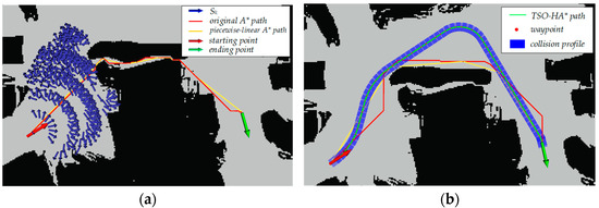
Figure 14. Planning effects with and without prior collision detection. (a) Planning gets stuck in the narrow passage; (b) planning escapes from the narrow passage.

The experimental results before and after implementing prior collision detection, using occupancy grid templates as an example, are shown in Table 6. The results show that the incorporation of prior collision detection leads to a marginal average increase of 1.9% in node storage and 1.8% in node exploration, respectively. The maximum observed increments are 4.7% for node storage and 4.8% for exploration. Additionally, the average generation time for the lookup table is increased by 274.08 ms. However, the total time decreased by an average of 332.64 ms, representing a reduction of 19.1%. The results show that, despite the slight increase in table-generation time and node storage, the integration of prior collision detection improves the distribution rationality of the stored nodes, thus accelerating the planning process.

Table 6. Performance comparison with prior collision detection.

Scene	Time Rise in Lookup Table		Time Rise in Front-End Planning		Reduction in Total Time		Rise in the Number of Stored Nodes		Rise in the Number of Explored Nodes
	ms	%	ms	%	ms	%		%		%
I	203.47	49.0	153.09	23.3	34.16	2.3	4	4.7	129	4.8
II	398.63	43.0	−249.17	−7.4	333.13	7.0	1	1.0	37	0.3
III	506.52	37.5	80.69	1.7	133.92	1.9	1	0.7	319	2.1
IV	62.60	14.9	−7.63	−15.2	575.16	52.3	2	3.0	3	2.1
V	217.27	23.8	−2.05	−6.5	884.17	43.3	1	0.8	0	0.0
VI	255.98	275.1	4.59	7.3	35.34	7.8	1	1.2	3	1.4
Mean	274.08	73.9	−		332.64	19.1	1.7	1.9	81.8	1.8
Min. (Max.)	506.52	275.1			34.16	1.9	4	4.7	319	4.8

3.3. Planning Inspection Routes Based on TSO-HA*-Net

The TSO-HA* algorithm, leveraging the distance reference tree and occupancy grid templates, achieves a significant reduction in both the time and spatial consumption required for path planning. This enhancement is crucial for improving the speed, efficiency, and success rate of constructing the semi-structured topological network and inspection routes. Based on the edge connectivity depicted in Figure 4, a semi-structured topological network is constructed using the TSO-HA* algorithm, as shown in Figure 15a. Subsequently, topological planning is conducted based on this network. Figure 15b demonstrates how the planned path is constrained by the topological network and relies on the connection points to merge seamlessly into the network. These connection points (indicated by labels 2 and 3 in Figure 15b) are key components in constructing the complete network, and serve as critical points for the inspection vehicle to enter and exit the network.

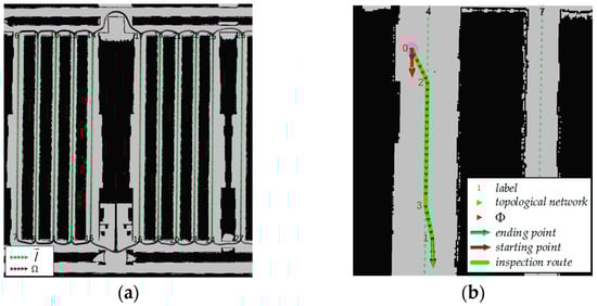
Figure 15. Semi-structured topological network. (a) Network construction; (b) merging the path into the network.

Planning inspection routes using TSO-HA*-Net demonstrates outstanding planning performance. In Figure 16a, pathways through elongated inter-cage corridors maintain linear trajectories, while “U”-shaped intersections exhibit seamless connectivity and smooth transitions. This both helps mitigate tire wear and motor strain caused by stationary rotations in the differential-drive inspection vehicle, and complies with the Ackermann steering geometry. By extracting key waypoints from linear path segments at regular intervals and storing them in a KD-tree format, detection points are designated where inspection vehicles can stop to identify diseased or dead poultry. Figure 16b illustrates that the inspection route retains the capability to cover specific areas, indicating that the inspection vehicle can reach designated locations such as charging stations and maintenance areas via the shortest path while adhering to the constraints of the topological network. Collectively, these findings demonstrate that the inspection route designed by the TSO-HA*-Net algorithm not only continuously covers the corridors within the poultry house, but also ensures optimal and shortest path characteristics. This enables the inspection vehicle to follow a fixed work route while retaining the flexibility to reach specific locations through the shortest path. The TSO-HA*-Net algorithm thus successfully establishes a compromise between point-to-point path planning and full-coverage path planning, systematically addressing the inspection route requirements for the poultry houses and aligning with the actual environment. Moreover, the planned route enables house-to-house inspection, as shown in Figure 17, reducing the need for additional vehicles.

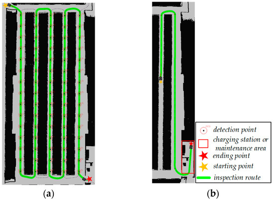
Figure 16. Single-house topological planning. (a) Inspection route; (b) access to specific positions.

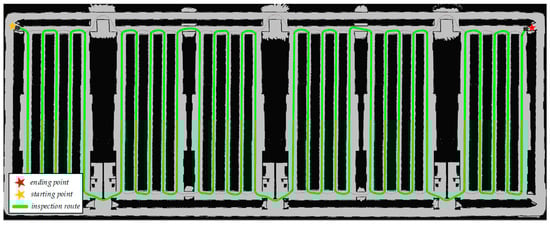
Figure 17. Multiple-house topological planning.

The TSO-HA*-Net algorithm efficiently reduces the computational time required for both single-house and multiple-house topological planning. Planning an inspection route for a single house takes an average of 257.98 ms, while planning the global route that involves cross-coop transfers requires only 546.62 ms. These results fully demonstrate the efficiency of the algorithm, making it particularly suitable for the continuous, flexible, and rapid planning of inspection routes on large-scale, high-resolution grid maps.

Furthermore, depending on the semi-structured network via TSO-HA*-Net, coordinated inspections by multiple vehicles across single or multiple houses can be realized, enhancing inspection efficiency in large-scale poultry farming, as shown in Figure 18. This capability ensures the synchronization and stability of inspection operations, thereby providing technical support for the efficient management of modern poultry farming.

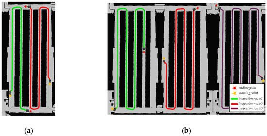
Figure 18. Multi-vehicle collaboration planning. (a) Within a single house; (b) across multiple houses.

4. Conclusions

Track-based inspection schemes face challenges such as track disconnection, contamination, and high installation and maintenance costs, while current rail-less solutions lack stable and reliable path planners. To address these issues, we propose a hybrid global path planner TSO-HA*-Net, which combines the spatiotemporally optimized Hybrid A* (TSO-HA*) algorithm with topological planning. The TSO-HA* incorporates an enhanced node expansion strategy, the distance reference tree, and simplified occupancy grid templates. Topological planning is adopted to find the shortest path within the network via connection points to derive an inspection route.

The experiments conducted in poultry houses show the time- and space-efficiency of the TSO-HA* algorithm. Compared to LDP-MAP and A*-dis, the total planning time of the TSO-HA* utilizing the DRT for h₂ calculation is reduced by 66.6% and 96.4%, respectively, and the number of stored nodes is decreased by 99.7% and 97.4%, respectively. TSO-HA*-Net is efficient and flexible for planning inspection routes in caged poultry houses, requiring only 546.62 ms for a single global route. A balanced planning approach between point-to-point and full-coverage path planning is established, meeting the route requirements for coop inspection while adapting to the actual poultry house environment. The proposed planner can generate a continuous and complete route within a single planning process and serve as a foundational tool for facilitating cross-regional and multi-vehicle inspections. This innovation fills the gap in the inspection vehicle’s lack of a reliable global planner.

Future work will focus on integrating localization and navigation capabilities. By building on existing localization techniques, translating waypoints into trajectories, and employing control algorithms such as MPC, inspection task execution can be truly fulfilled. Additionally, nearest neighbor search algorithms will be used for precise localization to track the cage location of abnormal poultry.

References

- Jin, Y.C.; Liu, J.Z.; Xu, Z.J.; Yuan, S.Q.; Li, P.P.; Wang, J.Z. Development Status and Trend of Agricultural Robot Technology. Int. J. Agric. Biol. Eng. 2021, 14, 1–19. [Google Scholar] [CrossRef]
- Vroegindeweij, B.A.; Blaauw, S.K.; Ijsselmuiden, J.M.M.; van Henten, E.J. Evaluation of the performance of PoultryBot, an autonomous mobile robotic platform for poultry houses. Biosyst. Eng. 2018, 174, 295–315. [Google Scholar] [CrossRef]
- Liu, H.W.; Chen, C.H.; Tsai, Y.C.; Hsieh, K.W.; Lin, H.T. Identifying Images of Dead Chickens with a Chicken Removal System Integrated with a Deep Learning Algorithm. Sensors 2021, 21, 3579. [Google Scholar] [CrossRef] [PubMed]
- Zhao, Y.; Shepherd, T.A.; Swanson, J.C.; Mench, J.A.; Karcher, D.M.; Xin, H. Comparative evaluation of three egg production systems: Housing characteristics and management practices. Poult. Sci. 2015, 94, 475–484. [Google Scholar] [CrossRef]
- Ren, G.; Lin, T.; Ying, Y.; Chowdhary, G.; Ting, K.C. Agricultural robotics research applicable to poultry production: A review. Comput. Electron. Agric. 2020, 169, 105216. [Google Scholar] [CrossRef]
- Zheng, H.; Li, B.; Chen, G.; Wang, C. Improving utilization of nests and decreasing mislaid eggs with narrow width of group nests. Int. J. Agric. Biol. Eng. 2018, 11, 83–87. [Google Scholar] [CrossRef]
- Hao, H.; Fang, P.; Duan, E.; Yang, Z.; Wang, L.; Wang, H. A Dead Broiler Inspection System for Large-Scale Breeding Farms Based on Deep Learning. Agriculture 2022, 12, 1176. [Google Scholar] [CrossRef]
- Wu, D.; Cui, D.; Zhou, M.; Ying, Y. Information perception in modern poultry farming: A review. Comput. Electron. Agric. 2022, 199, 107131. [Google Scholar] [CrossRef]
- Shi, Z.; Hao, Z.; Teng, G.; Xiong, J.; Zhao, Y.; Ye, B. Dead Chicken Polling Device and Dead Chicken Polling Method for Three-Dimensional Chicken-Raising System. CN Patent Application CN109729998A; CN109729998B, 26 November 2018. (In Chinese with English Abstract). [Google Scholar]
- Hartung, J.; Lehr, H.; Domenech, D.R.; Mergeay, M.; van den Bossche, J. ChickenBoy: A farmer assistance system for better animal welfare, health and farm productivity. In Proceedings of the 9th European Conference on Precision Livestock Farming (ECPLF), Cork, Ireland, 26–29 August 2019; pp. 272–276. [Google Scholar]
- Feng, Q.; Wang, B.; Zhang, W.; Li, X. Development and Test of Spraying Robot for Anti-epidemic and Disinfection in Animal Housing. In Proceedings of the 2021 WRC Symposium on Advanced Robotics and Automation (WRC SARA), Beijing, China, 11 September 2021; pp. 24–29. [Google Scholar]
- Li, L.; Xing, L.; Duan, Q. Design and implementation of unmanned patrol system for large-scale chicken house. Heilongjiang Anim. Sci. Vet. Med. 2021, 3, 58–62+66+159. [Google Scholar]
- Liu, H.; Yan, S.C.; Shen, Y.; Li, C.H.; Zhang, Y.F.; Hussain, F. Model Predictive Control System Based on Direct Yaw Moment Control for 4WID Self-steering Agriculture Vehicle. Int. J. Agric. Biol. Eng. 2021, 14, 175–181. [Google Scholar] [CrossRef]
- Zhang, Y.Y.; Zhang, B.; Shen, C.; Liu, H.L.; Huang, J.C.; Tian, K.P.; Tang, Z. Review of the Field Environmental Sensing Methods Based on Multi-sensor Information Fusion Technology. Int. J. Agric. Biol. Eng. 2024, 17, 1–13. [Google Scholar]
- Neethirajan, S. ChickTrack—A quantitative tracking tool for measuring chicken activity. Measurement 2022, 191, 110819. [Google Scholar] [CrossRef]
- Vroegindeweij, B.A.; Ijsselmuiden, J.M.M.; van Henten, E.J. Probabilistic localization in repetitive environments: Estimating a robot’s position in an aviary poultry house. Comput. Electron. Agric. 2016, 124, 303–317. [Google Scholar] [CrossRef]
- Li, M.H.; Gao, H.Y.; Zhao, M.X.; Mao, H.P. Development and Experimentation of a Real-Time Greenhouse Positioning System Based on IUKF-UWB. Agriculture 2024, 14, 1479. [Google Scholar] [CrossRef]
- Lu, E.; Ma, Z.; Li, Y.M.; Xu, L.Z.; Tang, Z. Adaptive Backstepping Control of Tracked Robot Running Trajectory Based on Real-time Slip Parameter Estimation. Int. J. Agric. Biol. Eng. 2020, 13, 178–187. [Google Scholar] [CrossRef]
- Peng, Z. Research on SLAM and Navigation Technology of Indoor Mobile Robot Based on ROS in Poultry Farm. Master’s Thesis, South China Agricultural University, Guangzhou, China, 2019. [Google Scholar]
- Li, M. Research on Navigation and Motion Control Method of Inspection Robot in Chicken Houses. Master’s Thesis, North University of China, Taiyuan, China, 2021. [Google Scholar]
- Zhang, Y. Two-Wheeled Autonomously Controlled Chicken Coop Inspection Robot Path Planning Research. Master’s Thesis, North University of China, Taiyuan, China, 2023. [Google Scholar]
- Han, Y.; Li, S.; Wang, N.; An, Y.; Zhang, M.; Li, H. Detecting center line of chicken coop path using 3D Lidar. Trans. Chin. Soc. Agric. Eng. 2024, 40, 173–181. [Google Scholar]
- Yang, D.; Cui, D.; Ying, Y. Development and trends of chicken farming robots in chicken farming tasks: A review. Comput. Electron. Agric. 2024, 221, 108916. [Google Scholar] [CrossRef]
- Yarovoi, A.; Cho, Y.K. Review of simultaneous localization and mapping (SLAM) for construction robotics applications. Autom. Constr. 2024, 162, 105344. [Google Scholar] [CrossRef]
- Mangelson, J.G.; Dominic, D.; Eustice, R.M.; Vasudevan, R. Pairwise Consistent Measurement Set Maximization for Robust Multi-Robot Map Merging. In Proceedings of the 2018 IEEE International Conference on Robotics and Automation (ICRA), Brisbane, QLD, Australia, 21–25 May 2018; pp. 2916–2923. [Google Scholar]
- Yin, P.; Zhao, S.; Lai, H.; Ge, R.; Zhang, J.; Choset, H.; Scherer, S. AutoMerge: A Framework for Map Assembling and Smoothing in City-Scale Environments. IEEE Trans. Robot. 2023, 39, 3686–3704. [Google Scholar] [CrossRef]
- Zheng, H.; Dai, M.; Zhang, Z.; Xia, Z.; Zhang, G.; Jia, F. The Navigation Based on Hybrid A Star and TEB Algorithm Implemented in Obstacles Avoidance. In Proceedings of the 2023 29th International Conference on Mechatronics and Machine Vision in Practice (M2VIP), Queenstown, New Zealand, 21–24 November 2023; Volume 2, pp. 1–6. [Google Scholar]
- Xue, W.; Ying, R.; Gong, Z.; Miao, R.; Wen, F.; Liu, P. SLAM Based Topological Mapping and Navigation. In Proceedings of the IEEE/ION Position, Location and Navigation Symposium (PLANS), Portland, OR, USA, 20–23 April 2020; pp. 1336–1341. [Google Scholar]
- Dolgov, D.; Thrun, S.; Montemerlo, M.; Diebel, J. Practical Search Techniques in Path Planning for Autonomous Driving. In AAAI Workshop-Technical Report; AAAI: Washington, DC, USA, 2008. [Google Scholar]
- Dolgov, D.; Thrun, S.; Montemerlo, M.; Diebel, J. Path Planning for Autonomous Vehicles in Unknown Semi-structured Environments. Int. J. Robot. Res. 2010, 29, 485–501. [Google Scholar] [CrossRef]
- Shamsudin, A.U.; Ohno, K.; Hamada, R.; Kojima, S.; Mizuno, N.; Westfechtel, T.; Suzuki, T.; Tadokoro, S.; Fujita, J.; Amano, H. Two-stage Hybrid A* path-planning in large petrochemical complexes. In Proceedings of the 2017 IEEE International Conference on Advanced Intelligent Mechatronics (AIM), Munich, Germany, 3–7 July 2017; pp. 1619–1626. [Google Scholar]
- Sedighi, S.; Nguyen, D.V.; Kapsalas, P.; Kuhnert, K.D. Implementing Voronoi-based Guided Hybrid A* in Global Path Planning for Autonomous Vehicles. In Proceedings of the 2019 IEEE Intelligent Transportation Systems Conference (ITSC), Auckland, New Zealand, 27–30 October 2019; pp. 3845–3852. [Google Scholar]
- Zhang, S.; Jian, Z.; Deng, X.; Chen, S.; Nan, Z.; Zheng, N. Hierarchical Motion Planning for Autonomous Driving in Large-Scale Complex Scenarios. IEEE Trans. Intell. Transp. Syst. 2022, 23, 13291–13305. [Google Scholar] [CrossRef]
- Hart, P.E.; Nilsson, N.J.; Raphael, B. A Formal Basis for the Heuristic Determination of Minimum Cost Paths. IEEE Trans. Syst. Sci. Cybern. 1968, 4, 100–107. [Google Scholar] [CrossRef]
- Dubins, L.E. On curves of minimal length with a constraint on average curvature and with prescribed initial and terminal positions and tangents. Am. J. Math. 1957, 79, 497–516. [Google Scholar] [CrossRef]
- Kurzer, K. Path Planning in Unstructured Environments: A Real-time Hybrid A* Implementation for Fast and Deterministic Path Generation for the KTH Research Concept Vehicle. Master’s Thesis, KTH Stockholm, Stockholm, Sweden, 2016. [Google Scholar]
- Petereit, J.; Emter, T.; Frey, C.W.; Kopfstedt, T.; Beutel, A. Application of Hybrid A* to an Autonomous Mobile Robot for Path Planning in Un-structured Outdoor Environments. In Proceedings of the ROBOTIK 2012. In Proceedings of the 7th German Conference on Robotics, Munich, Germany, 21–22 May 2012; pp. 1–6. [Google Scholar]
- Hu, L.; Nooshabadi, S.; Ahmadi, M. Massively parallel KD-tree construction and nearest neighbor search algorithms. In Proceedings of the 2015 IEEE International Symposium on Circuits and Systems (ISCAS), Lisbon, Portugal, 24–27 May 2015; pp. 2752–2755. [Google Scholar]
- Hou, W.; Li, D.; Xu, C.; Zhang, H.; Li, T. An Advanced k Nearest Neighbor Classification Algorithm Based on KD-tree. In Proceedings of the 2018 IEEE International Conference of Safety Produce Informatization (IICSPI), Chongqing, China, 10–12 December 2018; pp. 902–905. [Google Scholar]
- Ammar, A.; Bennaceur, H.; Châari, I.; Koubâa, A.; Alajlan, M. Relaxed Dijkstra and A* with Linear Complexity for Robot Path Planning Problems in Large-Scale Grid Environments. Soft Comput. 2016, 20, 4149–4171. [Google Scholar] [CrossRef]
- Schock, A.; Langlois, R.G. Continuous Appropriately-Oriented Collision Detection Algorithm for Physics-Based Simulations. In Proceedings of the 9th International Conference of Control Systems, and Robotics (CDSR’22), Niagara Falls, ON, Canada, 2–4 June 2022. [Google Scholar]
- Ziegler, J.; Werling, M. Navigating car-like robots in unstructured environments using an obstacle sensitive cost function. In Proceedings of the 2008 IEEE Intelligent Vehicles Symposium, Eindhoven, The Netherlands, 4–6 June 2008; pp. 787–791. [Google Scholar]
- Amanatides, J.; Woo, A. A Fast Voxel Traversal Algorithm for Ray Tracing. Eurographics 1987, 87, 1017–4656. [Google Scholar]
Disclaimer/Publisher’s Note: The statements, opinions and data contained in all publications are solely those of the individual author(s) and contributor(s) and not of MDPI and/or the editor(s). MDPI and/or the editor(s) disclaim responsibility for any injury to people or property resulting from any ideas, methods, instructions or products referred to in the content. |
© 2025 by the authors. Licensee MDPI, Basel, Switzerland. This article is an open access article distributed under the terms and conditions of the Creative Commons Attribution (CC BY) license (https://creativecommons.org/licenses/by/4.0/).