Precise Humidity Regulation for Grafted Seedling Plant Factories Based on Quadratic Regression Modeling and Machine Learning Prediction

Abstract

This paper presents a valve-controlled pipeline humidification system aimed at achieving precise and uniform humidity regulation in the multi-layer cultivation environments of plant factories. Since grafted seedlings require stable humidity conditions for effective healing, the system was designed to enable fine-grained adjustments across different cultivation layers. A quadratic regression orthogonal rotational combination design was employed to investigate how valve opening angles affect mean relative humidity (MRH), and a regression prediction model was developed accordingly. The model exhibited strong predictive performance, achieving an R² of 0.9907 and an average relative error of only 0.67%. The optimal valve-opening angles were 60°, 50°, and 50°, respectively, which ensured that the MRH remained above 90% throughout operation. Experimental verification confirmed that the model accurately predicted humidity responses, while the proposed system improved uniformity by reducing the humidity variation from 6.1% to 0.3% and increasing the compliance rate from 58.3% to 100%. To enhance short-term humidity forecasting, three machine learning algorithms—Random Forest, XGBoost, and Transformer—were trained to predict humidity trends within a 6-h window. Among them, the RF model achieved the highest accuracy with an R² of 0.9543, outperforming the other models in both stability and precision. The main contribution of this study is the identification of the optimal valve-opening combination through a quadratic orthogonal rotation regression combination experiment. Additionally, the RF obtained the optimal machine learning model for predicting humidity within 6 h.

1. Introduction

Plant factories represent fully enclosed, climate-controlled cultivation systems that enable continuous, year-round vegetable production without external environmental fluctuations [1,2,3]. Through the integration of artificial lighting and precise environmental regulation, these facilities maintain stable growth conditions that ensure high productivity and uniform crop quality [4,5]. Compared with conventional greenhouses, plant factories demonstrate superior resource efficiency, reduced pesticide dependency, and shortened production cycles [6]. In particular, the controlled environment provides optimal conditions for grafted seedlings, reducing pathogen pressure, improving graft union success rates, and thus supporting large-scale and standardized seedling propagation [7].

With intensifying urbanization and arable land decline, controlled environment agriculture has emerged as a key strategy in sustainable food production [8]. Seeds and seedlings cultivated under CEA systems exhibit enhanced physiological quality, accelerated growth, and increased yield stability [9]. Within such systems, vegetable grafting has become an indispensable technology enabling high-density and year-round cultivation [10]. Grafting was originally developed in East Asia to address soil-borne diseases and environmental stresses. Today, it is widely used to grow solanaceous and cucurbit crops under LED lighting, combining disease-resistant rootstocks with high-quality scions [11]. However, the grafting process requires precise microclimate control, especially relative humidity, because excessive transpiration during the early healing stage can dry out the graft union and prevent proper callus formation [12,13]. It is therefore necessary to keep the humidity within an appropriate, optimal range (90–95% RH).

Maintaining an optimal RH environment is therefore crucial for successful graft healing and acclimatization. Conventional humidification methods in plant factories—such as ultrasonic foggers, high-pressure sprays, and thermal vapor generators—can maintain relative humidity levels above 85%; however, each has its own limitations. Ultrasonic atomization often causes local oversaturation and uneven humidity distribution [14]. High-pressure systems are expensive and require frequent maintenance [15], while thermal vapor systems raise both temperature and energy consumption beyond the optimal graft development range [16]. To address these limitations, a valve-controlled pipeline humidification system was developed, enabling precise humidity regulation via adjustable valve flow control.

To optimize system performance and capture the nonlinear interactions between valve opening and relative humidity, a quadratic regression modeling approach was adopted. Originally applied in industrial process optimization, such models have proven effective in describing multidimensional relationships and determining optimal control parameters in agricultural and environmental systems [17,18,19,20,21]. Previous studies, such as those conducted by Rong et al. [22] and Wang et al. [23], successfully used second-order regression models to analyze interactions among multiple factors in soil improvement and machine optimization. These studies highlight the potential of this approach for developing adaptive and energy-efficient environmental control systems in plant factories.

Furthermore, machine learning models have become increasingly valuable for environmental prediction and system optimization. Rezaei Melal et al. [24] and Wei et al. [25]. conducted humidity prediction studies in which multiple machine learning models were compared to identify the optimal model for final training. Their selected models achieved high R² values and low prediction errors, providing a useful reference for the present work. Qin et al. [26] further reported that the XGBoost model produced an R² value for humidity prediction that was 0.07 higher than that for temperature, and its RMSE, MAE, and MAPE metrics were also superior to those obtained for temperature prediction.

Qadeer Kinza et al. [27] demonstrated that the Random Forest model achieved superior accuracy in humidity prediction compared to Support Vector Machines in air-based energy management systems. Similarly, Sarkar Himangshu et al. [28] and Sun Kailai et al. [29] showed that XGBoost- and Transformer-based algorithms outperform conventional models in hydrological and occupancy prediction tasks, respectively. Drawing on these advances, this study employed RF, XGBoost, and Transformer models to predict RH dynamics within grafted seedling plant factories, aiming to identify the most accurate and efficient predictive framework.

This article uses a quadratic regression orthogonal rotation combination design experiment to obtain the optimal valve opening, ensuring that the cultivation space on different shelf levels can achieve the target humidity. In addition, this study also predicts the humidity changes within 6 h through machine learning, proposing the optimal humidity prediction model by comparing RF, XGBoost, and Transformer models. It provides a fundamental understanding for maintaining high-humidity environments in plant factories with multiple cultivation rack layers.

2. Materials and Methods

2.1. Experimental Materials

The plant factory is located at the Institute of Facility Agriculture, Guangdong Academy of Agricultural Sciences (IFA, GDAAS), at coordinates 23°8′51.9″ N, 113°21′39.03″ E. This independently developed controlled environment chamber features artificial lighting, a multi-functional refrigeration system, piped humidification devices, and four cultivation shelves. The facility dimensions are 2880 mm (L) × 1840 mm (W) × 2260 mm (H), with 100 mm thick insulated panels. Each cultivation shelf measures 1235 mm (L) × 605 mm (W) × 1790 mm (H). Adjustable LED panels emitting white, red, and purple light are mounted above each cultivation bed. Pipelines installed 150 mm below LED panels feature uniformly distributed, consistently orientated 6 mm diameter holes. Humidification pipes are positioned 100 mm below the LED panels. The spacing between cultivation shelves is 50 mm, and that between cultivation plates in each layer is 400 mm. Each rack contains three cultivation plate layers for seedling growth. The bottom space stores and maintains equipment, including control devices, nutrient solutions, and essential apparatus.

Vegetable grafting is a critical horticultural technique enhancing crop stress resistance and productivity. Pumpkin rootstocks are typically sown three days prior to melon seeds to ensure hypocotyl diameter matching. Grafting commences when seedlings develop two true leaves [30]. Successful transplantation requires maintaining a relative humidity above 90% during the healing stage to prevent the scion from drying out before the vascular tissues reconnect [31]. On 15 June 2025, the day before the experiment, the ambient temperature was set to 24–25.5 °C, and the humidifiers were filled with water. From 16 to 23 June 2025, automated cooling and humidification were controlled through a temperature control box and a remote application, eliminating the need for personnel to enter the plant factory. The plant factory uses ultrasonic atomizers but employs distinct humidification methods. As shown in Figure 1a, moisture is delivered through pipelines to the cultivation racks, where regulating valves are used to control the humidity levels. In contrast, Figure 1b shows that moisture is supplied directly by the humidifier.

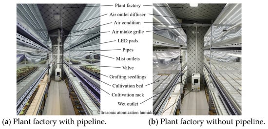
Figure 1. Test plant factory (26 °C, 60% RH).

2.2. Experimental Methods

Temperature and humidity sensors (RC-4HC, operating range −30 °C to +60 °C with ±0.5 °C accuracy; 0% to 100% RH with ±3% accuracy, Jiangsu Jingchuang Electric Co., Ltd., Xuzhou, China) were installed in the plant factory. These sensors were specifically employed to continuously monitor and record the dynamic environmental temperature and relative humidity within the controlled production facility. The spatial configuration of the integrated sensor network is illustrated in Figure 2. The pipeline humidification system is misted by an ultrasonic atomization humidifier (CR-09, 9 kg/h, 400 W, 430 × 430 × 290 mm, Shanghai Chiyi Automotive Supplies Co., Ltd., Shanghai, China). It can evenly generate mist droplets smaller than 5 μm, with an air velocity of 5 m/s. Driven by high-speed airflow, the droplets collide and thoroughly mix inside the pipeline to ensure uniform distribution before being delivered under pressure to the different cultivation shelves. With the ultrasonic humidifier operating at a constant power level, the pipeline humidification system was used to increase the humidity in the cultivation space. The water lost through atomization was replenished in time to keep the humidifier’s water tank at a constant volume of 5 L. These measures provided stable external humidification conditions and reduced the influence of the ultrasonic humidifier itself on humidity control. To systematically describe the spatial distribution of temperature and relative humidity, four cultivation shelves were used, with multiple sensors arranged to create a total of 12 measurement points. The data logger was set to record temperature and humidity every 20 s, and the collected data were exported every two days for further analysis and processing.

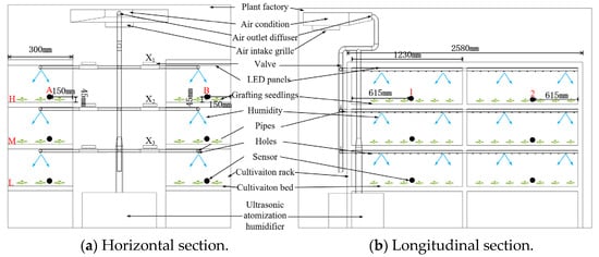
Figure 2. Location of sensors in the plant factory. Note: Arabic numerals 1-2 represent sensors for temperature and relative humidity distribution inside plant factories; capital letters H, M, and L represent three vertical heights, while capital letters A and B represent two horizontal distances.

2.3. Experimental Design

The quadratic regression orthogonal rotation combination design method was employed to investigate the influence of valve opening on the MRH and establish a relative humidity prediction model. Since seedling transpiration and respiration alone cannot raise the relative humidity in the cultivation space to the optimal level for wound healing—above 90%—and may even cause a continuous decrease in moisture content [32], the only way to increase the relative humidity is by adjusting the valves on the humidification pipeline to provide sufficient levels for the grafted seedlings. Consequently, the valve-opening degree of each layer can be approximated as the primary factor influencing the relative humidity of the cultivation shelf. Considering the longitudinal spatial distribution of the valves, the upper and lower control limits for those on the first, second, and third layers were uniformly defined as 0° and 90°, respectively. Therefore, the average zero point (Z_0j) for each factor was determined as 45° using the following formula:

$$Z_{0j}={\displaystyle \frac{Z_{1j}+Z_{2j}}{2}}$$

(1)

where Z_J represents the factor, and Z_1j and Z_2j denote the minimum and maximum values of the factor’s level change, respectively. The zero level Z_0j is calculated as half the sum of Z_1j and Z_2j.

The variation range (${\Delta }_j$) of the preparation factor level can be expressed by the following formula:

$${\Delta }_j={\displaystyle \frac{Z_{2j}-Z_{0j}}{\gamma }}$$

(2)

where ${\Delta }_j$ represents the variation interval, $\gamma$ is the star arm, and the test factor levels are set as $-\gamma$, $-1$, $0$, $1$, $\gamma$. The value of $\gamma$ can be calculated using the following formula:

$$\gamma =2^{\left({\displaystyle \frac{m-i}{4}}\right)}$$

(3)

where m is the number of factors, m = 3, and $i$ is the implementation index. For a fully implemented test, $i=0$, and the $\gamma$ value is 1.682. The calculated opening values ${∆}_j$ for the first, second, and third valves were approximately 26.75; these were rounded to 27 for practical application.

Test factor level values were selected based on the project team’s experience and pre-test data, following the quadratic regression orthogonal rotation combination design. The number of test points ($N_S$) for 3 factors at 5 levels was determined as follows:

$$N_S=m_c+m_r+m_o$$

(4)

where m_c test points are distributed on a sphere with a radius ${\rho }_c=\sqrt{m}$ in the normal variable space; m_r = 2m test points are distributed on a sphere with a radius ${\rho }_{\gamma }=\gamma$ in the space of normal variables; and m₀ test points are distributed on the spherical surface of radius ${\rho }_c=\gamma$ in the space of normal variables, specifically the zero horizontal points. When the test is fully implemented, $m_c=2^m=2^3=8$; m_r is the number of star points, $m_r=2\mathrm{m}=6$ and m₀ is the number of center points. To ensure a degree of orthogonality in the quadratic regression orthogonal rotation combination design, m₀ must satisfy the following requirement:

$${\displaystyle \frac{N_S\left(m{m}_c+2{\gamma }^4\right)}{\left(m+2\right){\left(m_c+2{\gamma }^2\right)}^2}}=1$$

(5)

Calculations determined the number of trials (N_S) to be 23, yielding a derived value of m₀ = 9. Based on the aforementioned formulas, the encoding table for the factor levels, including the first-, second-, and third-layer valve-opening degrees, was constructed, as shown in Table 1.

Table 1. Test factors and levels.

Test Number	X1/°	X2/°	X3/°	MRH/%
1	79.2	79.2	79.2	89.9
2	79.2	79.2	10.8	88.8
3	79.2	10.8	79.2	89.1
4	79.2	10.8	10.8	88.3
5	10.8	79.2	79.2	84.3
6	10.8	79.2	10.8	83.8
7	10.8	10.8	79.2	84.5
8	10.8	10.8	10.8	84.8
9	90.0	45.0	45.0	88.6
10	0.0	45.0	45.0	81.0
11	45.0	90.0	45.0	89.1
12	45.0	0.0	45.0	87.4
13	45.0	45.0	90.0	88.5
14	45.0	45.0	0.0	87.1
15	45.0	45.0	45.0	90.2
16	45.0	45.0	45.0	90.3
17	45.0	45.0	45.0	90.5
18	45.0	45.0	45.0	90.7
19	45.0	45.0	45.0	90.7
20	45.0	45.0	45.0	90.8
21	45.0	45.0	45.0	90.2
22	45.0	45.0	45.0	90.5
23	45.0	45.0	45.0	91.0

2.4. Test Procedure

The experiment was carried out in a controlled environment. There were a total of 23 valve combinations, with each tested three times. Before testing, RC-4HC temperature and humidity sensors were placed at multiple positions on each layer of the cultivation shelves to ensure full spatial coverage for environmental monitoring. The detailed experimental procedure is described below.

Step 1: Adjust the valves according to the preset parameters for each experimental group to regulate the required airflow.

Step 2: Monitor the temperature shown on the temperature control box. If the temperature inside the plant factory is below 25.5 °C, allow the system to stabilize until it reaches 25.5 °C. If it exceeds this temperature, activate the cooling system until the temperature stabilizes at this value. Once the ambient conditions are stable, record the cooling duration and corresponding humidity values before beginning the experiment.

Step 3: Continue monitoring the temperature on the controller until it drops to 24 °C. At this point, turn off the air conditioner using the temperature control box to end the cooling phase.

Step 4: Activate the humidification system remotely via Bluetooth control. When the relative humidity exceeds 60%, record both the humidification start time and the spatial humidity values at each measurement point.

Step 5: Use the dedicated mobile application to continuously track real-time relative humidity in the plant factory. When the RH reaches 90%, turn off the humidifier to prevent excessive humidity.

Step 6: Calculate the MRH of the experiment, starting from a humidity value greater than or equal to 90%, until it decreases again to 90%.

Step 7: Each experimental group followed this procedure three times to ensure data accuracy and reproducibility.

2.5. Machine Learning

Machine learning techniques have become increasingly pivotal in optimizing agricultural processes, particularly within controlled environments such as plant factories. Among these techniques, Random Forest, Transformer models, and XGBoost have demonstrated considerable potential in enhancing prediction accuracy and decision-making processes.

2.5.1. Random Forest

A Random Forest regression model was adopted to predict the temporal evolution of relative air humidity in the valve-controlled pipeline humidification system. As illustrated in Figure 3, the original dataset was first subjected to bootstrap sampling to generate multiple training subsets. A decision tree regressor was constructed for each of these by recursively partitioning the feature space, where a random subset of candidate variables was considered at each split. This randomization in both samples and features decorrelated the individual trees and reduced the risk of overfitting compared with a single decision tree.

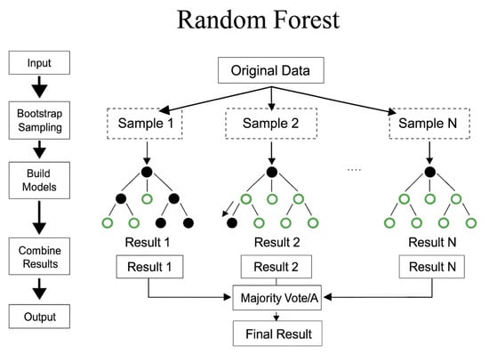
Figure 3. Random Forest framework.

After feature engineering, the dataset was divided into training (80% of the samples) and testing sets (20% of the samples), in chronological order and without shuffling in order to preserve the time dependence and emulate realistic forecasting conditions. The Random Forest ensemble consisted of 100 decision trees with a maximum depth of 10, a minimum of 5 samples required to split an internal node, and at least 2 samples in each terminal node. A fixed random seed was used to ensure result reproducibility. During prediction, each decision tree produced an individual humidity estimate for a given input, and the final output of the Random Forest model was obtained as the arithmetic mean of all tree predictions, corresponding to the “combine results” and “final result” steps shown in Figure 3. The overall predictive model [33] can be represented as follows:

$${\widehat{y}}_i={\displaystyle \frac{1}{M}}{\displaystyle \sum _{m=1}^M{f}_m}(x_i)$$

(6)

where ŷᵢ denotes the predicted humidity for the ith observation, xᵢ is the feature vector, f_m represents the prediction from the mth decision tree, and M is the total number of trees.

2.5.2. XGBoost

An extreme gradient boosting (XGBoost) regression model was employed to predict the temporal evolution of relative humidity in the plant factory. As illustrated schematically in Figure 4, XGBoost constructs an ensemble of regression trees in an additive manner, where each successive tree is trained to fit the residuals of the previous ones. The final prediction is obtained by summing the weighted outputs of all individual trees, which allows complex nonlinear relationships between the inputs and humidity to be captured while controlling model complexity through regularization and learning-rate scaling.

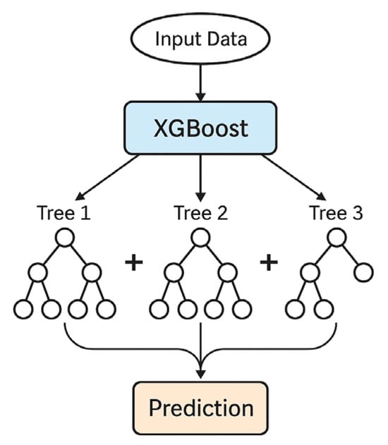
Figure 4. XGBoost schematic diagram.

The XGBoost model was implemented using the XGBRegressor algorithm. The ensemble consisted of 100 regression trees, with the maximum tree depth limited to 6 to prevent overfitting while maintaining sufficient expressive power. A learning rate of 0.05 was adopted so that trees were added gradually and the optimization process remained stable. To enhance generalization, row and column subsampling were applied, with 90% of the training samples used for each tree (subsample = 0.9) and 90% of the features randomly selected at each split. A fixed random seed was used to ensure reproducibility. The overall predictive model [25] can be expressed as follows:

$$i={\displaystyle \sum _{k=1}^K{f}_k}(x_i),\hspace{1em}{f}_k\in \mathcal{F}$$

(7)

where ŷᵢ denotes the predicted humidity for the ith sample, xᵢ is the feature vector, fₖ represents the kth regression tree, and K is the total number of trees.

2.5.3. Transformer

In this study, a Transformer-based deep learning model was employed to predict short-term humidity variations. Compared with tree-based models that rely on explicit feature construction, the Transformer architecture captures temporal dependencies and long-range correlations directly from the time series [34]. As illustrated in Figure 5, the model adopts an encoder–decoder structure composed of stacked multi-head self-attention layers and position-wise feed-forward networks.

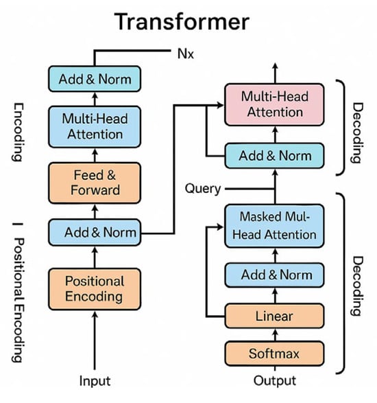
Figure 5. Transformer schematic diagram.

The input sequence X = [x₁, x₂, …, x_T] is first linearly projected into a latent feature space using an embedding layer:

$$Z=X{W}_e+b_e,\hspace{1em}Z\in {ℝ}^{T\times d_{\mathrm{model}}}$$

(8)

where X represents the input sequence, W_e represents the embedding weight matrix, b_e represents the embedding bias, Z represents the projected feature sequence, $Z\in {ℝ}^{T\times d_{\mathrm{model}}}$ represents the dimension of the output matrix, d model represents the model dimension of the Transformer model, and d_model denotes the embedding dimension.

Since the Transformer lacks inherent temporal awareness, sinusoidal positional encoding is added to each embedding to provide explicit time-step information. The enriched sequence is then passed into the encoder, where the multi-head self-attention mechanism evaluates its relative importance among different historical steps. The attention operation is defined as follows:

$$\mathit{Attention}(Q,K,V)=\mathit{softmax}\left({\displaystyle \frac{Q{K}^T}{\sqrt{d_k}}}\right)V$$

(9)

where Q, K, and V represent the query, key, and value matrices, respectively, and d_k is the key dimension. This mechanism enables the model to dynamically learn which historical humidity patterns most strongly influence future values. Multiple encoder layers further refine the contextual representation, and the final hidden state is fed into a regression head to generate next-step prediction:

$${\widehat{y}}_t=f_{\mathrm{Transformer}}(x_{t-L:t-1})$$

(10)

where ${\widehat{y}}_t$ indicates the predicted value of the model at time t, $f_{\mathrm{Transformer}}$ represents the function mapping relationship corresponding to the Transformer model, and $x_{t-L:t-1}$ represents the historical series data from time t − L to t − 1, with a length of L.

The model is optimized using the mean squared error loss function:

$$\mathcal{L}={\displaystyle \frac{1}{N}}{\displaystyle \sum _{i=1}^N{(y_i-{\widehat{y}}_i)}^2}$$

(11)

where $\mathcal{L}$ represents the loss value, N represents the number of samples, y_i represents the ground actual value of the i-th sample, and ${\widehat{y}}_i$ represents the model prediction of the i-th sample. The Adam optimizer with a learning rate of 1 × 10⁻³ was applied to accelerate convergence.

Prior to training, the humidity series was normalized using Min–Max scaling and divided into training and testing sets with an 80:20 ratio. The model was trained using a sliding-window dataset of fixed sequence length and early stopping, as well as adaptive learning-rate scheduling, was applied to prevent overfitting. During inference, the model performs recursive multi-step forecasting, where each newly predicted value is iteratively fed back into the input sequence to forecast humidity for the subsequent 30 min.

2.6. Evaluation Metrics

The RH in the plant factory is described as being uniform by Zhang et al. [35] and Chowdhury et al. [36]. In this paper, the evaluation criteria are the MRH and CV_RH.

$$\mathit{MRH}={\displaystyle \sum _{i=1}^{n}R{H}_i},n=12$$

(12)

$$C{V}_{RH}={\displaystyle \frac{\sqrt{{\displaystyle \sum _{i=1}^n\left(R{H}_i-R{H}_a\right)}}}{R{H}_a}}$$

(13)

where i represents the column number of the measurement point, n denotes the total number of measurement points, CV_RH is the coefficient of variation in relative humidity, ${RH}_i$ is the measured value of relative humidity, and ${RH}_a$ is the average relative humidity.

To evaluate and compare the performance of the predictive models, several statistical metrics were employed: the coefficient of determination (R²), mean absolute error (MAE), mean squared error (MSE), and root mean squared error (RMSE). These indicators provide quantitative insights into the effectiveness of the developed models. A higher R² value indicates better model performance, as it reflects a stronger correlation between the predicted and observed data [37]. Conversely, lower MAE, MSE, and RMSE values indicate superior model accuracy, as these are error-based metrics. Values closer to zero represent a more precise prediction performance.

The evaluation metrics are calculated as follows:

$$R^2=1-{\displaystyle \frac{{\displaystyle \sum _i{(y_i-{\widehat{y}}_i)}^2}}{{\displaystyle \sum _i{(y_i-\overline{y})}^2}}}$$

(14)

$$MAE={\displaystyle \frac{{\displaystyle \sum \left(\left|y_i-{\widehat{y}}_i\right|\right)}}{n}}$$

(15)

$$MSE={\displaystyle \frac{{\displaystyle \sum {\left(y_i-{\widehat{y}}_i\right)}^2}}{n}}$$

(16)

$$RMSE=\sqrt{{\displaystyle \frac{{\displaystyle \sum {\left(y_i-{\widehat{y}}_i\right)}^2}}{n}}}$$

(17)

where y_i is the true value of the sample, $\widehat{\mathrm{y}}$_i is the predicted value of the sample, and n is the number of samples.

3. Results

3.1. Regression Modeling of Relative Humidity in Plant Factories

The experimental factors—including the first (X₁), second (X₂) and third (X₃) valve openings—were analyzed using Design-expert 13.0 software, with the experimental design and corresponding results shown in Table 1. The data were analyzed for significance using ANOVA (Analysis of Variance), the results of which are shown in Table 2. According to these results, the expression of the quadsratic regression model between the relative humidity and X₁, X₂ and X₃ was obtained as follows:

$$\begin{array}{c}{\overline{X}}_{RH}=0.129518X_1+0.030456X_2+0.042951X_3\\ +0.000155X_1{X}_2+0.000098X_1{X}_3+0.000078X_2{X}_3\\ -0.000997X_1^2-0.000401X_2^2-0.000481X_3^2+84.51747\end{array}$$

(18)

Table 2. ANOVA and error statistics.

Source	Sum of Squares	df	Mean Square	F-Value	p-Value
Model	147.72	9	16.41	130.68	<0.0001	significant
A	72.41	1	72.41	576.53	<0.0001	significant
B	0.6505	1	0.6505	5.18	0.0461	significant
C	1.58	1	1.58	12.55	0.0053	significant
AB	0.7844	1	0.7844	6.25	0.0315	significant
AC	0.3178	1	0.3178	2.53	0.1428	not significant
BC	0.199	1	0.199	1.58	0.2367	not significant
A2	58.75	1	58.75	467.76	<0.0001	significant
B2	9.49	1	9.49	75.57	<0.0001	significant
C2	13.7	1	13.7	109.08	<0.0001	significant
Residual	1.26	10	0.1256
Lack of Fit	0.886	5	0.1772	2.39	0.18	not significant
Pure Error	0.37	5	0.074
Cor Total	148.97	19

As shown in Table 2 and Table 3, the p-value of the model is less than 0.0001, and the R² value is 0.9907. These results indicate that the model can accurately describe the relationship between the MRH and the valve openings of the first, second, and third layers. The F-test of the model showed that the variance probability of the model’s misfit was not significant, indicating a good model fit, and the MRH variation coefficient was nonlinear with X₁, X₂ and X₃. The influence factor values of the three factors were 576.53 for X₁, 5.18 for X₂, and 12.55 for the valve opening of the X₃, and their relative values were 72.41%, 0.65% and 1.58%, respectively. According to the principle that the larger the F value, the more significant the three factors’ influence on the uniformity coefficient of the cultivation frame, their significance on the MRH is as follows: X₁ > X₃ > X₂. The airflow near X₁ is stronger due to its closer proximity to the main air outlet, resulting in higher humidity transport efficiency. X₃ receives moderate airflow due to partial obstruction and increased diffusion distance, while X₂ is located in a region with weaker airflow circulation, leading to reduced humidity transfer.

Table 3. Model credibility analysis.

Reference	Model
R2	0.9907
Adjusted R2	0.9843
Predicted R2	0.9527
C.V.%	0.3929

3.2. Regression Model Analysis

Figure 6 shows the fitting residual plot of MRH in the cultivation shelf, which indicates that the lower the regression fit, the larger its residual value and the farther the points in the plot are from the diagonal line. As can be seen in Figure 6a, most of the points are distributed on both sides of the straight line and close to it, indicating that the fit is good and the test results are reliable. Figure 6b shows the correspondence between the actual test values and the predicted values of the MRH of the cultivation frame. The slope of the diagonal line in the graph is 1, which indicates that the MRH experimental values in the cultivation shelf, the predicted values, and the points are distributed on both sides of the diagonal line. In turn, this suggests that the model has a better fit and higher prediction accuracy.

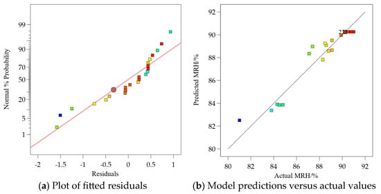
Figure 6. Modeling of MRH in cultivated racks.

3.3. One-Way Test Result Analysis

Figure 7 illustrates the effect of valve openings on the MRH for each layer. As shown in Figure 7a, when X₂ and X₃ were both set at 45°, the relationship between MRH and X₁ was expressed as MRH(X₁) = −0.01X₁² + 1.2X₁ + 55. According to this equation and Figure 7a, MRH reached its maximum value when X₁ was 60°. From 0° to 60°, MRH increased with the increase in X₁, which is consistent with the findings of Santiago Bonachela et al. [38]. When the valve opening increased from 60° to 90°, MRH slightly decreased. This could be attributed to the fact that as relative humidity increased, the water absorption capacity of the substrate and plant transpiration reached their upper limits. Consequently, excess moisture could not be absorbed, leading to air saturation. When humid air continued to enter, some moisture condensed due to oversaturation, resulting in a slight decrease in MRH.

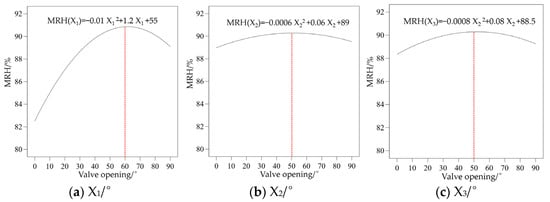
Figure 7. Variation in MRH of cultivation shelves with valve openings (The red dashed line represents the valve opening corresponding to the point where MRH reaches its peak).

As shown in Figure 7b, when X₁ and X₃ were both 45°, the relationship between MRH and X₂ was MRH(X₂) = −0.0006X₂² + 0.06X₂ + 89. According to this relationship and Figure 7b, MRH reached its maximum when X₂ was 5im0°. As X₂ gradually increased, MRH first rose and then declined, which may be due to the environment approaching saturation, where high humidity inhibits further water evaporation.

As can be seen in Figure 7c, when X₁ and X₂ were both 45°, the relationship between MRH and X₃ was MRH(X₃) = −0.0008X₃² + 0.08X₃ + 88.5. With the increase in X₃, MRH showed a similar trend of first rising and then decreasing, reaching its maximum value when X₃ was 50°.

Based on the above analysis, when X₁, X₂, and X₃ are set to 60°, 50°, and 50°, respectively, MRH reaches its maximum value.

3.4. Independent Variable Interactions with the MRH

Response surface analysis was used to examine the relationships among multiple influencing factors and their interactions, as well as their effects on the response variable. This method helps to reveal the complex interdependence between variables, providing a clearer understanding of how they jointly affect the outcome. Based on the regression model (Equation (8)) established in the previous section, response surface plots were generated, as shown in Figure 8. To evaluate the effect of the interaction between any two valve openings on the MRH, one variable (X₁, X₂, or X₃) was held constant in each analysis.

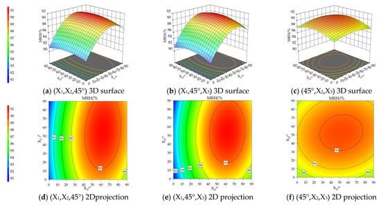
Figure 8. The interaction influence of MRH.

The degree of variation in the response surface reflects the strength of the interaction between two factors. Greater fluctuations indicate stronger interaction effects, while flatter surfaces suggest weaker interactions. As shown in Figure 8a,d, when X₃ was fixed at 45°, MRH increased as both X₁ and X₂ rose to 75°, but began to decline once they exceeded 80°. Notably, MRH already exceeded 90% when both X₁ and X₂ were at 45°, satisfying the high-humidity requirements for grafted seedlings. Conversely, Figure 8b,f show that when X₂ was fixed at 45°, both X₁ and X₃ exhibited a similar increasing-then-decreasing trend. MRH reached the 90% threshold when X₁ and X₃ were at 45°, but decreased once the valve openings exceeded 80°.

By integrating the results from Figure 8a,b,d,e, we determined that the optimal valve opening for X₁ is 60°, as this setting places MRH near the central region of the response surface. Similarly, Figure 8a–c, and f indicate that X₂ at 50° produces the most balanced MRH response, while Figure 8b,c,e,f suggest that X₃ at 50° provides the most appropriate setting. Overall, the analysis shows that setting X₁, X₂, and X₃ to 60°, 50°, and 50°, respectively, keeps MRH above 90% and maximizes its overall value.

3.5. Regression Model Validation

To verify the accuracy and general applicability of the model, validation experiments were conducted. The valve openings for the first, second, and third layers were set to 60°, 50°, and 50°, respectively. Four parallel tests were performed, and the humidity across 12 measurement points ranged from 90.2% to 91.3%. As shown in Table 4, the experimental RH values were compared with the theoretical ones predicted by the model. The theoretical RH was 90.51%, while the experimental values were 90.98%, 91.14%, and 91.23%. The maximum relative error between the theoretical and experimental results was 0.62%, the minimum was 0.03%, and the average was 0.67%. Additionally, validation tests were conducted for the ten non-optimal experimental groups. The largest error occurred in the combination 10.8°, 10.8°, 10.8°, with a relative error of 5.10%, while the smallest error was observed in the combination 0°, 45°, 45°, with a relative error of 0.91%. For most experimental groups, the relative error was below 5%, indicating high reliability. The experimental results were in close agreement with the model predictions, indicating that the regression model can reliably predict the relative humidity on the cultivation shelf under different valve-opening conditions.

Table 4. Validation results of the regression model’s theoretical predicted MRH values, experimental measured MRH values, and relative errors under different combinations of valve opening parameters.

Test Number	X1/°	X2/°	X3/°	Theoretical Value/%	Experimental Value/%	Relative Error/%
1	60	50	50	90.51	91.12	0.67%
2	79.2	79.2	10.8	88.58	90.89	2.61%
3	10.8	79.2	10.8	83.37	81.83	1.85%
4	90	45	45	89.09	93.46	4.91%
5	0	45	45	82.50	83.25	0.91%
6	79.2	79.2	79.2	89.96	91.79	2.03%
7	79.2	10.8	79.2	88.66	84.32	4.90%
8	10.8	10.8	79.2	83.85	82.17	2.00%
9	10.8	10.8	10.8	83.86	79.58	5.10%

3.6. Comparative Analysis

The control group consisted of melon seedlings placed in a plant factory without pipeline installation. Each experimental cycle included a cooling phase, during which the temperature decreased from 26.5 °C to 25 °C, and a humidification phase, where the relative humidity increased from a dehumidified state to 90%. At the end of each experiment, the time was recorded to match the corresponding humidity values at each cultivation shelf layer. Both the control and optimization groups used ultrasonic atomization humidifiers as moisture sources. The main difference was that the optimization group incorporated valves to regulate moisture supply for each layer, applying the optimal valve-opening settings derived from the quadratic regression orthogonal rotation combination design to achieve precise humidity control. A comparison between the two groups is shown in Figure 9.

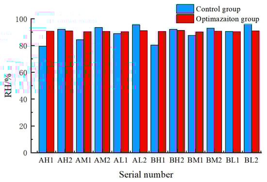
Figure 9. Relative humidity between optimization and control groups.

To ensure proper melon seedling healing, the humidity within the cultivation trays needed to exceed 90%. In the control group, five locations failed to meet this requirement: AH1, AM1, AL1, BH1, and BM1. Among them, AH1 and BH1 were about 10% below the standard, while the remaining three points were 1.1% to 5.7% lower than required. In contrast, the optimization group consistently maintained humidity levels above 90%, with uniform distribution across all layers. The maximum humidity recorded was 91.3%, the minimum was 90.2%, and the average was 90.7%, indicating excellent uniformity among the cultivation shelves. Compared with conventional PID-based humidity control [39], which adjusts actuator outputs through real-time feedback and requires careful parameter tuning, the proposed method adopts a fundamentally different strategy. PID controllers are simple and widely used, but their performance often degrades under nonlinear, delayed, or multi-layer coupled environments. In contrast, this study models the nonlinear relationship between valve opening and MRH using a quadratic orthogonal rotation regression design, enabling spatial humidity uniformity maximization.

Overall, compared with the conventional humidification method, the valve-controlled pipeline humidification system significantly improved humidity performance. The compliance rate of relative humidity increased from 58.3% to 100%, the average relative humidity rose from 89.4% to 90.7%, and the humidity variation decreased from 6.1% to 0.3%. This demonstrates that the valve-controlled system greatly enhances humidity uniformity across all cultivation layers. However, as seedlings grow, further studies will be needed to assess how plant respiration and transpiration influence humidity. Moreover, for other crops, such as lettuce [20] and dendrobium [40], valve openings may need to be adjusted according to different growth stages. It is also worth noting that the healing phase for melon grafted seedlings lasts only about one week before transplantation.

3.7. Effects of Valve Openings on the Dynamic Variation of Relative Humidity During the Humidification Process

To further analyze the influence of valve openings on the humidification process, the real-time variation in relative humidity under different valve configurations was recorded and visualized. Figure 10 presents the dynamic changes observed during humidification. Throughout the experiment, sensors continuously monitored and recorded humidity variation in real time, capturing the complete transition from the pre-cooling stage to the post-cooling humidification phase.

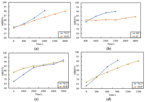
Figure 10. The relative humidity change rule in the humidification process. (a) Variation with X₁ at fixed X₂ = 79.2°, X₃ = 10.8°; (b) Variation with X₁ at fixed X₂ = 45.0°, X₃ = 45.0°; (c) Variation with X₂ at fixed X₁ = 79.2°, X₃ = 79.2°; (d) Variation with X₃ at fixed X₁ = 10.8°, X₂ = 10.8°.

As shown in Figure 10a, when the first-layer valve openings were set at different angles, the time required to reach 90% relative humidity—RH—varied significantly. For example, a valve opening of 10.8° required about 4000 s, whereas an opening of 79.2° achieved the same RH in only 2400 s, saving approximately 1600 s. Under conditions with minimal humidity loss, the valve-opening degree directly determines the moisture supplied to the cultivation shelves. A positive correlation exists between the valve opening and the rate of moisture addition per unit area, with larger openings generally providing faster humidification. This explains why the 79.2° valve reached the target RH sooner. These findings are consistent with those of S.A. El-Agouz et al. [41], who reported that increasing the air intake per unit area markedly enhances humidification efficiency.

Figure 10b presents the results when the second- and third-layer valves were both fixed at 45°, while the first-layer valve was either fully open, 90°, or fully closed, 0°. When the first-layer valve was open, RH increased from 77% to 90% within 3200 s. However, when the valve was closed, RH remained almost unchanged until 3200 s and reached only 85% after 4800 s. This demonstrates the good airtightness of the valve system. After 3200 s, the indoor environment likely became supersaturated, causing a slight RH increase due to moisture diffusion from other layers.

Figure 10c compares the humidification performance of the first-layer valve at 10.8° and 79.2°, with the second- and third-layer valves fixed at 45°. Both openings eventually achieved the target RH, with similar humidification times of around 5000 s. Notably, the initial RH for the 10.8° valve, approximately 77%, was higher than for the 79.2° valve, around 67%, indicating that the larger 79.2° opening achieved faster humidification under the same conditions. Guo et al. [42] also found that increasing the number of spray nozzles improves humidification performance, supporting the observation that a larger valve-opening angle enhances overall efficiency.

Figure 10d shows the humidification time required for the third-layer valve at openings of 10.8° and 79.2° to raise RH from 71% to 90%. The 10.8° opening took about 4000 s, while the 79.2° opening required only 2400 s. This marks a difference of 1600 s, again confirming the positive correlation between the valve opening and humidification rate.

3.8. Machine Learning in Humidity Prediction

To evaluate the performance of different prediction methods for humidity regulation in the grafted seedling plant factory, machine learning models were used to forecast short-term changes in relative humidity. These models can capture complex nonlinear relationships among environmental factors, providing a reliable reference for achieving precise humidity control in grafting environments.

After training the three machine learning models, their relative humidity prediction performance was evaluated and compared. The analysis focused on how accurately each model could capture short-term humidity variations within the 0–6-h forecasting window. To ensure a comprehensive assessment, several statistical indicators were used, including R², MAE, MSE, and RMSE. These metrics provide an overall understanding of each model’s predictive accuracy and stability under different time intervals.

A total of 1500 samples of relative humidity data collected from the plant factory were used to predict RH over the next 6 h. During model training, the dataset was divided into three subsets: a training, validation, and testing set. Figure 11 shows the humidity prediction results obtained using different models. The R² values for the Random Forest, XGBoost, and Transformer models were 0.9543, 0.9505, and 0.8789, respectively, corresponding to a time interval of 3 min.

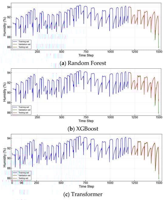
Figure 11. Performance of three machine models.

3.9. Performance of Three Models in Relative Humidity Prediction

Figure 12 shows a comparative analysis of the three predictive models over the 0–6-h forecasting period. When evaluating model performance, a higher R² value closer to 1 and lower MAE, MSE, and RMSE values closer to 0 indicate better prediction accuracy. Therefore, models with results approaching these ideal values are considered to perform more effectively overall.

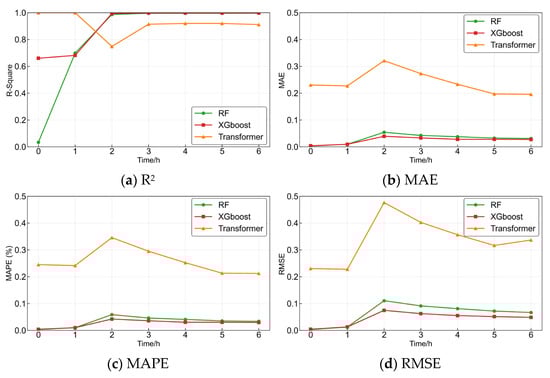
Figure 12. Performance of three machine models over 0–6 h.

The maximum R² values of the Random Forest, XGBoost, and Transformer models were 0.9965, 0.9982, and 0.9202, respectively, while the minimum values were 0.0337, 0.6602, and 0.3180. During the 0–2-h period, all three models showed relatively low R² values. As the forecasting period extended to 2–6 h, the R² values of the Random Forest and XGBoost models increased to above 0.98, while that of the Transformer exceeded 0.91 between 3 and 6 h.

The maximum MAE values of the three models were 0.0542, 0.0393, and 0.3210, with corresponding minimum values of 0.0031, 0.0039, and 0.1958. Throughout the 0–6-h prediction period, the MAE values of Random Forest and XGBoost remained consistently lower than those of the Transformer, indicating higher accuracy. Similarly, the maximum MAPE values were 0.0587, 0.0432, and 0.3457, and the minimum values were 0.0033, 0.0041, and 0.2123 for the three models, respectively. Across all time intervals, Random Forest and XGBoost achieved smaller MAPE values than the Transformer, further confirming their superior predictive performance.

In addition, the maximum RMSE values for the three models were 0.1106, 0.0747, and 0.4764, while the minimum values were 0.0033, 0.0043, and 0.2277. Consistent with the MAE and MAPE trends, the RMSE values of Random Forest and XGBoost were significantly smaller than those of the Transformer throughout the 0–6-h period, demonstrating their higher prediction stability and precision.

4. Discussion

Previous studies by Lee et al. [30], Pérez-Alfocea et al. [31], and Kim et al. [32] found that maintaining a high-humidity environment accelerates grafted seedling healing. Based on this principle, this study designed an independent pipeline humidification testing platform and used a quadratic regression orthogonal rotational combination design to analyze the optimal valve-opening combination. The proposed method provided excellent MRH and significantly reduced humidity unevenness compared to the control group.

The quadratic regression orthogonal rotation design successfully predicted the dynamic relative humidity in multi-layer pipe humidification systems, showing high predictive accuracy with an R² value of 0.99 and strong agreement between observed and predicted results. This method has been widely recognized for investigating complex multi-factor interactions and optimizing parameters in agricultural and environmental engineering [19,22,43]. A similar predictive performance was reported by Chen et al. [44], who achieved an R² of 0.95 for fog-based humidity control in lettuce plant factories, as well as by Gao et al. [45], who obtained an R² of 0.97 for CFD-calibrated humidity uniformity in vertical farms. The low average relative error of 0.67% observed in this study is consistent with the 0.90% reported by Choi et al. [46] for a dehumidification-integrated heat pump system, confirming the reliability of second-order polynomial models in small-scale plant factory environments. You et al. [47] studied the relationships between humidity, temperature, wind speed, and humidity ratio using regression equations and proposed solutions to reduce condensation on building surfaces. This mechanism is similar to the principle of the model used in this study, which aims to reduce the risks associated with excessive humidity.

The ANOVA results showed that the first-layer valve opening accounted for 72.57% of the humidity variance, which was much higher than that of the third and second layers, at 1.45% and 0.64%, respectively. This pattern is consistent with the findings of Kozai et al. [1], who reported that buoyancy-driven air movement causes upper humidifiers to dominate overall chamber humidity. The low contribution of the second layer suggests that air circulation in the 2.26 m chamber minimized the influence of mid-level injection, which aligns with the results of Kang et al. [48] in multi-tier Chinese cabbage systems. The response surface analysis showed that humidity increased with valve opening and reached its maximum at 60°, 50°, and 50° for the first, second, and third valves, respectively, before decreasing. This convex relationship reflects the saturation point of the cultivation substrate and plant transpiration, which supports Bonachela’s [38] hypothesis on saturation and condensation in hydroponic cucumber systems.

The temperature reduction followed by humidification strategy used in the experiment was essential in preventing fogging and condensation inside the pipelines, which could affect sensor accuracy and seedling health [44]. This approach ensured reliable data collection during the critical humidification stage. Increasing the valve openings from 10.8° to 79.2° reduced the humidification time by about 1600 s, highlighting the advantage of adjusting airflow instead of maintaining a fixed rate. Similar results have been observed in other studies [32,34], where variable-speed fans and optimized perforated tubes improved humidity recovery speed and shortened humidification cycles. These results support the use of dynamic valve control to improve humidification efficiency, reduce energy consumption, and lower latent heat loads, which are key factors for energy-efficient plant factory operation.

Maintaining high MRH is also essential to prevent localized pathogen outbreaks, especially in grafting areas that are prone to Botrytis cinerea infection. Although the second-order model assumes a symmetrical response, excessive valve openings greater than 85° may cause turbulent airflow and condensation, reducing performance. Similar findings were reported by Gillingham et al. [49], who found that excessive fog duty cycles caused condensation that negatively affected seedlings in plant factories. Higher humidity promotes plant growth by allowing stomata to remain open, which enhances photosynthesis and reduces water loss. Chia and Lim [50] showed that the optimal relative humidity for plant growth ranges from 83% to 87%, which is close to the target value in this study. In the pipeline humidification test platform developed here, the MRH during experiments remained around 90%; once RH reached this level, the humidifier was immediately turned off to avoid condensation.

Reducing the temperature before humidification also helped prevent fogging and condensation in the pipelines, ensuring accurate sensor readings and maintaining healthy seedlings. Increasing valve openings from 10.8° to 79.2° shortened the humidification process by about 1600 s, showing flow adjustment’s advantage over fixed-speed systems. Similar improvements were reported in previous studies, such as faster humidity recovery using variable-speed fans [29] and shorter cycles achieved with perforated tube optimization. These findings highlight the importance of dynamic valve control to lower energy use and maintain stable humidity levels in plant factories.

Machine learning techniques are increasingly being used for humidity prediction in plant factories due to their strong ability to model nonlinear patterns. Table 5 shows the prediction performance of different machine learning methods. Rezaei Melal [24] and Wei et al. [25] compared multiple machine learning models to identify the most suitable approaches for humidity prediction. Rezaei Melal et al. [24] evaluated seven machine learning algorithms, ultimately selecting DT, RF, KNN, and XGBoost for humidity forecasting. In contrast, Wei et al. [25] compared BPPSO, LSSVM, and RBF models, determining that LSSVM as the optimal model for temperature and humidity prediction. Qin et al. [26] employed an optimized XGBoost model to predict air temperature, air pressure, and relative humidity. Their humidity prediction performance achieved R² = 0.95, RMSE = 0.32, MAE = 0.16, and MAPE = 0.28%. In the present study, the XGBoost model achieved an R² of 0.9517 for humidity prediction, and its RMSE, MAE, and MAPE were all below 0.2, indicating excellent short-term predictive capability. Kişmiroğlu and Isik [32] achieved notable progress in long-term forecasting using deep learning models. Their attention-based LSTM demonstrated strong long-horizon prediction performance; however, its short-term accuracy was relatively limited, with an MAE of 2.27. In this study, the attention-based deep learning model achieved a significantly lower MAE of 0.32. Finally, RF, XGBoost, and a Transformer model were employed for 6-h humidity forecasting. Their respective R² values were 0.9559, 0.9517, and 0.8789, demonstrating that RF exhibited the best performance for 6-h predictions.

Table 5. Prediction performance of different machine learning models.

Model Architecture	Prediction Performance	Prediction Object	Prediction Period	Reference
Transformer–LSTM Deep and Sarimax	Long term: MAE: 2.27, MSE: 6.63 Short term: MAE: 2.99, MSE: 14.92	Temperature	10 years and 5 months	Kişmiroğlu and Isik [32]
XGBoost	R2, RMSE, MAE, and MAPE of temperature were 0.88, 1.59, 0.79, 3.56%, RH were 0.95, 0.32, 0.16, 0.28%	Temperature and RH	5 months	Qin et al. [26]
MR, PR, DT, KNN, SVR, RF, XGBoost	R2, RMSE, MAE, and MAPE of temperature were 0.965, 0.001, 0.014, 3.20%	RH	4 months less	Rezaei Melal et al. [24]
BPPSO, LSSVM and RBF	R2, RMSE, MAE, and MAPE of temperature was 0.923, 0.867, 0.574, 1.94%, RH were 0.952, 3.97, 2.747, 3.38%	Temperature and RH	44 days	Wei et al. [25]
MLP-NN	The maximum errors of the modeled temperature and RH are 0.877 K and 2.838%, R2 both are 0.999.	Temperature and RH	62 days	Petrakis et al. [51]
RNN-BP	RMSE of temperature is 0.751, RH is 0.781, R2 is both above 0.9	Temperature and RH	A week	Hongkang et al. [52]

Another important limitation involves the model’s generalizability. Transpiration rates vary considerably among species and developmental stages. For example, tomato scions transpire approximately 20% more than melon seedlings under comparable environmental conditions [53], indicating that identical valve settings may not be suitable for all crops or growth stages. Future work may improve adaptability by introducing crop- or stage-specific parameters into the regression framework. Choi et al. [46] showed that incorporating such physiological modifiers enables broader applicability across solanaceous and cucurbit crops. Addressing these limitations would enhance the model’s versatility and support more reliable humidity management in diverse production scenarios.

Although this study has certain limitations—such as its lack of inclusion of real-time transpiration feedback, its testing of only on grafted seedlings, and its yet-to-be-validated large-scale applications—the proposed method has good adaptability. The framework can be customized for different climates, extended to vertical farms, and applied to other high-value crops beyond grafted seedlings. Overall, this study provides a reliable technical foundation for energy-efficient and precise humidity control in controlled-environment agriculture, which can improve grafting success, crop quality, and modern plant factory sustainability.

5. Conclusions

In this study, a valve-controlled pipeline humidification system was developed for multi-layer grafted seedling plant factories. A combination of quadratic regression modeling and machine learning-based humidity prediction was used to achieve precise humidity regulation. Based on the experimental and modeling results, the following conclusions can be drawn:

(1)

A quadratic regression model describing the relationship between valve opening and MRH was established using a quadratic rotation orthogonal combination design, achieving an R² of 0.9907. The humidification device improved layer-to-layer humidity uniformity from 6.1% to 0.3%, and repeated validations showed an average relative error of 0.67% under the optimal valve combination of 60°, 50°, and 50°.

(2)

Among the three prediction models evaluated, the RF model demonstrated the highest short-term humidity prediction accuracy. The proposed approach supports stable high-humidity conditions required for graft healing. Future work will focus on integrating the system into a closed-loop feedback control framework for real-time humidifier power and valve opening adjustment, enabling long-term robustness and scalable deployment.

References

- Kozai, T.; Japan, P.F.A. Towards sustainable plant factories with artificial lighting (PFALs) for achieving SDGs. Int. J. Agric. Biol. Eng. 2019, 12, 28–37. [Google Scholar] [CrossRef]
- Carotti, L.; Graamans, L.; Puksic, F.; Butturini, M.; Meinen, E.; Heuvelink, E.; Stanghellini, C. Plant Factories Are Heating Up: Hunting for the Best Combination of Light Intensity, Air Temperature and Root-Zone Temperature in Lettuce Production. Front. Plant Sci. 2021, 11, 592171. [Google Scholar] [CrossRef]
- Al-Kodmany, K. The Vertical Farm: A Review of Developments and Implications for the Vertical City. Buildings 2018, 8, 24. [Google Scholar] [CrossRef]
- Takagaki, M.; Hara, H.; Kozai, T. Micro- and mini-PFALs for improving the quality of life in urban areas. In Plant Factory; Elsevier: Amsterdam, The Netherlands, 2020; pp. 117–128. [Google Scholar]
- Cammarisano, L.; Körner, O. Response of Cyanic and Acyanic Lettuce Cultivars to an Increased Proportion of Blue Light. Biology 2022, 11, 959. [Google Scholar] [CrossRef] [PubMed]
- Chen, X.; Hou, T.; Liu, S.; Guo, Y.; Hu, J.; Xu, G.; Ma, G.; Liu, W. Design of a Micro-Plant Factory Using a Validated CFD Model. Agriculture 2024, 14, 2227. [Google Scholar] [CrossRef]
- Shamshiri, R.R.; Kalāntarī, F.; Ting, K.C.; Thorp, K.R.; Hameed, I.A.; Weltzien, C.; Ahmad, D.; Shad, Z.M. Advances in greenhouse automation and controlled environment agriculture: A transition to plant factories and urban farming. Int. J. Agr. Biol. Eng. 2018, 11, 1–22. [Google Scholar] [CrossRef]
- Tong, Y.; Oh, M.; Fang, W. Editorial: Advanced technologies for energy saving, plant quality control and mechanization development in plant factory. Front. Plant Sci. 2023, 14, 1193158. [Google Scholar] [CrossRef]
- Bhattarai, K.; Ogden, A.B.; Pandey, S.; Sandoya, G.V.; Shi, A.; Nankar, A.N.; Jayakodi, M.; Huo, H.; Jiang, T.; Tripodi, P.; et al. Improvement of crop production in controlled environment agriculture through breeding. Front. Plant Sci. 2025, 15, 1524601. [Google Scholar] [CrossRef]
- Kyriacou, M.C.; Colla, G.; Rouphael, Y. Grafting as a Sustainable Means for Securing Yield Stability and Quality in Vegetable Crops. Agronomy 2020, 10, 1945. [Google Scholar] [CrossRef]
- Haibo, Y.; Lei, Z.; Haiye, Y.; Yucheng, L.; Chunhui, L.; Yuanyuan, S. Sustainable Development Optimization of a Plant Factory for Reducing Tip Burn Disease. Sustainability 2023, 15, 5607. [Google Scholar] [CrossRef]
- Tirupathamma, T.L.; Ramana, C.V.; Naidu, L.N.; Sasikala, K. Vegetable Grafting: A Multiple Crop Improvement Methodology. Curr. J. Appl. Sci. Technol. 2019, 33, 1–10. [Google Scholar] [CrossRef]
- Wang, L.; Zhu, Z. Research on Temperature and Humidity Decoupling Control of Constant Temperature and Humidity Test Chamber. IOP Conf. Ser. Mater. Sci. Eng. 2020, 711, 12104. [Google Scholar] [CrossRef]
- Wei, J.; Xu, L.; Shi, Y.; Cheng, T.; Tan, W.; Zhao, Y.; Li, C.; Yang, X.; Ouyang, L.; Wei, M.; et al. Transcriptome profile analysis of Indian mustard (Brassica juncea L.) during seed germination reveals the drought stress-induced genes associated with energy, hormone, and phenylpropanoid pathways. Plant Physiol. Bioch. 2023, 200, 107750. [Google Scholar] [CrossRef]
- Saberian, A.; Sajadiye, S.M. Assessing the variable performance of fan-and-pad cooling in a subtropical desert greenhouse. Appl. Therm. Eng. 2020, 179, 115672. [Google Scholar] [CrossRef]
- Yang, S.; Yu, J.; Gao, Z.; Zhao, A. Energy-saving optimization of air-conditioning water system based on data-driven and improved parallel artificial immune system algorithm. Energy Convers. Manag. 2023, 283, 116902. [Google Scholar] [CrossRef]
- Wen, B.; Li, R.; Zhao, X.; Ren, S.; Chang, Y.; Zhang, K.; Wang, S.; Guo, G.; Zhu, X. A Quadratic Regression Model to Quantify Plantation Soil Factors That Affect Tea Quality. Agriculture 2021, 11, 1225. [Google Scholar] [CrossRef]
- Jung, D.H.; Lee, J. Establishing a Quadratic Regression Model of the Growth Characteristics and Isoorientin Contents of Wheatgrass Seedlings in Response to Different Temperature Conditions. Hortic. Sci. Technol. 2025, 43, 61–69. [Google Scholar] [CrossRef]
- Ghanbarzadeh Lak, M.; Sabour, M.R.; Amiri, A.; Rabbani, O. Application of quadratic regression model for Fenton treatment of municipal landfill leachate. Waste Manag. 2012, 32, 1895–1902. [Google Scholar] [CrossRef]
- Hosoda, Y.; Tada, T.; Goto, H. Lettuce Fresh Weight Prediction in a Plant Factory Using Plant Growth Models. Ieee Access 2024, 12, 97226–97234. [Google Scholar] [CrossRef]
- Wang, Y.; Liu, J.H.; Luo, Y.Z.; Zhou, X.X.; Ou, Y.Z.; Qi, H.J.; Yuan, Y. Numerical Analysis of Pneumatic Conveying Performance of Expanded Pellet Feed Based on CFD-DEM Coupling. Trans. Chin. Soc. Agric. Mach. 2025, 56, 180–189, 199. [Google Scholar]
- Rong, G.; Ning, Y.; Cao, X.; Su, Y.; Li, J.; Li, L.; Liu, L.; Zhou, D. Evaluation of optimal straw incorporation characteristics based on quadratic orthogonal rotation combination design. J. Agric. Sci. 2018, 156, 367–377. [Google Scholar] [CrossRef]
- Wang, H.; Fan, X.; Huang, M. Shearer parameter optimization and low energy consumption mining based on 3D point cloud characterization of coal wall. Energy Sci. Eng. 2024, 12, 736–754. [Google Scholar] [CrossRef]
- Rezaei Melal, S.; Aminian, M.; Shekarian, S.M. A machine learning method based on stacking heterogeneous ensemble learning for prediction of indoor humidity of greenhouse. J. Agric. Food Res. 2024, 16, 101107. [Google Scholar] [CrossRef]
- Wei, X.; Luo, Y.; Zhou, X.; Zhao, J.; Lu, H.; Li, J.; Zheng, J.; Li, B. Temperature and relative humidity prediction in South China greenhouse based on machine learning. Sci. Rep. 2025, 15, 24855. [Google Scholar] [CrossRef] [PubMed]
- Qin, Y.; Zhang, Y.; Duan, S.; Cao, Y.; Jia, X.; Chen, Q. Prediction and influencing factors analysis of stored grain temperature and intergranular relative humidity. Food Bioprod. Process 2025, 153, 67–76. [Google Scholar] [CrossRef]
- Qadeer, K.; Ahmad, A.; Qyyum, M.A.; Nizami, A.; Lee, M. Developing machine learning models for relative humidity prediction in air-based energy systems and environmental management applications. J. Environ. Manag. 2021, 292, 112736. [Google Scholar] [CrossRef]
- Sarkar, H.; Goriwale, S.S.; Ghosh, J.K.; Ojha, C.S.P.; Ghosh, S.K. Potential of machine learning algorithms in groundwater level prediction using temporal gravity data. Groundw. Sustain. Dev. 2024, 25, 101114. [Google Scholar] [CrossRef]
- Sun, K.; Qaisar, I.; Khan, M.A.; Xing, T.; Zhao, Q. Building occupancy number prediction: A Transformer approach. Build. Environ. 2023, 244, 110807. [Google Scholar] [CrossRef]
- Lee, J.; Kubota, C.; Tsao, S.J.; Bie, Z.; Echevarria, P.H.; Morra, L.; Oda, M. Current status of vegetable grafting: Dif-fusion, grafting techniques, automation. Sci. Hortic. 2010, 127, 93–105. [Google Scholar] [CrossRef]
- Bie ZhiLong, B.Z.; Nawaz, M.A.; Huang Yuan, H.Y.; Lee JungMyung, L.J.; Colla, G.I. Introduction to Vegetable Grafting. In Vegetable Grafting: Principles and Practices; Pérez-Alfocea, F., Colla, G., Schwarz, D., Eds.; CAB International: Wallingford, UK, 2017. [Google Scholar]
- Kim, S.Y.; Lee, S.M.; Park, K.S.; Ryu, K.H. Prediction Model of Internal Temperature using Backpropagation Algorithm for Climate Control in Greenhouse. Hortic. Sci. Technol. 2018, 36, 713–729. [Google Scholar] [CrossRef]
- Xia, T.; Sun, D.; Lin, T.; He, M.; Li, Y.; Liu, X.; Li, T. Study on winter climatic characteristics and temperature prediction model for solar greenhouses in cold regions. Energy 2025, 338, 138780. [Google Scholar] [CrossRef]
- Kişmiroğlu, C.; Isik, O. Temperature Prediction Using Transformer–LSTM Deep Learning Models and Sarimax from a Signal Processing Perspective. Appl. Sci. 2025, 15, 9372. [Google Scholar] [CrossRef]
- Zhang, H.; Yoshino, H. Analysis of indoor humidity environment in Chinese residential buildings. Build. Environ. 2010, 45, 2132–2140. [Google Scholar] [CrossRef]
- Chowdhury, M.; Kiraga, S.; Islam, M.N.; Ali, M.; Reza, M.N.; Lee, W.; Chung, S. Effects of Temperature, Relative Humidity, and Carbon Dioxide Concentration on Growth and Glucosinolate Content of Kale Grown in a Plant Factory. Foods 2021, 10, 1524. [Google Scholar] [CrossRef]
- Yuan, J.; Cheng, H.; Sun, L.; Cao, Y.; Yang, R.; Jin, T.; Li, M. Cross-Regional Pavement Temperature Prediction Using Transfer Learning and Random Forest. Appl. Sci. 2025, 15, 7436. [Google Scholar] [CrossRef]
- Bonachela, S.; Fernández, M.D.; Hernández, J.; Karaca, C. Computing air temperature and humidity for reference crop evapotranspiration calculation in passive Mediterranean greenhouses. Agric. Water Manag. 2024, 302, 108991. [Google Scholar] [CrossRef]
- Lin, P.; Xu, R.; Wang, H.; Huang, J.; Guo, Z.; Sun, X.; Darwish, I.A.; Guo, Y.; Zhao, J. Design of Iot-Based Greenhouse Monitoring and Control System Using Adaptive Particle Swarm Optimized Fuzzy Pid Controller and Visualization Platform. INMATEH Agric. Eng. 2025, 75, 1219–1232. [Google Scholar] [CrossRef]
- Ding, J.; Tu, H.; Zang, Z.; Huang, M.; Zhou, S. Precise control and prediction of the greenhouse growth environment of Dendrobium candidum. Comput. Electron. Agric. 2018, 151, 453–459. [Google Scholar] [CrossRef]
- El-Agouz, S.A.; Abugderah, M. Experimental analysis of humidification process by air passing through seawater. Energ. Convers. Manag. 2008, 49, 3698–3703. [Google Scholar] [CrossRef]
- Guo, J.; Wei, X.; Li, B.; Cao, Y.; Han, J.; Yang, X.; Lü, E. Characteristic analysis of humidity control in a fresh-keeping container using CFD model. Comput. Electron. Agric. 2020, 179, 105816. [Google Scholar] [CrossRef]
- Sousaraei, N.; Torabi, B.; Mashaiekhi, K.; Soltani, E.; Mousavizadeh, S.J. Variation of seed germination response to temperature in tomato landraces: An adaptation strategy to environmental conditions. Sci. Hortic. 2021, 281, 109987. [Google Scholar] [CrossRef]
- Chen, W.; You, F. Smart greenhouse control under harsh climate conditions based on data-driven robust model predictive control with principal component analysis and kernel density estimation. J. Process Control 2021, 107, 103–113. [Google Scholar] [CrossRef]
- Gao, H.; Tan, Z.; Yang, M.; Ma, C.; Tang, Y.; Zhao, F. Microclimate Air Motion and Uniformity of Indoor Plant Factory System: Effects of Crop Planting Density and Air Change Rate. Appl. Sci. 2025, 15, 4329. [Google Scholar] [CrossRef]
- Choi, E.J.; Lee, D.; Lee, S.M. Comparative analysis of the performance and energy consumption of air-conditioning systems in a plant factory during a cooling season. Energ. Build. 2025, 335, 115483. [Google Scholar] [CrossRef]
- You, S.; Li, W.; Ye, T.; Hu, F.; Zheng, W. Study on moisture condensation on the interior surface of buildings in high humidity climate. Build. Environ. 2017, 125, 39–48. [Google Scholar] [CrossRef]
- Kang, Y.; Wu, Q.; Qin, J.; Zhong, M.; Yang, X.; Chai, X. High relative humidity improves leaf burn resistance in flowering Chinese cabbage seedlings cultured in a closed plant factory. PeerJ 2022, 10, e14325. [Google Scholar] [CrossRef]
- Gillingham, P.K. Chapter Three: Advances in Monitoring and Modelling Climate at Ecologically Relevant Scales. In Advances in Ecological Research; Elsevier Science & Technology: Oxford, UK, 2018; Volume 58. [Google Scholar]
- Chia, S.Y.; Lim, M.W. A critical review on the influence of humidity for plant growth forecasting. IOP Conf. Ser. Mater. Sci. Eng. 2022, 1257, 12001. [Google Scholar] [CrossRef]
- Petrakis, T.; Kavga, A.; Thomopoulos, V.; Argiriou, A.A. Neural Network Model for Greenhouse Microclimate Predictions. Agriculture 2022, 12, 780. [Google Scholar] [CrossRef]
- Hongkang, W.; Li, L.; Yong, W.; Fanjia, M.; Haihua, W.; Sigrimis, N.A. Recurrent Neural Network Model for Prediction of Microclimate in Solar Greenhouse. IFAC-Pap. 2018, 51, 790–795. [Google Scholar] [CrossRef]
- Liu, Y.; Gao, Y.; Zhuang, C.; Shi, D.; Xu, Y.; Guan, J.; Di, Y. Optimization of top-floor rooms coupling cool roofs, natural ventilation and solar shading for residential buildings in hot-summer and warm-winter zones. J. Build. Eng. 2023, 66, 105933. [Google Scholar] [CrossRef]
Disclaimer/Publisher’s Note: The statements, opinions and data contained in all publications are solely those of the individual author(s) and contributor(s) and not of MDPI and/or the editor(s). MDPI and/or the editor(s) disclaim responsibility for any injury to people or property resulting from any ideas, methods, instructions or products referred to in the content. |
© 2025 by the authors. Licensee MDPI, Basel, Switzerland. This article is an open access article distributed under the terms and conditions of the Creative Commons Attribution (CC BY) license (https://creativecommons.org/licenses/by/4.0/).