Article

Evaluation of Water Resources Carrying Capacity and Analysis of Influencing Factors in China’s Major Grain-Producing Areas Based on Machine Learning

1
College of Arts and Sciences, Northeast Agricultural University, Harbin 150030, China
2
School of Water Conservancy and Civil Engineering, Northeast Agricultural University, Harbin 150030, China
3
Research Center for Ecological Agriculture and Soil-Water Environment Restoration, Northeast Agricultural University, Harbin 150030, China
4
Northern Rice Research Center of Bao Qing, Shuangyashan 155600, China
5
Heilongjiang Academy of Environmental Sciences Postdoctoral Joint Scientific Research Station, Harbin 150030, China
*
Author to whom correspondence should be addressed.
Agriculture 2025, 15(19), 2074; https://doi.org/10.3390/agriculture15192074
Submission received: 5 September 2025 / Revised: 30 September 2025 / Accepted: 1 October 2025 / Published: 2 October 2025
(This article belongs to the Section Artificial Intelligence and Digital Agriculture)

Abstract

Evaluating regional water resource carrying capacity (WRCC) helps alleviate regional water supply–demand conflicts. This study constructed a 17-indicator system for evaluating WRCC in Major Grain-Producing Areas (MGPAs) based on the “production–living–ecology” functional perspective. It employed a combined Entropy Weight–Root Mean Square Deviation–CRITIC weighting approach with a BP neural network model to conduct a comprehensive assessment of WRCC across 13 MGPAs from 2004 to 2023. The results demonstrated the following: (1) Both MGPAs and the national level exhibit a “ecology dominance–living secondary–production weakness” pattern in functional weighting. (2) WRCC in MGPAs is characterized by agricultural production dominance, basic domestic needs as the core, and localized ecological protection as the focus—significantly differing from the national pattern of industrial-driven, economically interconnected, and trans-regional ecological concerns. (3) Spatiotemporally, WRCC levels across the 13 provinces have consistently increased, with a spatial distribution characterized by “higher in the north, lower in the south.” These findings reveal that water resource management in MGPAs requires strategies distinct from national approaches, emphasizing agricultural water conservation and efficiency alongside localized ecological protection. This provides precise policy tools and scientific decision support for implementing water-based production quotas and coordinating food security with water resource security in these regions.

1. Introduction

As a populous country in the world, China faces the dual challenges of water resources shortage and food security [1]. In particular, with the accelerated advancement of urbanization, industrialization, and consumption upgrades in China, the country, which accounts for less than 6% of the world’s freshwater resources, now supports nearly 20% of the global population. Water scarcity has evolved from traditional resource-based water shortages to a resource variability water crisis characterized by temporal and spatial mismatches, as well as intertwined issues of quality and quantity [2]. Against this backdrop, research on WRCC has emerged. Its core lies in quantifying the maximum support capacity of a water resource system within a specific region for socioeconomic development while maintaining ecological health. In doing so, we can deepen the exploration of the essence, evaluation methods, and enhancement pathways of the WRCC principle of “determining urban development and industrial production based on water availability,” while optimizing resource allocation and safeguarding ecological security. Therefore, understanding the carrying capacity of water resource systems provides a crucial safeguard for alleviating water scarcity and ensuring food security [3].
The water resources system is a comprehensive system that encompasses water resources, the ecological environment, living species, and human productive activities [4]. Its carrying capacity is manifested as the maximum population size, economic output, and ecological service functions that water resources can sustainably support within a given spatiotemporal range, while maintaining the integrity of the ecosystem and promoting high-quality socioeconomic development [5,6]. In recent years, research on water resource carrying capacity (WRCC) has been continuously refined and enriched, primarily in terms of research content and methodology.
In terms of research content, Yang et al. developed an evaluation indicator system based on the “driving force–pressure–state–impact–response–management” conceptual model and used the TOPSIS model to conduct a comprehensive evaluation of Shanxi Province’s WRCC [7]. Zhao et al. calculated the WRCC index of the Beijing–Tianjin–Hebei urban agglomeration based on the pressure–support, damage–recovery, and degradation–promotion (PS-DR-DP) theoretical framework [8]. Liu et al. proposed a “human–water–city” (HWC) framework that comprehensively considers human social development, water quality and quantity, and urban construction progress, established the WRCC evaluation indicator system, and evaluated the WRCC of Wuhan City [9]. Li et al. incorporated water quantity, water quality, watershed, and flow rate into a comprehensive water resources evaluation system, expanding the dimensions of WRCC assessment [10]. Liu et al. constructed a WRCC evaluation system based on four dimensions—water resources, society, economy, and ecology—and evaluated the WRCC of provincial capital cities and typical cities in northwest China [11]. Anamaghi et al. assessed the water environmental resource carrying capacity of the Zarrinehrud River basin in Iran by introducing the seven principles of resilience and the pressure–support–state (PSS) framework, combined with quantitative and qualitative standards. The study indicated that the continuation of current trends would lead to numerous environmental issues [12]. Existing studies have enriched and improved the evaluation indicator framework by constructing different conceptual models, thereby diversifying the dimensions of WRCC evaluation.
In terms of research methodology, Song et al. combined the improved entropy weight method (EWM) with gray correlation analysis to propose the TOPSIS model for risk analysis and assessment of WRCC in the Central Plains region. The results indicated that the overall water shortage in this region was at Grade III [13]. Tu Yike et al. employed a combined weighting method based on the analytic hierarchy process (AHP) and the entropy weight method, integrated with a cloud model, to conduct a comprehensive evaluation of the water and land resource carrying capacity of the reservoir area south of the Yellow River in Inner Mongolia [14]. Xue et al. predicted the values of various indicators by constructing a system dynamics (SD) model and evaluated the WRCC of Jiangsu Province using a Back Propagation artificial neural network (ANN) model improved by a genetic algorithm (GA) [15]. Khorsandi et al. proposed a mathematical meta-model to assess the self-sufficient WRCC of Iran at different spatial scales, and the results indicated that the country was already in a state of severe overloading [16]. Hadipour et al. used the InVEST model and water footprint model to quantify water supply and demand in a watershed, identifying overloaded areas through environmental deficits. The results showed that water supply in the study area was continuously declining, with severe ecological deficits, and the area was in a negative balance during the study period [17]. Guo et al. used rough sets to simplify redundant indicators, using the simplified indicators as input for a BP neural network to analyze the dynamic changes in WRCC in Xiamen City [18]. Zhang et al. employed four fundamental machine learning algorithms—Random Forest (RF), Support Vector Machine (SVM), Multi-Layer Perceptron (MLP), and k-Nearest Neighbors (KNN)—for batch modeling. Based on the output results, they conducted stacked analysis and selected Random Forest for the comprehensive assessment of water environmental carrying capacity in Liaoning Province [19]. Xu et al. predicted the WRCC of the Beijing–Tianjin–Hebei urban agglomeration using a coupled Monte Carlo and gray wolf optimization–Support Vector Machine model [20]. Xie et al. employed a Random Forest machine learning approach to evaluate the sustainable utilization of water resources in the Lishui River Basin in Central China [21].Chen et al. assessed the vulnerability of watershed water resources using neighborhood rough sets and random forests [22]. Shi et al. predicted the WRCC of Zaozhou County using artificial neural networks [23]. Abhijeet Das et al. conducted an assessment of the water quality in the Baitarani River using machine learning [24]. Existing studies are increasingly focusing on combining weights from multiple methods to determine indicator weights, with research directions gradually shifting toward the coupling of multiple models and the development of intelligent algorithms.
In summary, experts and scholars have achieved significant progress in both the research content and methodologies of WRCC studies. However, the following shortcomings remain: the weighting methods employed are relatively limited, making it difficult to comprehensively reflect the complex information contained in the raw data and potentially leading to distorted weightings; traditional linear weighting models struggle to capture the nonlinear characteristics within WRCC systems; and there is a lack of research specifically addressing the WRCC of China’s MGPAs. The BP neural network demonstrates strong adaptability to the nonlinear, high-dimensional coupling and dynamic evolution characteristics of water resource systems. When combined with the composite weighting method, this approach significantly enhances the objectivity, robustness, and regional specificity of evaluation results. Therefore, this study constructs a WRCC evaluation index system based on the “three-life” functions of water resources. It comprehensively measures indicator weights from three dimensions—information dispersion, fluctuation, and conflict—and employs the BP neural network algorithm, which possesses strong nonlinear relationship modeling capabilities, to train and predict the WRCC levels of MGPAs. It further analyzes their spatiotemporal variation characteristics. This provides a scientific basis for optimizing water resource allocation and enhancing grain production capacity in MGPAs. The research framework is shown in Figure 1.

2. Study Area

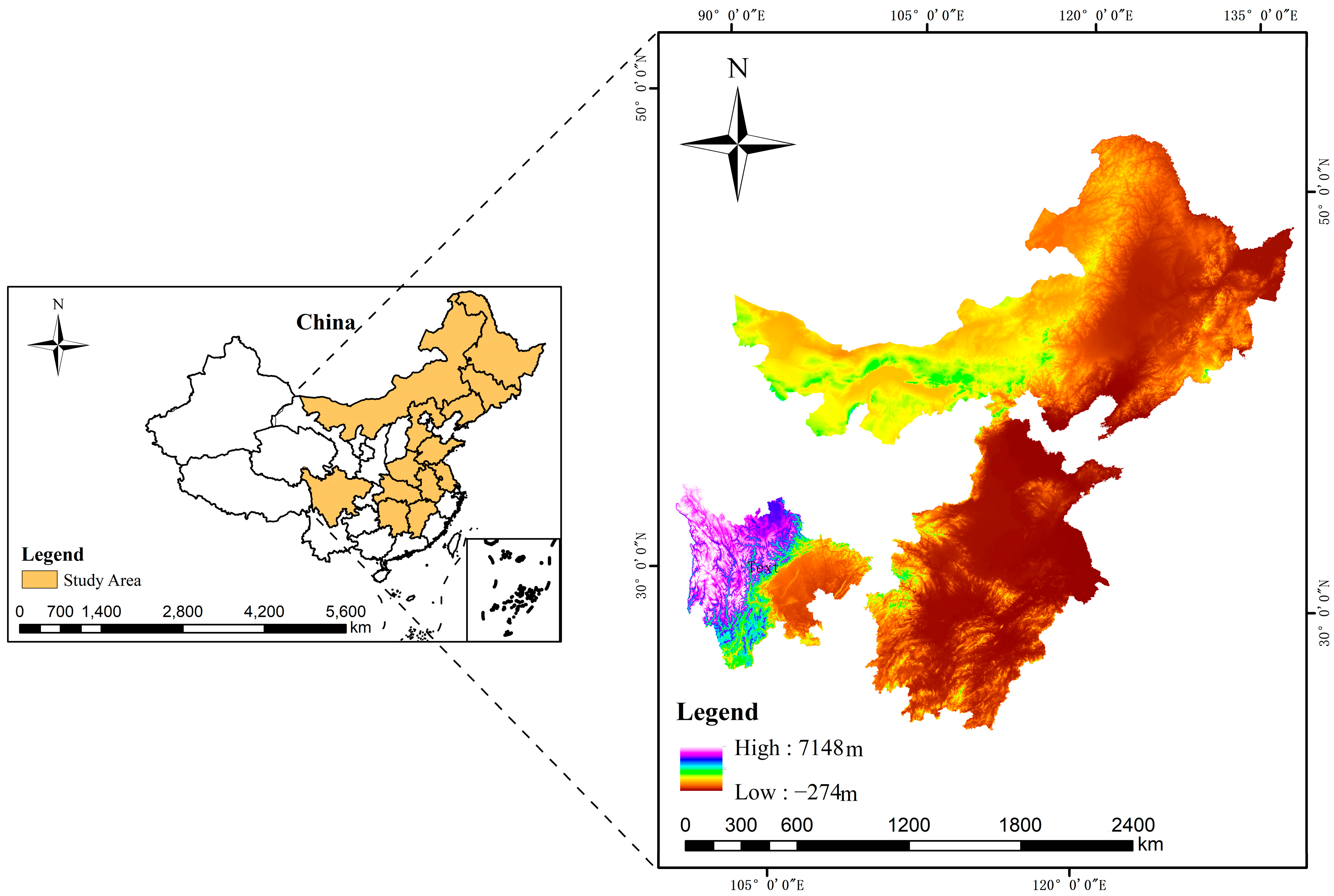
In 2003, the Chinese Ministry of Finance designated 13 provincial-level administrative regions—Inner Mongolia, Heilongjiang, Jilin, Liaoning, Hebei, Shandong, Henan, Jiangxi, Anhui, Jiangsu, Hubei, Hunan, and Sichuan—as MGPAs (as shown in Figure 2) [25]. In 2023, the per capita water resources in the MGPAs were 1.2 × 10 3   m 3 , which is only 62% of the national average standard of 2 × 10 3   m 3 , and is already in the “mild water scarcity” zone according to the United Nations standard. The total water supply in the MGPAs reaches 3.31 × 10 11   m 3 , of which the ratio of agricultural, industrial, living, and ecological water consumption is 0.607:0.190:0.141:0.062, with agriculture consuming the highest proportion of water resources, and the water consumption per CNY 10,000 of output value in the region is about 48   m 3 , which is 9% higher than the national average of 43.9   m 3 , indicating that there is still some space for water conservation. Overall, the total water resources of the MGPAs are about 9.25 × 10 11   m 3 , accounting for 35.9% of the national total 2.58 × 10 12   m 3 ; the total grain output is about 5.4 × 10 8   t , accounting for 78% of the national total 6.95 × 10 8   t . With less than 36% of the national water resources, 78% of the national grain output is supported, and there is significant pressure on water and land matching. In recent years, the center of grains in China has continued to move northward, and the over-concentration of grain production in some water-scarce provinces has aggravated the contradiction between the supply and demand of agricultural water [26]. Therefore, the assessment of the WRCC of MGPAs is conducive to the optimal use of water resources in the region and the alleviation of the contradiction between the supply and demand of water resources in the region.

3. Research Methods

3.1. Construction of Index System

The construction of an evaluation index system for WRCC is the core component of the entire evaluation process, requiring consideration of all relevant factors and their mutual influences. This paper focuses on the characteristics of MGPAs with large populations and an agricultural-based economy. Based on the foundational support role of water resources in human social production activities, their role in ensuring daily human life, and their critical role in maintaining ecological balance and meeting basic human ecological needs, an evaluation index system for water resources’ “production–living–ecology” (abbreviated as “three-life”) functions (see Table 1) is proposed, aiming to comprehensively reflect the value of water resources in sustaining socio-economic sustainable development and protecting the overall ecological functions of the environment [26].

3.2. Evaluation Criteria of Indicator Grades

The scientific and reasonable evaluation of WRCC depends not only on the selection of evaluation indicators but also on the grading standards of these indicators. Establishing scientific and reasonable grading standards for evaluation indicators is crucial to ensuring the accuracy and effectiveness of evaluation results. This study, based on the definition of WRCC, literature review, reference standards, expert opinions, and the actual conditions of the study area, categorizes WRCC indicators into five grades: Grade I—extremely low WRCC, Grade II—relatively low WRCC, Grade III—critical transition WRCC, Grade IV—relatively strong WRCC, and Grade V—extremely strong WRCC (see Table 2) [26,27,28]. The specific meaning is as follows:
Grade I: The region has sufficient water resources, with all indicators of WRCC well above warning levels. The available water supply is sufficient to meet the sustainable development needs of the “three functions” (production, living, and ecology), and the water resource system is in an ideal state.
Grade II: The region has relatively abundant water resources, with some indicators of WRCC approaching the development threshold. The available water supply basically meets the sustainable development needs of the “three functions” and still has potential for further development and utilization.
Grade III: Regional water resources are in a state of critical balance between supply and demand. Key indicators of WRCC have reached warning levels. Available water supply can still meet the sustainable development needs of the “three functions,” but it is insufficient to support regional sustainable development, and development potential has nearly reached its upper limit.
Grade IV: Regional water resources are clearly insufficient, key indicators of WRCC have exceeded warning levels, water resource development potential has exceeded sustainable thresholds, available water supply is insufficient to meet the sustainable development needs of the “three functions,” and the “three functions” are in a state of imbalance.
Grade V: The region suffers from severe water scarcity, with multiple indicators of WRCC exceeding warning levels. Water resource development intensity far exceeds sustainable thresholds, severely constraining the development of the “three functions” of the WRCC system. The water resource system faces enormous risks.

3.3. Data Sources

The raw data used in this paper are sourced from the China Statistical Yearbook, China Environmental Statistical Yearbook, China Rural Statistical Yearbook, and China Water Resources Bulletin from 2004 to 2023. Among these, the production function and living function indicators (C1, C2, C7, C9, C10, C11) are from the China Statistical Yearbook, the ecology function indicators (C12, C14, C16, C17) are from the China Environmental Statistical Yearbook, the production function and ecological function indicators (C4, C5, C6, C15) are from the China Rural Statistical Yearbook, and the remaining water use indicators (C3, C13) are from the China Water Resources Bulletin.

3.4. Determination of Indicator Weights

Existing research on weighting methods primarily employs single weighting approaches based on specific prior assumptions. Once actual indicator data deviate from these assumptions, the weights become systematically distorted, leading to invalid evaluation conclusions. To avoid these issues, this study employs a combined weighting method that integrates entropy weighting [29,30], mean square deviation, and CRITIC methods for weight calculation [31,32]. Entropy weighting reflects the dispersion of indicators, mean square deviation accounts for differences between indicators, and CRITIC integrates the correlation and conflict between indicators. The three methods, respectively, reflect the three dimensions of data dispersion, volatility, and association. By outputting weight intervals in parallel, they not only validate the robustness of single weighting but also provide multi-perspective evidence for subsequent combined weighting or sensitivity analysis, thereby enhancing the objectivity and robustness of evaluation results. The specific steps are as follows:

3.4.1. Indicator Raw Data Standardization

The min–max standardization method is used to linearly transform the raw data of each indicator, eliminating the impact of different units of measurement between indicators and ensuring that all indicators have consistent directionality when calculating weights, thereby better reflecting the relative strengths and weaknesses of the indicators [33].
Positive indicators: y i j = x i j min x j max x j min x j (1)
Negative indicators: y i j = max x j x i j max x j min x j (2)
where y i j is the standardized value of the j evaluation indicator in the year i ; x i j is the raw data of the j evaluation indicator in the year i ; and max x j and min x j are the maximum and minimum values of the j evaluation indicator in the evaluation year, respectively.

3.4.2. Entropy Weight Method

The entropy weight method is an objective weighting method based on information entropy. It reflects the degree of uncertainty of each indicator by calculating the information entropy value of each indicator. The calculation formula is as follows:
E j = 1 ln n i = 1 n p i j   ln   p i j
p i j = y i j i = 1 n y i j
d j = 1 E j
w e j = d j j = 1 m d j
where E j represents the information entropy value of the j th indicator; n is the number of samples; and p i j is the proportion of the standardized value of the i th sample on the j th indicator to the sum of the indicator. w e j denotes the entropy weight of the j th indicator; and m is the number of indicators.

3.4.3. Mean Square Deviation Method

The mean square deviation method, also known as the standard deviation method, is an objective weighting method based on statistical characteristics of data. It uses the variance of each indicator to measure its variability and reflect its relative importance in comprehensive evaluation. The calculation formula is as follows:
s j 2 = 1 n 1 i = 1 n y i j y ¯ j 2
w s j = s j 2 j = 1 m s j 2
where y ¯ j is the sample mean of the standardized value of the j evaluation indicator in the year i ; w s j indicates the weight of the mean-variance method of the j indicator; s j 2 is the variance of the j indicator; and m is the number of indicators.

3.4.4. CRITIC Method

The CRITIC method is an objective weighting method based on the strength of indicator comparisons and the conflict between indicators. This method determines the importance and weight of indicators by analyzing the interrelationships between them, enabling a more accurate assessment of the importance of indicators and providing a more comprehensive basis for decision-making. The calculation formula is as follows:
S j = 1 n 1 i = 1 n y i j y ¯ j 2
r j k = i = 1 n y i j y ¯ j y i k y ¯ k i = 1 n y i j y ¯ j 2 i = 1 n y i k y ¯ k 2 ( j k )
y ¯ j = 1 n i = 1 n y i j
R j = k = 1 n 1 r j k
c j = S j R j
w c j = c j j = 1 m c j
where y ¯ j is the sample mean of the standardized value of the j th evaluation indicator in the year i . r j k is the correlation coefficient between the j th indicator and the k th indicator; and y ¯ j and y ¯ k are the sum of the standardized values of the j th indicator and the k th indicator of the whole sample, respectively.

3.4.5. Combined Weights

The weighting for this project is determined by the average of the above three weights, using the following formula:
w j = 1 3 ( w s j + w e j + w c j )

3.5. Determination of WRCC

The indicators in the WRCC evaluation system are neither isolated nor simply linearly aggregated—they interact through nonlinear coupling, threshold transitions, and spatio-temporal lag, constraining and promoting each other, resulting in complex causal chains, feedback loops, and critical transitions within the system. This leads to high uncertainty and multi-stable characteristics in the pathways influencing WRCC. Neural network algorithms have simple data requirements and can accurately capture the nonlinear relationships in the complex, multi-element coupling of water resource systems. Through multi-layer nonlinear activation functions, they can precisely map the complex associations between environmental variables, avoiding the “overfitting” or “underfitting” phenomena that occur in traditional linear weighted models. Therefore, this paper selects the BP neural network algorithm to evaluate WRCC. Figure 3 shows the topological structure of the B-P neural network.

3.5.1. Training Sample Selection

Using the maximum and minimum values from the raw data of each indicator as the upper and lower limits, randomly generate a sample group (with 80% as the training set and 20% as the test set). The minimum value is estimated using the Vapnik–Chervonenkis Dimension, ensuring that each feature value in the sample is uniformly distributed within the specified range. If all evaluation indicators of a sample fall within the same grade interval, the WRCC grade of the sample is determined to be the corresponding grade. If the evaluation indicators fall within different grade intervals, the product of each indicator’s numerical value and its corresponding weight is divided into five equal parts from largest to smallest, corresponding to the five grades of the evaluation criteria, to determine the expected grade of the sample. The specific calculation process is as follows:
Generate N samples: x ( k ) = ( x 1 ( k )   , x 2 ( k )   , , x 17 ( k )   ) , k = 1 , 2 , , N
N V C ( H ) + log ( 1 / δ ) ϵ 2
(16)
g j ( k )   = G r a d e ( x j ( k )   ) { 1 , 2 , 3 , 4 , 5 } (17)
When the index grades are exactly the same, the following applies: g 1 ( k )   = g 1 ( k )     = = g 17 ( k )   = s     Grade ( x ( k ) ) = s (18)
When the indicator grades are not identical, the following applies: S ( k ) = j = 1 17 w C h i n a j × x j ( k ) min ( x j ( k ) ) max ( x j ( k ) ) min ( x j ( k ) ) (19)
S ( 1 )   S ( 2 )   S ( N ) (20)
G r a d e ( x ( k )   ) = 5 , S ( k ) S ( 1 ) , S ( N / 5 ) 4 , S ( k ) S ( N / 5 ) , S ( 2 N / 5 ) 3 , S ( k ) S ( 2 N / 5 ) , S ( 3 N / 5 ) 2 , S ( k ) S ( 3 N / 5 ) , S ( 4 N / 5 ) 1 , S ( k ) S ( 4 N / 5 ) , S N (21)
In Grade ( x ( k ) ) , x ( k ) represents the first k sample generated, x j ( k ) represents the j eigenvalue of the k sample, g j ( k )   represents the class of the j eigenvalue of the k sample, w C h i n a j represents the weight of the j eigenvalue of the whole country, S ( k ) represents the value of the weighted sum of all the indicators normalized to the k sample, S ( e ) represents the value of the weighted sum of all the indicators normalized to the e sample in S ( k ) in descending order, and e N represents the desired class of the water carrying capacity of the k sample. Where N represents the number of samples, V C ( H ) represents the Vapnik–Chervonenkis Dimension of the neural network, ϵ represents the tolerance of generalization error ( ϵ = 5%), and δ represents the confidence level ( δ = 0.05).

3.5.2. BP Neural Network Model Construction

A BP neural network is a unidirectional, multi-layer feedforward network consisting of an input layer, an output layer, and several hidden layers. There is no coupling between neurons within the same layer, and neurons between layers are connected via connection weights and thresholds. The learning process of a BP neural network is divided into two parts: forward propagation and backward propagation. Forward propagation inputs information, while backward propagation adjusts errors. During forward propagation, input information is transmitted forward to the neurons in the hidden layer, where it undergoes activation function operations before being transmitted to the neurons in the output layer. The actual output of the output layer and the expected output may have an error. When the error exceeds the specified threshold, the backward propagation process begins, where the error signal is transmitted back along the original path. By modifying the connection weights between neurons in each layer, the error is propagated sequentially back to the input layer, followed by another round of forward propagation. This process is repeated until the learning termination condition is met.
This paper selects a BP neural network algorithm with two hidden layers, uses the ReLU function as the activation function for the hidden layer neurons, does not use an activation function for the output layer, uses the cross-entropy loss function (nn.CrossEntropyLoss) combined with the softmax function to calculate the loss, uses the Adam optimizer for parameter updates, accelerates the training process through adaptive learning rates, and reduces the risk of overfitting. Specifically, the process is as follows:
(1)
Forward propagation process
I.
Input layer–the first hidden layer
The input layer receives the samples of evaluation indexes x , which are transmitted to the first hidden layer through the weight matrix W ( 1 ) and bias vector b ( 1 ) , and are activated by the activation function ReLU and then output. The formula is as follows:
z ( 1 ) = W ( 1 ) x + b ( 1 ) z 1 ( 1 ) z 2 ( 1 ) z 64 ( 1 ) = j = 1 17 W i j ( 1 ) x j + b i ( 1 )
a ( 1 ) = Re L U ( z ( 1 ) ) = max ( 0 , z ( 1 ) )
where x j denotes the normalized value of the first j evaluation index, W i j ( 1 ) denotes the weight of the first j index by the first i hidden neuron, b i ( 1 ) denotes the bias of the first i hidden neuron, z ( 1 ) denotes the net input of the first hidden layer, W ( 1 ) denotes the weight matrix from the input layer to the first hidden layer, b ( 1 ) denotes the bias vector of the first hidden layer, and a ( 1 ) denotes the activation vector of the first hidden layer.
II.
The first hidden layer–the second hidden layer
The output of the first hidden layer is transferred to the second hidden layer through the weight matrix, and the bias vector and is activated by the activation function ReLU. The formula is shown below:
z ( 2 ) = W ( 2 ) a ( 1 ) + b ( 2 ) z 1 ( 2 ) z 2 ( 2 ) z 32 ( 2 ) = j = 1 64 W i j ( 2 ) a j ( 1 ) + b i ( 2 ) a ( 2 ) = Re L U ( z ( 2 ) ) = max ( 0 , z ( 2 ) )
where z ( 2 ) denotes the net input of the second hidden layer, W ( 2 ) denotes the weight matrix from the first hidden layer to the second hidden layer, b ( 2 ) denotes the bias vector of the second hidden layer, and a ( 2 ) denotes the activation vector of the first hidden layer.
III.
Second hidden layer–output layer
The output of the second hidden layer a ( 2 ) is passed to the output layer through the weight matrix W ( 3 ) and bias vector b ( 3 ) , and the probability distribution is calculated using the softmax function. The formula is shown below:
z ( 3 ) = W ( 3 ) a ( 2 ) + b ( 3 ) z 1 ( 3 ) z 2 ( 3 ) z 5 ( 3 ) = j = 1 32 W i j ( 3 ) a j ( 2 ) + b i ( 3 )   y ^ = s o f t max ( z ( 3 ) ) = exp ( z ( 3 ) ) k = 1 5 exp ( z k ( 3 ) )
where z ( 3 ) denotes the net input of the output layer, W ( 3 ) denotes the weight matrix from the second hidden layer to the output layer, b ( 3 ) denotes the bias vector of the output layer, and y ^ denotes the probability distribution vector of the output layer.
(2)
Backpropagation process
In the backpropagation process, the gradient of the parameters of each layer is calculated by the chain rule, and the gradient calculation involves the gradient of the weight matrix and the bias vector. The error term for the output layer δ ( 3 ) is determined by the gradient of the loss function to the output layer, and the error term for the hidden layer δ ( l ) is calculated by the transpose of the weight matrix and the derivative of the ReLU function.
Error term of the output layer: δ ( 3 ) = y ^ y δ 1 ( 3 ) δ 2 ( 3 ) δ 5 ( 3 ) = y ^ 1 y 1 y ^ 2 y 2 y ^ 5 y 5 (26)
Error term of the hidden layer: δ ( l 1 ) = ( W ( l ) T δ ( l ) ) Re L U ( z ( l 1 ) ) (27)
Loss function: Re L U ( z ( l 1 ) ) = 1 z ( l 1 ) > 0 0 z ( l 1 ) 0 (28)
Weight gradient: L W ( l ) = δ ( l ) a ( l 1 ) T (29)
Bias gradient: L b ( l ) = δ ( l ) (30)
where y i c is the true label of the i th sample, and y ^ i c denotes the predicted probability that the i th sample belongs to the c th class. denotes element-by-element multiplication, and Re L U ( z ( l ) ) denotes the derivative of the Re L U ( z ( l ) ) function. δ ( l ) denotes the error term of the l th level, and l denotes the number of levels.
(3)
Parameter update
This paper uses the Adam optimizer for parameter updating. The Adam optimizer adjusts parameters through adaptive learning rate adjustment, combined with momentum and root mean square propagation. The formula is shown below:
Gradient first-order moment: m t ( θ ) = β 1 m t 1 ( θ ) + ( 1 β 1 ) L θ ( l ) (31)
Gradient second-order moments: v t ( θ ) = β 2 v t 1 ( θ ) + ( 1 β 2 ) ( L θ ( l ) ) 2 (32)
Bias correction: v t ( θ ) = β 2 v t 1 ( θ ) + ( 1 β 2 ) ( L θ ( l ) ) 2 (33)
Parameter update: θ ( l ) θ ( l ) α ( m ^ t ( θ ) v ^ t ( θ ) + ε ) (34)
where θ ( l ) denotes the parameter of layer l ( W ( l ) or b ( l ) ), α denotes the learning rate, m t ( θ ) denotes the momentum estimate at step t, v t ( θ ) denotes the second-order moment estimation of step t , β 1 denotes the momentum coefficients, β 2 denotes the root mean square decay coefficients, and ε denotes the smoothing term.

4. Results and Analysis

4.1. Identification of Factors Affecting WRCC Based on Weighting

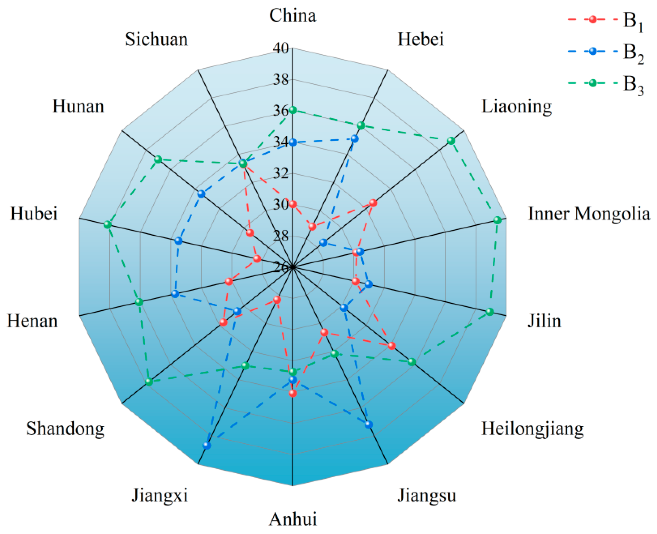
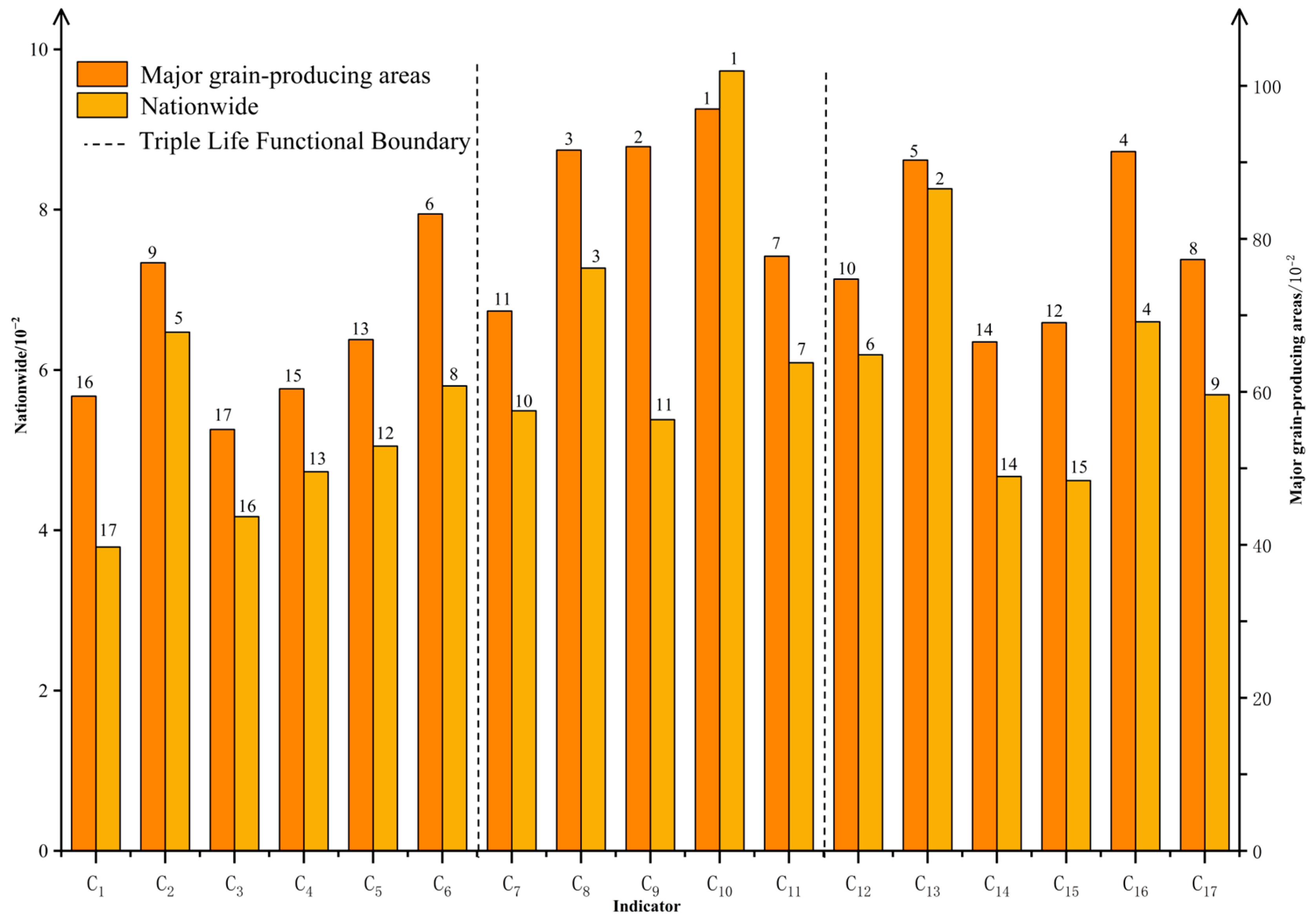
Substitute the actual data for each indicator from China and the 13 MGPAs from 2004 to 2023 into Formulas (1)–(5) to obtain the combined weights for each indicator (see Supplementary File). Based on the classification of indicators according to the “three-life” functions, the indicator weights of China’s 13 MGPAs were summed to obtain the weight distribution of the “three-life” functions for China and the 13 MGPAs (see Figure 4). The weights of the 13 MGPAs were summed according to the same indicators and compared with the national indicator weights to identify the primary difference indicators between the MGPAs and the national level that influence WRCC (see Figure 5).

4.1.1. Analysis of the Importance of the “Three Lives” Function in the Indicator System

As shown in Supplementary File, the weighting ratios of China’s water resources in the “three functions” are 30:34:36. The overall weighting distribution of water resources in MGPAs across the “three functions” exhibits a common characteristic of “ecology functions slightly dominant, followed closely by domestic functions, and relatively weaker production functions,” consistent with the national weighting distribution. This indicates that the distribution of the “three-life” functions of water resources in MGPAs does not differ significantly from the national distribution. Under the constraint of ensuring ecological water use, the primary focus is on meeting human daily water needs, followed by satisfying industrial and agricultural production water demands.
As shown in Figure 4, although the overall distribution of water resources in MGPAs is consistent with that of the country as a whole, differences in resource allocation, industrial structure, and population structure among administrative regions result in significant spatial heterogeneity in the distribution of the weightings of the “three functions” within these regions.
In terms of production functionality, nine administrative regions have indicator weights exceeding the national average (30.01%) among the 13 MGPAs, ranked as follows—Heilongjiang, Anhui, Sichuan, Liaoning, Shandong, Jiangsu, Henan, Inner Mongolia, and Jilin—with Heilongjiang having the highest weight, exceeding 4.08%. The remaining administrative regions all have weights below the national average, with Jiangxi having the lowest, at 1.69% below the national average. This is likely due to the fact that Heilongjiang, while being a MGPA, also has one of the highest levels of industrialization in the country. The high water consumption of both industry and agriculture in this region results in the highest production function weighting. The remaining eight administrative regions primarily rely on rice and wheat as their core crops, leading to high water resource demands for agricultural production and consequently higher production function weightings in these areas. Although Jiangxi primarily cultivates rice, its yield per unit area lags behind, and its level of industrialization is also not prominent, resulting in the lowest production function weight.
In terms of living functions, three administrative regions in the 13 MGPAs have indicator weights exceeding the national average (33.96%), accounting for over 23% of the total, and exhibiting a “higher in the south, lower in the north” pattern. Jiangxi in the south has the highest weight at 38.67%, while Liaoning in the north has the lowest at 28.49%, with deviations from the national average ranging between ±5.47%. This is directly related to population density and urbanization rates. In the south, the permanent population per square kilometer generally exceeds 500 people, and the urbanization rate exceeds 65%. Additionally, the average daily per capita water consumption is approximately 45 to 55 cubic meters, far exceeding the 35 to 40 cubic meters per day in northern regions. Therefore, the distribution of living function weights exhibits a “higher in the south, lower in the north” pattern.
From an ecology function perspective, the weight distribution of various indicators across the 13 MGPAs shows a pattern of “higher in the north and southwest, lower in the southeast,” with the ecology function weights of most provinces exceeding the national average of 36.03%. Only Jiangsu, Anhui, Jiangxi, and Shandong have weights below the national average. This is primarily due to the spatial distribution of precipitation in the study area. In the south, the average annual precipitation exceeds 800 mm, and there are numerous rivers and lakes, resulting in relatively low ecological water demand. Due to geographical location, the average annual precipitation in the north ranges from 400 to 600 mm, and evaporation rates are high, sometimes requiring artificial water supplementation to maintain ecological water demand. Meanwhile, since the beginning of the 21st century, the Chinese government has increasingly prioritized ecological conservation, implementing numerous important policies aimed at restoring the ecological environment in the north, leading to a higher distribution of ecological function weights in the northern regions.

4.1.2. Comparative Analysis of Key Indicators of WRCC in China and MGPA

By treating the 13 MGPAs as a whole, the combined weights of the same indicators are summed, ranked, and then compared with the national indicator weight rankings to analyze the differences between the MGPAs and the national WRCC indicators (see Figure 5).
As shown in Figure 5, the weights of each indicator are ranked from highest to lowest as follows: population density (C10), natural population growth rate (C9), per capita domestic water consumption (C8), Chemical Oxygen Demand Emission (C16), ecological water use rate (C13), irrigation coverage rate (C6), tertiary industry value added ratio (C11), ammonia nitrogen emissions (C17), the proportion of secondary industry added value (C2), agricultural water pollution index (C12), per capita GDP (C7), area of soil and water conservation (C15), water consumption per unit of grain production (C5), daily urban sewage treatment capacity (C14), water consumption per unit of agriculture output (C4), the proportion of primary industry added value (C1), and water consumption per unit of industrial output (C3).
In the national production function indicator system, the weight rankings of the proportion of secondary industry added value (C2), water consumption per unit of industrial output (C3), water consumption per unit of agriculture output (C4), and water consumption per unit of grain production (C5) are all significantly higher than those of the MGPAs. This phenomenon indicates that the industrial and agricultural production systems in the MGPAs have superior water use efficiency. Notably, the weighting rank difference for the secondary industry added value (C2) is as high as 4, highlighting that the driving effect of industrial structure composition on overall water efficiency is far stronger at the national level than in MGPAs. In industrial-dominated economies, water resource utilization efficiency is more easily constrained by industrial structure, while the agricultural production characteristics of MGPAs weaken the influence of industrial composition on regional water efficiency.
At the level of living functions, the weighting of per capita GDP (C7) is higher than that of MGPAs on a national scale, while the weighting of natural population growth rate (C9) is higher than that of MGPAs on a national scale. This indicates that economic levels dominate water consumption for living purposes, that water consumption for living purposes in MGPAs mainly meets basic needs and has a weak correlation with GDP, and that MGPAs face WRCC vulnerabilities caused by natural population changes.
From an ecology function perspective, only the daily urban sewage treatment capacity (C14) and chemical oxygen demand (COD) emissions (C16) have weighting rankings that are completely consistent with those of the national level and MGPAs. The agricultural water pollution index (C12) and ecological water use rate (C13) have weighting rankings that are higher at the national level than in MGPAs. Conversely, the area of soil and water conservation (C15) and ammonia nitrogen emissions (C17) are higher in MGPAs than at the national level. This indicates that at the national level, priority is given to addressing cross-regional common issues such as agricultural non-point source pollution and water ecology, while MGPAs, due to their core agricultural production functions, prioritize the protection of farmland water and soil resources and localized ammonia nitrogen pollution control to a higher degree.

4.2. BP Neural Network Model Training

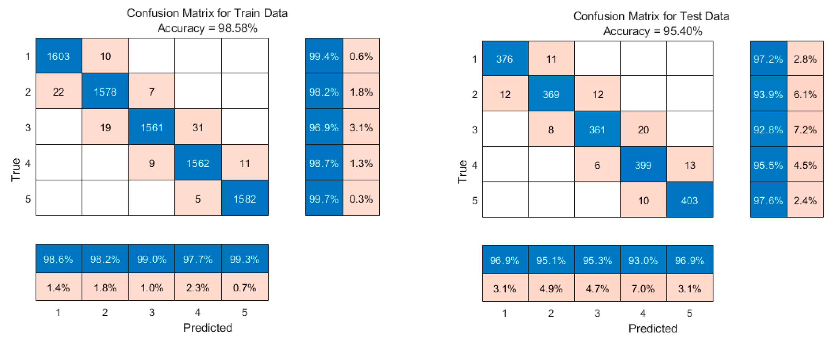
Based on the method for establishing the WRCC evaluation model described in this paper, the input layer and output layer of the BP neural network algorithm were determined to have seventeen dimensions and five dimensions, respectively, with the number of neurons in the two hidden layers set to 64 and 32, respectively. Based on the Vapnik–Chervonenkis Dimension theory (Formulas (16)–(21)), the sample size was determined to be 1 × 10⁴. Among these, 8 × 10³ samples were used for model training, and 2 × 10³ samples were used for model testing. The samples were input into the BP neural network model (see Formulas (22)–(34)). When the training and testing accuracy rates reached 98.58% and 95.40%, respectively (as shown in Figure 6), the iteration process was stopped, the internal parameters of the BP neural network algorithm were determined, and these parameters were used for the evaluation study of WRCC in the study area.

4.3. Evaluation and Analysis of WRCC in MGPA

The raw data for all evaluation indicators of WRCC in the 13 MGPAs from 2004 to 2023 were input into the trained BP neural network model, yielding the evaluation results for WRCC in the MGPAs (see Table 3). Years with significant changes in WRCC were selected as typical years, and the spatial distribution of WRCC in the study area was mapped (see Figure 7) to conduct a spatial variability analysis of WRCC in the MGPAs.

4.3.1. Analysis of Trends in WRCC

The changes in WRCC levels over time for the 13 MGPAs are shown in Table 3. During this period, the overall WRCC grades of the MGPAs remained at a relatively high level, with no province reaching Grade I, indicating that the sustainable water resource support capacity of the region urgently needs to be improved. Based on the patterns of changes in WRCC grades, the provinces can be categorized as follows:
WRCC grades continue to rise: Hebei, Liaoning, Inner Mongolia, Jilin, Heilongjiang, Jiangsu, Anhui, Jiangxi, Shandong, Henan, Hunan, and Sichuan. Among these, Inner Mongolia has seen a significant increase in its WRCC grade and faces relatively strong pressure. Due to its low irrigation coverage rate (13% lower than the national average) and low per capita domestic water consumption (8 m3 lower than the national average), its WRCC reached Grade IV as early as 2012. At this point, the water resources system was in a state of imbalance, barely able to maintain some functions, thereby constraining the development of the “three-life functions.” It remained stable at this grade for eight years before finally rising to Grade V in 2020. The WRCC grades of Shandong Province and Henan Province experienced a significant increase, with both provinces at Grade II in 2004 and rising to Grade V in 2019. At this point, the water resource system was in a severely imbalanced state and remained unchanged for five years. Due to Jiangxi Province’s irrigation coverage rate being 19% higher than the national average and its agricultural water pollution index being 0.6 t/104 m3 lower than the national average, it faced relatively less pressure, maintaining Grade II for 10 consecutive years from 2004 to 2013 and Grade III for 7 years from 2013 to 2020 and being the last province to reach Grade IV (in 2021).
WRCC grades experience fluctuating upward trends: Only Hubei Province exhibits a characteristic of overall upward trends with fluctuations in WRCC grades. Prior to 2011, the grade remained largely stable at Grade II, with the exception of a brief surge to Grade III in 2008, a year marked by poor ecological and environmental governance conditions, where the area of soil and water conservation was 6.8% lower than the average of other years and the daily urban sewage treatment capacity was 1.3% lower than the average of other years. After 2011, it remained at Level III for eight years, and in 2022, the carrying capacity further increased to Grade V.

4.3.2. Spatial Differences in WRCC

This study selected 2004, 2011, 2018, and 2023 as representative years. Based on the results of WRCC evaluations for provincial units in MGPAs, a spatial distribution map of WRCC grades was created (Figure 7) to reveal its spatial evolution patterns. In 2004, the MGPA were primarily classified as Grade II and Grade III, with Grade II accounting for 61.5% of the total, indicating a dominant position. The water resources system was in a state of tight supply–demand balance. WRCC grades in northern provinces were generally higher than those in southern provinces, resulting in a “north high, south low” spatial distribution pattern. In 2011, the spatial pattern continued to exhibit the “north high, south low” characteristic, but the dominant grade shifted to Grade III, accounting for 53.8%. At this point, the water resource system was in a state of critical supply–demand balance, with key indicators of the WRCC system approaching warning values, and development potential nearing its upper limit. Among these, Heilongjiang Province and Shandong Province were upgraded from Grade II to Grade III in 2004, while the grades of the remaining provinces did not undergo significant changes. In 2011, Heilongjiang Province’s water consumption per unit of agricultural output was 95.4% higher than the average of MGPAs, and its irrigation coverage rate was 20 percentage points lower than the average of MGPAs. This high-intensity agricultural water consumption, combined with lagging water-saving irrigation facilities, has further increased water resource pressure in Heilongjiang Province. In 2011, Shandong Province’s natural population growth rate was 1.1 percentage points higher than the average of MGPAs, its population density was three times the average of MGPAs, and its agricultural water pollution index was 1.7 times the average of MGPAs. Shandong Province’s high natural population growth rate has led to high population density, further exacerbating resource consumption, continuously increasing water demand, and causing the water resources system to operate beyond its capacity. In 2018, Grade II regions completely disappeared, with all provinces classified at Grade III or above. Grade IV became the dominant grade (accounting for 61.5%), and the water resources system as a whole was in a state of imbalance, barely able to maintain some functions, thereby constraining the development of the “three-life functions.” Sichuan Province remained at Grade III, while Henan Province and Jiangsu Province saw significant upgrades, rising from Grade II in 2011 to Grade IV, further highlighting the spatial heterogeneity of “higher in the north and lower in the south”. In 2023, Grade IV remained the dominant level (accounting for 61.5%), but Hubei Province experienced a significant leap, rising from Grade III in 2018 to Grade V, with the spatial pattern continuing to maintain a “north high, south low” configuration.

5. Discussion

5.1. Research Innovation

The study precisely targets 13 MGPAs critical to national food security. By constructing an evaluation system from a comprehensive perspective that integrates production, living, and ecology functions (“three-life” functions), it more fully characterizes the water resource system’s capacity to support the socio-economic and ecological composite systems in these regions. This provides a more systematic theoretical framework for scientifically assessing their water resource sustainability. In indicator weighting, we innovatively determine weights comprehensively across three dimensions—information dispersion, volatility, and conflict—overcoming the limitations of single-weighting methods and more objectively revealing the intrinsic information structure of indicator data. For hierarchical evaluation, the BP neural network algorithm with robust nonlinear fitting capability was introduced. To validate the accuracy and reliability of this model, cross-validation was conducted using the research findings from Zhao et al. based on Set Pair Analysis (SPA) and partial correlation coefficients (PCNs) [34]. Hebei, Shandong, Henan, and Inner Mongolia were classified as water-overloaded or significantly stressed regions in both studies. Zhao’s study indicates that these provinces exhibit a “negative development trend in WRCC systems,” consistent with our finding that most of these provinces were classified as Grade IV–V (severe water scarcity or overexploitation) in 2023. Through dynamic evolution analysis of partial correlation coefficients, Zhao further revealed that provinces like Jiangxi, Hubei, and Hunan show a “positive development trend” in WRCC, while Hebei, Inner Mongolia, and Shandong exhibit a “negative development trend”. This study further revealed through BP neural network long-term time series simulation that northern provinces (e.g., Inner Mongolia, Shandong, Henan) have experienced continuous deterioration in WRCC over multiple years due to low precipitation, high evaporation, and low agricultural water use efficiency, consistent with Zhao’s conclusion of “overloaded zones.” Southern provinces like Jiangxi and Hunan, despite their water resource advantages, have gradually escalated to Grade III–IV due to rising domestic and ecological water demands, further corroborating Zhao’s assessment of “generally sustainable zones with increasing pressure.” Despite differences in research methodologies, temporal scope, and indicator construction, both studies demonstrate high consistency and complementarity in evaluating WRCC across MGPAs. This indicates that neural network models exhibit strong robustness and predictive capability when addressing high-dimensional, nonlinear water resource system challenges.

5.2. Research Limitations

WRCC is a complex system involving multiple factors. This study constructed a relatively comprehensive integrated evaluation index system based on the “three lives” system framework, covering water resources, society, population, economy, and ecological environment. However, it is still necessary to point out the impact of some potential factors, such as changes in water prices, climate change, and policy changes, on the comprehensive utilization of water resources. The mechanisms of action of these factors and their systematic impact on the evaluation of WRCC can be further explored in subsequent studies. At the same time, this paper does not consider global WRCC. Compared with studies on China’s WRCC, research at the global level may hold greater significance.

5.3. Policy Recommendations

Based on an analysis of the evolution of WRCC grades in MGPAs from 2004 to 2023, it was found that the overall carrying capacity of the region has remained at a relatively high grade (Grade III and above) for a long time, with most provinces showing a sustained or fluctuating upward trend. The risk of systemic imbalance is prominent, severely constraining the coordinated development of the “three functions” (production, living, and ecology). To enhance the region’s sustainable water resource support capacity and ensure national food security and ecological security, the following policy recommendations are proposed:
For provinces where WRCC continues to rise, strict control should be exercised over the development of water-intensive industries, and policies such as “water-based production planning” and “water-based urban planning” should be implemented. For example, Inner Mongolia should prioritize improving irrigation coverage and water use efficiency. Shandong and Henan should mitigate the cumulative pressure on water systems caused by population growth and resource consumption, while strengthening pollution control and the development of a water-saving society. For provinces like Hubei, which exhibit fluctuating increases in WRCC, efforts should be made to enhance system resilience, establish a dynamic regulatory mechanism based on early warning indicators, and avoid the risk of system collapse caused by a sudden surge in WRCC within a short period. Water pollution control and ecological restoration should be jointly promoted. Agricultural non-point source pollution and industrial urban wastewater are key factors contributing to the degradation of water resource functions. We should draw on Jiangxi Province’s experience in achieving low pollution indices, promote ecological agriculture models, and reduce the use of fertilizers and pesticides. Given the spatial heterogeneity characterized by “higher in the north and lower in the south,” northern provinces should strictly control excessive groundwater extraction, promote inter-basin water diversion, and utilize non-conventional water resources. Southern provinces, although having relatively lower WRCC, should also guard against the risks of localized water quality deterioration and ecological degradation.

6. Conclusions

To investigate the sustainable development capacity of water resources in China’s MGPAs, this paper constructs a WRCC evaluation index system from the perspective of the “production–living–ecology” functions of water resources. It comprehensively applies the entropy weight method, mean square deviation method, and CRITIC method to combine and weight the indicators. to identify the weight distribution of the “three functions” and compare it with the national average. The main differences in indicators are analyzed, and a relationship network between the evaluation indicators and WRCC is constructed using a BP neural network model. The WRCC grades of each province within the MGPAs are determined, and their spatiotemporal variation characteristics are analyzed. The specific conclusions are as follows:
(1) The overall weight distribution of water resources in MGPAs in terms of the “three functions” is consistent with the national weight distribution, showing the common characteristics of “ecological function slightly dominant, living function close behind, and production function relatively weak.”
(2) Key indicators revealing the primary differences in WRCC between MGPAs and the national level indicate that, at the national scale, the proportion of industrial structure in production functions has a far stronger driving effect on overall water use efficiency than in MGPAs. In terms of living functions, economic levels dominate living water resource consumption, with living water use in MGPAs primarily meeting basic needs and showing weakened correlation with GDP. In terms of ecological functions, the national level places greater emphasis on cross-regional common issues, while MGPAs focus on their primary agricultural functions, elevating the protection of farmland water and land resources and localized ammonia–nitrogen pollution control to a higher priority.
(3) Over time, from 2004 to 2023, the WRCC grades in MGPAs have consistently increased. Northern provinces, characterized by low precipitation, high evaporation, and high agricultural water consumption, generally exhibit higher carrying capacity grades (IV–V). Southern provinces, though relatively abundant in water resources, still show an upward trend in ratings due to factors like population density and pollution pressure, albeit with a smaller increase and lower peak compared to the north. Spatially, the dominant grade shifted from Grade II (accounting for 61.5% in 2004) to Grade IV (also at 61.5% in 2023), maintaining a spatial pattern of “higher levels in the north and lower levels in the south.”
(4) Research reveals that China’s food security is highly dependent on water resource sustainability. However, WRCC in MGPAs has generally approached critical thresholds. Regional disparities between northern and southern areas, as well as differences between industrial and agricultural sectors, necessitate precise and differentiated policy approaches.

Supplementary Materials

The following supporting information can be downloaded at: https://www.mdpi.com/article/10.3390/agriculture15192074/s1, Table S1: Comprehensive Weights of Evaluation Indexes for WRCC in National and MGPA.

Author Contributions

K.C.: writing—review and editing, conceptualization, investigation, and funding acquisition. X.Z.: writing—original draft, methodology, visualization, data curation, and software. N.S.: project administration and supervision. All authors have read and agreed to the published version of the manuscript.

Funding

This research was funded by the National Natural Science Foundation of China (Grant No. 52179007).

Data Availability Statement

The raw data supporting the conclusions of this article will be made available by the authors on request.

Acknowledgments

Thanks to all authors for their efforts in conducting this research.

Conflicts of Interest

The authors declare no conflicts of interest.

Abbreviations

The following abbreviations are used in this manuscript:
WRCCwater resources carrying capacity
MGPAMajor Grain-Producing Areas

References

  1. Wang, J.; Li, Y.; Huang, J.; Yan, T.; Sun, T. Growing water scarcity, food security and government responses in China. Glob. Food Secur. Agric. Policy Econ. Environ. 2017, 14, 9–17. [Google Scholar] [CrossRef]
  2. Chen, Y.; Wang, J.; Zhang, F.; Liu, Y.; Cheng, S.; Zhu, J.; Si, W.; Fan, S.; Gu, S.; Hu, B.; et al. New patterns of globalization and food security. J. Nat. Resour. 2021, 36, 1362–1380. [Google Scholar] [CrossRef]
  3. Song, X.-M.; Kong, F.-Z.; Zhan, C.-S. Assessment of Water Resources Carrying Capacity in Tianjin City of China. Water Resour. Manag. 2011, 25, 857–873. [Google Scholar] [CrossRef]
  4. Li, Q.S.; Liu, Z.H.; Yang, Y.H.; Han, Y.; Wang, X.P. Evaluation of water resources carrying capacity in Tarim River Basin under game theory combination weights. Ecol. Indic. 2023, 154, 110609. [Google Scholar] [CrossRef]
  5. Lv, B.; Liu, C.; Li, T.; Meng, F.; Fu, Q.; Ji, Y.; Hou, R. Evaluation of the water resource carrying capacity in Heilongjiang, eastern China, based on the improved TOPSIS model. Ecol. Indic. 2023, 150, 110208. [Google Scholar] [CrossRef]
  6. Yang, H.; Sun, X.; Cheng, X.; Zhou, G.; Sun, G. Comprehensive evaluation of water resources carrying capacity in Weifang based on the VIKOR method. Acta Sci. Circumstantiae 2020, 40, 716–723. [Google Scholar]
  7. Yang, L.; Hao, Y.; Wang, B.; Li, X.; Gao, W. Evaluation of the water resources carrying capacity in Shaanxi Province based on DPSIRM-TOPSIS analysis. Ecol. Indic. 2025, 173, 113369. [Google Scholar] [CrossRef]
  8. Zhao, Y.; Wang, Y.Y.; Wang, Y. Comprehensive evaluation and influencing factors of urban agglomeration water resources carrying capacity. J. Clean. Prod. 2021, 288, 125097. [Google Scholar] [CrossRef]
  9. Liu, H.; Xia, J.; Zou, L.; Huo, R. Comprehensive quantitative evaluation of the water resource carrying capacity in Wuhan City based on the “human-water-city” framework: Past, present and future. J. Clean. Prod. 2022, 366, 132847. [Google Scholar] [CrossRef]
  10. Li, W.; Jiang, S.; Zhao, Y.; Li, H.; Zhu, Y.; Ling, M.; Qi, T.; He, G.; Yao, Y.; Wang, H. Comprehensive evaluation and scenario simulation of water resources carrying capacity: A case study in Xiong’an New Area, China. Ecol. Indic. 2023, 150, 110253. [Google Scholar] [CrossRef]
  11. Liu, L.; Yuan, X.; Jin, C.; Pan, C. Evaluation of water resources carrying capacity and development threshold in provincial capitals and typical cities of Northwest China. Arid. Zone Res. 2025, 42, 1–15. [Google Scholar]
  12. Anamaghi, S.; Behboudian, M.; Mahjouri, N.; Kerachian, R. A resilience-based framework for evaluating the carrying capacity of water and environmental resources under the climate change. Sci. Total Environ. 2023, 902, 165986. [Google Scholar] [CrossRef]
  13. Song, Q.R.; Wang, Z.C.; Wu, T.H. Risk analysis and assessment of water resource carrying capacity based on weighted gray model with improved entropy weighting method in the central plains region of China. Ecol. Indic. 2024, 160, 111907. [Google Scholar] [CrossRef]
  14. Tu, Y.; Han, W.; Zhang, E.; Li, H.; Ren, L.; Li, Q. Evaluation of water and soil resources carrying capacity based on the DPSIR-Cloud Model coupling: A case study of the irrigation area on the south bank of the Yellow River in Inner Mongolia. Arid. Zone Res. 2025, 42, 1–11. [Google Scholar]
  15. Qing, X.; Kan, Y. Study on forecast and regulation of water resources carrying capacity in Jiangsu Province based on GA-BP-SD coupling model. Water Resour. Hydropower Eng. 2022, 53, 86–99. [Google Scholar]
  16. Khorsandi, M.; Bateni, M.M.; Van Oel, P. A mathematical meta-model for assessing the self-sufficient water resources carrying capacity across different spatial scales in Iran. Heliyon 2023, 9, e15079. [Google Scholar] [CrossRef]
  17. Hadipour, M.; Pourebrahim, S.; Heidari, H.; Nikooy, F.; Ahmed, A.N.; Ern, C.J. Evaluation of water resource balance in the Urmia Lake Basin: Integrating carrying capacity and water footprint model for sustainable management. Ecol. Indic. 2024, 166, 112464. [Google Scholar] [CrossRef]
  18. Guo, X.; Chen, X.; Chen, Y.; Wang, R. Dynamic variation analysis of water resources carrying capacity in Xiamen City based on rough set theory and BP neural network. South-to-North Water Transf. Water Sci. Technol. 2015, 13, 236–240. [Google Scholar]
  19. Zhang, H.; Li, H.M.; Xu, X.Q.; Lv, X.B.; Peng, J.Y.; Weng, Q.R.; Wang, W.H.; Lei, K. Comprehensive assessment of the water environment carrying capacity based on machine learning. J. Clean. Prod. 2024, 472, 143465. [Google Scholar] [CrossRef]
  20. Xu, W.T.; Jin, J.L.; Zhang, J.Y.; Yuan, S.S.; Tang, M.; Liu, Y.L.; Guan, T.S. Prediction of regional water resources carrying capacity based on stochastic simulation: A case study of Beijing-Tianjin-Hebei Urban Agglomeration. J. Hydrol. Reg. Stud. 2024, 56, 101976. [Google Scholar] [CrossRef]
  21. Xie, C.Y.; Chao, L.; Shi, D.P.; Ni, Z. Evaluation of Sustainable Use of Water Resources Based on Random Forest: A Case Study in the Lishui River Basin, Central China. J. Coast. Res. 2020, 105, 134–136. [Google Scholar] [CrossRef]
  22. Chen, W.Z.; Chen, Y.; Feng, Y.Z. Assessment and Prediction of Water Resources Vulnerability Based on a NRS-RF Model: A Case Study of the Song-Liao River Basin, China. Entropy 2021, 23, 882. [Google Scholar] [CrossRef]
  23. Shi, C.Y.; Zhang, Z. A prediction method of regional water resources carrying capacity based on artificial neural network. Earth Sci. Res. J. 2021, 25, 169–177. [Google Scholar] [CrossRef]
  24. Das, A. An optimized approach for predicting water quality features and a performance evaluation for mapping surface water potential zones based on Discriminant Analysis (DA), Geographical Information System (GIS) and Machine Learning (ML) models in Baitarani River Basin, Odisha. Desalination Water Treat. 2025, 321, 101039. [Google Scholar] [CrossRef]
  25. Lee, C.-C.; He, Z.-W.; Luo, H.-P. Spatio-temporal characteristics of land ecological security and analysis of influencing factors in cities of major grain-producing regions of China. Environ. Impact Assess. Rev. 2024, 104, 107344. [Google Scholar] [CrossRef]
  26. Cheng, K.; Fu, Q.; Sun, N.; Wang, Z.; Zhao, Y. Comparative Analysis of the Evolutionary Characteristics and Influencing Factors of Land and Water Resource Systems in Major Grain-Producing Areas. Water 2023, 15, 2553. [Google Scholar] [CrossRef]
  27. Cheng, K.; He, K.X.; Sun, N.; Fu, Q. Comprehensive evaluation of eco-environmental resources in the main grain-producing areas of China. Ecol. Inform. 2023, 75, 102059. [Google Scholar] [CrossRef]
  28. Wang, T.Z.; Jian, S.Q.; Wang, J.Y.; Yan, D.H. Research on water resources carrying capacity evaluation based on innovative RCC method. Ecol. Indic. 2022, 139, 108876. [Google Scholar] [CrossRef]
  29. Wang, J.C.; Wang, Z.X.; Fu, Z.D.; Fang, Y.C.; Zhao, X.H.; Ding, X.; Huang, J.; Liu, Z.M.; Fu, X.H.; Liu, J.W. Spatial-Temporal Evaluation and Prediction of Water Resources Carrying Capacity in the Xiangjiang River Basin Using County Units and Entropy Weight TOPSIS-BP Neural Network. Sustainability 2024, 16, 8184. [Google Scholar] [CrossRef]
  30. Han, L.; Wang, Y.; Li, S.D.; Li, W.; Chen, X.J. Evaluation of Water Resource Carrying Capacity and Analysis of Driving Factors in the Dadu River Basin Based on the Entropy Weight Method and CRITIC Comprehensive Evaluation Method. Water 2025, 17, 2360. [Google Scholar] [CrossRef]
  31. Zhang, Y.M.; Gao, Y.; Zhang, Y.; Liang, Z.J.; Zhang, Z.L.; Zhao, Y.L.; Li, P. Assessment of agricultural water resources carrying capacity and analysis of its spatio-temporal variation in Henan Province, China. J. Clean. Prod. 2023, 403, 136869. [Google Scholar] [CrossRef]
  32. Cheng, K.; Zhu, B.; Sun, N.; Zhang, X.Y. Multi-Scale Spatiotemporal Characteristics Assessment of Water and Land Resources Ecological Security in China’s Main Grain-Producing Areas. Agriculture 2025, 15, 1770. [Google Scholar] [CrossRef]
  33. Bole, Y.; Rina, S.; Guga, S.; Na, M.; Fan, S.M.; Zhang, J.Q. Evaluation of resources, environment, and ecological carrying capacity from the perspective of “production-living-ecology” spaces: A case study of western Jilin Province, China. J. Clean. Prod. 2025, 491, 144770. [Google Scholar] [CrossRef]
  34. Zhao, W.; Wang, H.; Yang, Y.; Yan, J. Evaluation and Dynamic Evolution Analysis of Water Resources Carrying Capacity in Main Grain Producing Areas of China. Water Resour. Power 2021, 39, 56–60. [Google Scholar]
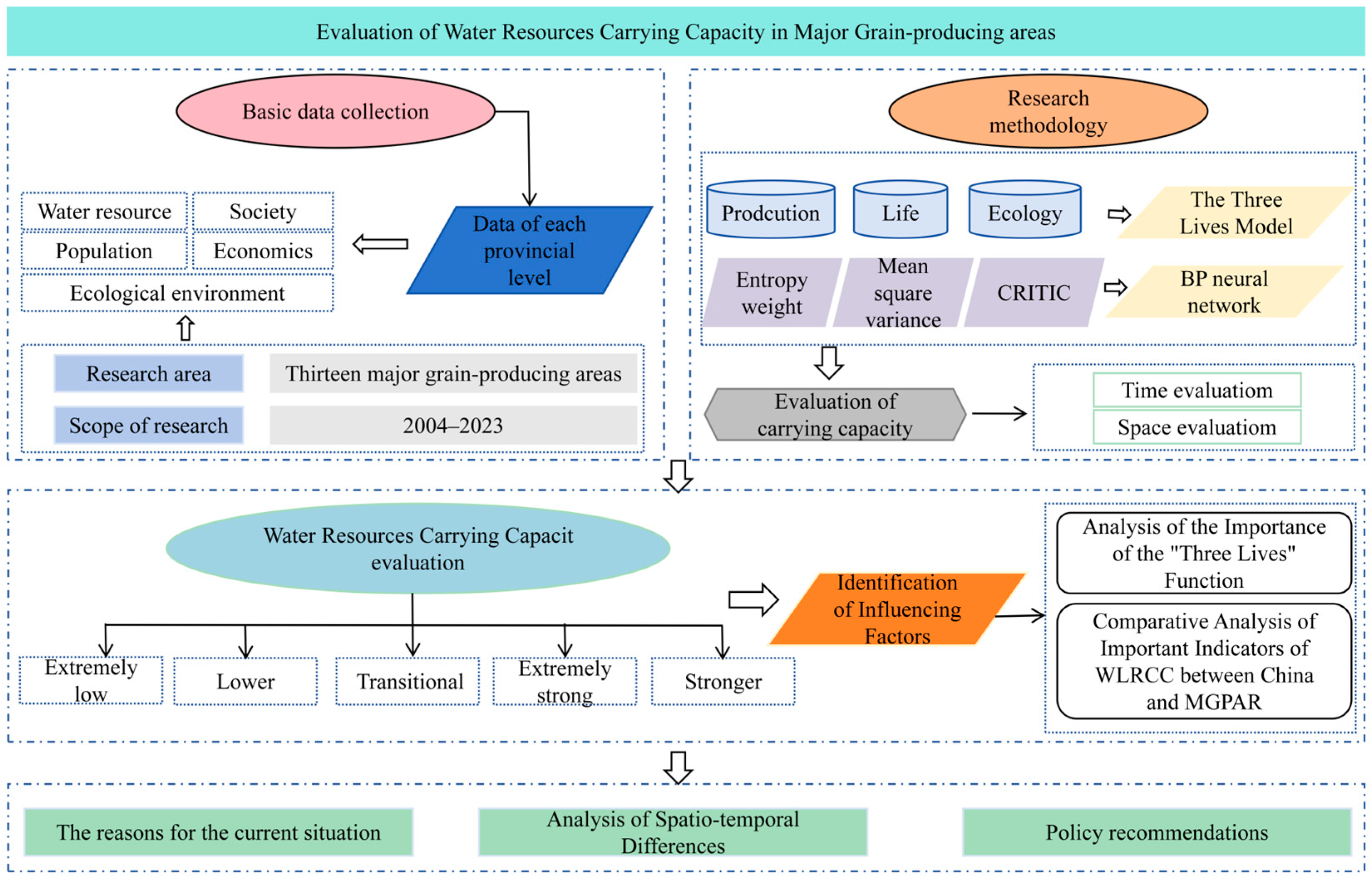
Figure 1. Research framework diagram.
Agriculture 15 02074 g001
Figure 2. Distribution of major grain-producing areas.
Agriculture 15 02074 g002
Figure 3. BP neural network topology diagram.
Agriculture 15 02074 g003
Figure 4. Weight distribution of the “three functions” of China and 13 MGPAs.
Agriculture 15 02074 g004
Figure 5. Weight distribution of indicators for evaluating WRCC in MGPAs.
Agriculture 15 02074 g005
Figure 6. Confusion matrix between neural network simulation values and actual values.
Agriculture 15 02074 g006
Figure 7. Spatial and temporal differences in the carrying capacity of water resources in MGPAs.
Agriculture 15 02074 g007
Table 1. Evaluation index system for water resource carrying capacity based on “production–living–ecology” functions.
Objective LayerCriteria LayerIndicator
Layer
UnitIndicator DescriptionAttribute
WRCCProduction function (B1)The proportion of primary industry added value C1%Primary industry output value/total output valuenegative
The proportion of secondary industry added value C2%Secondary sector output/total output valuenegative
Water consumption per unit of industrial output C3m3/yuanIndustrial water consumption/total industrial output valuenegative
Water consumption per unit of agriculture output C4m3/yuanAgricultural water consumption/total agricultural output valuenegative
Water consumption per unit of grain production C5t/104 m3Food production/water use in agriculturepositive
Irrigation coverage rate C6%Effective irrigated area/cultivated areapositive
Life function (B2)Per capita GDP C7104 yuanGDP/total populationpositive
Per capita domestic water consumptionC8m3Domestic water consumption/total populationnegative
Natural population growth rate C9%Annual net increase in number of people/total populationnegative
Population density C10Person/km2Total population/areanegative
Tertiary industry value added ratio C11%Ertiary industry output value/total output valuepositive
Ecology function (B3)Agricultural water pollution index C12t/104 m3Discounted use of fertilizers/agricultural water consumptionnegative
Ecological water use rate C13%Ecological water use/total water usepositive
Daily urban sewage treatment capacity C14104 m3Daily urban wastewater treatment capacitypositive
Area of soil and water conservation C15km2Soil erosion control areaPositive
Chemical Oxygen Demand Emission C16104 tChemical Oxygen Demand Emissionnegative
Ammonia nitrogen emissions C17104 tAmmonia Nitrogen Emissionnegative
Note: “positive” indicates that the larger the value, the better the indicator, while “negative” indicates that the smaller the value, the better the indicator.
Table 2. Classification criteria for evaluation indexes of water resource carrying capacity.
Target LayerCriteria
Layer
Indicator LayerGrading Criteria
Grade IGrade IIGrade IIIGrade IVGrade V
WRCCProduction function (B1)The proportion of primary industry added value C1<1010–1515–2020–30>30
The proportion of secondary industry added value C2<2525–3535–4040–55>55
Water consumption per unit of industrial output C3<0.0020.002–0.0050.005–0.0080.008–0.015>0.015
Water consumption per unit of agriculture output C4<0.030.03–0.070.07–0.10.1–0.2>0.2
Water consumption per unit of grain production C5>5035–5030–3520–30<20
Irrigation coverage rate C6>5540–5530–4025–30<25
Life
function (B2)
Per capita GDP C7>85–83–51–3<1
Per capita domestic water consumptionC8<3535–4545–5050–60>60
Natural population growth rate C9<22–3.53.5–55–6.5>6.5
Population density C10<100100–200200–400400–500>500
Tertiary industry value added ratio C11>7050–7040–5020–40<20
Ecology function (B3)Agricultural water pollution index C12<0.80.8–1.31.3–1.71.7–2.5>2.5
Ecological water use rate C13>63–61–30.5–1.0<0.5
Daily urban sewage treatment capacity C14>800600–800400–600200–400<200
Area of soil and water conservation C15>60,00050,000–60,00040,000–50,00020,000–40,000<20,000
Chemical Oxygen Demand Emission C16<3030–5050–8080–100>100
Ammonia nitrogen emissions C17<22–44–88–10>10
Table 3. Evaluation results of WRCC of MGPAs.
HebeiLiaoningInner MongoliaJilinHeilongjiangJiangsuAnhuiJiangxiShandongHenanHubeiHunanSichuan
2004IIIIIIIIIIIIIIIIIIIIIIIIIIIIIII
2005IIIIIIIIIIIIIIIIIIIIIIIIIIIIIII
2006IIIIIIIIIIIIIIIIIIIIIIIIIIIIIII
2007IIIIIIIIIIIIIIIIIIIIIIIIIIIIIII
2008IIIIIIIIIIIIIIIIIIIIIIIIIIIIIIIIII
2009IIIIIIIIIIIIIIIIIIIIIIIIIIIIIIIII
2010IIIIIIIIIIIIIIIIIIIIIIIIIIIIIIIII
2011IIIIIIIIIIIIIIIIIIIIIIIIIIIIIIIII
2012IIIIIIIVIVIIIIIIIIIIIIIIIIIIIIIIIII
2013IIIIIIIVIVIIIIIIIIIIIIIIIIIIIIIIIIII
2014IIIIIIIVIVIIIIIIIIIIIIIIIIIIIIIIIIIII
2015IIIIIIIVIVIVIIIIIIIIIIIIIIIIIIIIIIII
2016IIIIIIIVIVIVIIIIIIIIIIIIIIIIIIIIIIII
2017IVIVIVIVIVIIIIIIIIIIVIVIIIIIIIII
2018IVIVIVIVIVIVIIIIIIIVIVIIIIIIIII
2019VIVIVIVIVIVIIIIIIVVIIIIIIIV
2020VIVVIVIVIVIVIIIVVIVIVIV
2021VIVVIVIVIVIVIVVVIVIVIV
2022VIVVIVIVIVIVIVVVVIVIV
2023VIVVIVIVIVIVIVVVVIVIV
Disclaimer/Publisher’s Note: The statements, opinions and data contained in all publications are solely those of the individual author(s) and contributor(s) and not of MDPI and/or the editor(s). MDPI and/or the editor(s) disclaim responsibility for any injury to people or property resulting from any ideas, methods, instructions or products referred to in the content.