Abstract
With global warming, the increasing frequency of drought events threatens the stability of ecosystems, so the development of a rational ecological drought monitoring and assessment model is urgently needed. In this study, an evapotranspiration deficit (ED) was added for the first time into the construction of an ecological drought index. Considering atmospheric water deficit (WD), soil moisture (SM) and runoff (RF), both the Copula method and a nonparametric method were used to construct a multivariate comprehensive drought index (MCDI) to monitor ecological drought. The MCDI was evaluated using Pearson, actual drought validation, Theil–Sen, Mann–Kendall and ExtraTrees+SHAP methods, in order to assess differences between construction methods, analyze the drivers and sensitivities of ecological drought in Xinjiang, China, and specifically explore the role of ED in ecological drought. The results showed that (1) ED based on the ratio form is more suitable for capturing SM changes; (2) the performance of the composite drought index was improved in all aspects when cumulative effects were considered, and the ecological drought index based on the nonparametric method was superior to the index using the Copula method; (3) soil moisture was identified as the main contributor to ecological drought in Xinjiang, with the strongest synergistic effect occurring between SM and ED; and (4) the sensitivity of ecological drought to soil moisture within the arid regions increased nonlinearly along the decreasing SM gradient. In addition, the sensitivity to all drivers increased over time, with the largest increase observed for RF, followed by SM and then ED. The findings of this paper provide a useful reference for constructing a comprehensive drought index at the global scale, since the nonparametric method requires considerably fewer computational resources compared with the Copula method. In addition, the identified synergistic effect of ED and SM offers a new theoretical basis for ecological drought prevention and management in arid regions.
1. Introduction
Drought is a high-frequency natural disaster on a global scale that seriously threatens ecology, agricultural production, and socioeconomics [1,2]. In recent years, researchers have widely acknowledged the global warming trend and greening trend, and the problem of water scarcity is expected to become more prominent in the future. Ecological drought, which focuses on ecosystems and involves factors such as meteorology, soil, vegetation physiological status, and hydrological conditions [3,4,5], is characterized by an inadequate water supply within the ecosystem that fails to meet demand. This imbalance adversely affects the services provided by ecosystems and may trigger feedback processes in both natural and human systems [6,7]. Numerous studies have demonstrated the growing risks related to the global atmospheric water cycle, runoff recovery, soil water stress, and plant productivity [8,9,10], and projections suggest that the risk of future ecological droughts will continue to increase.
In order to scientifically protect ecosystems from drought damage, a comprehensive and accurate assessment of the degree of drought is essential. Due to the complexity of the causes of ecological drought, a multivariate composite drought index reflects ecosystem water stress more comprehensively than a single-variable index [11]. Clarifying the potential formation mechanisms of ecological drought is crucial for selecting appropriate drought indices. Ecological drought is a process in which the precipitation deficit in the early stage propagates to the soil, hydrological, and vegetation systems, and eventually develops into the whole ecological water stress [5]. Early comprehensive (composite) drought assessments combined precipitation with soil moisture or runoff [12,13,14] to evaluate meteorological, agricultural, or hydrological drought. Since then, studies have shown that evapotranspiration contributes to drought formation by regulating the water cycle [15], e.g., increased evaporative demand from the atmosphere and increased transpiration from vegetation exacerbate soil water deficit. At the same time, composite indices that consider rainfall but not ET may lead to biased assessments of drought intensity [16,17,18]. Therefore, the evapotranspiration factor or standardized precipitation evapotranspiration index (SPEI) has been commonly used as a meteorological factor in ecological drought [19] Other researchers [20,21] have included vegetation physiological indicators in ecological drought assessments, such as solar-induced chlorophyll fluorescence (SIF) and gross primary production (GPP) [5,22]. So far, researchers have generally considered five categories of factors within integrated drought assessment, including meteorological (precipitation and evapotranspiration), soil moisture, hydrological (surface runoff and subsurface runoff), and vegetation physiological indicators (SIF, GPP, etc.) [3,5].
Several researchers have pointed out the need to consider evapotranspiration deficit (ED) in future agricultural and ecological drought studies, since ED can better explain physical and physiological processes during drought [23]. However, less is known about the application of ED in integrated ecological drought assessments and the role it plays. ED indices were initially developed to monitor sudden droughts and to better capture the dynamic response of plants to water stress in crop areas with limited water resources, compared with vegetation indices or meteorological drought indices such as SPEI [24]. It is worth noting that there is a nonlinear decoupling between AET and AED [25], which is related to the coupling effects among soil, vegetation, and atmosphere [26,27]. Usually, AET first increases in the same direction as AED, but as SM and atmospheric moisture decline, drought persistence leads to decreasing plant stomatal conductance and reduced AET, or even to a complete decoupling of AET and AED [28]. In addition, during drought development, the decoupling of AET and AED occurs before visible changes in vegetation morphology [26]. Therefore, integrating ED into composite drought indices can enable rapid monitoring of ecological drought occurrence [29].
Ecological drought is a multi-system moisture deficit process, with temporal differences in drought propagation between systems. Numerous studies have analyzed the cumulative time effects of meteorological drought. For example [30,31], the 3- to 6-month SPEI is strongly correlated with changes in soil moisture [32,33], and the response time of soil moisture to meteorological drought is longer at greater soil depths (time scales) [34]. In addition, SPEI time scales are usually longer in irrigated areas than in dry farming areas [35]. Other scholars found that the evaporative demand index (SEDI) showed stronger correlations with crop yield at different cumulative time scales compared with other drought indices [36]. Overall, composite drought indices that consider cumulative effects maintain good correlations with meteorological, hydrological, soil, and vegetation factors [37,38], However, there is still a lack of systematic understanding of how cumulative drought effects are manifested in ecological droughts in Xinjiang.
After understanding the main impact indicators of ecological drought and their cumulative effects, it is also very important to choose a suitable method for constructing the comprehensive index. The construction methods of comprehensive drought index mainly include linear method and nonlinear method. The linear method mainly relies on weight setting, which usually includes the use of entropy weighting and principal component analysis [39,40]. However, this method is highly subjective and fails to capture the complex nonlinear response relationships among elements [3,4]. For example, some studies have shown that vegetation will first close stomata to reduce evapotranspiration under a certain drought stimulus, but once a threshold is exceeded, plants may reopen stomata to accelerate the evaporation of soil moisture [41,42]. Among nonlinear methods, the Copula function has become a favored approach for integrating multidimensional drought factors because it is not constrained by marginal distribution functions and can link drought factors with different time-varying characteristics. With this method, all types of standardized indices can be directly combined into a composite drought index [3,43]. In addition, nonparametric methods (e.g., Gringorten location maps) have gradually emerged in the arena of drought assessment methods. These methods do not require assumptions about model parameters and are easy to construct, while Copula function methods suffer from difficulties in high-dimensional solutions [4,38]. Many researchers have supported the use of Gringorten location maps to simplify the calculation of composite indices. However, the differences between drought indices obtained by the Copula and Gringorten methods are still unknown.
There are numerous cases of comprehensive drought indices to monitor and assess agricultural/ecological droughts; however, most of the current drought mechanism studies are on single or two-factor droughts, and studies on the driving mechanism of multifaceted comprehensive droughts are still scarce. Early studies on the driving mechanisms of drought considered rainfall deficit as the primary cause [15]. With advances in drought research, there is now general consensus among researchers that evapotranspiration (ET) is of great importance in the terrestrial air–water cycle and that atmospheric evapotranspiration demand (AED) will become increasingly important in future droughts [23,44,45]. The results of related studies show a global trend of increasing drought severity, to which AED contributes on average 40% [45]. Soil moisture (SM) anomalies are one of the main drivers of ecological drought, and many researchers have conducted extensive studies on the role of soil moisture. After drought exposure, the total primary productivity of forests becomes significantly more sensitive to subsequent water stress [46]. The effect of soil moisture on vegetation productivity is even more critical under compound extreme droughts (soil moisture-meteorology) [47]. Vegetation sensitivity to SM increases in dry climates [48], and vapor pressure deficit (VPD) is the main driver influencing SM changes [49]. Compared with VPD, SM stress has a greater effect on vegetation productivity, while the synergistic effect of VPD and SM is the most dominant interaction [50]. In addition, some studies have shown that under future scenarios, rainfall and VPD contribute less to future drought, while temperature anomalies exacerbate drought [51].
Xinjiang Uygur Autonomous Region, located in Northwest China, is characterized by uneven spatial distribution of precipitation and high evapotranspiration rates [52,53]. The frequency and severity of droughts in the region will increase in the future due to the influence of global warming [54]. In this study, based on the selection of WD, SM and total runoff (RF), ED was introduced as an indicator of ecological drought for the first time. A comprehensive drought index model was constructed using both Copula and nonparametric methods, taking into account the unique cumulative drought effects in Xinjiang, and the performance of the index was evaluated. Finally, using the machine learning ExtraTrees+SHAP, in which several important previously identified factors were added, the driving mechanisms of ecological drought were analyzed. The objectives of this study are as follows: (1) to analyze the cumulative drought effects of meteorological, hydrological, and evapotranspiration deficits, and to determine the time scales of each factor; (2) to construct a comprehensive ecological drought index (MCDI) based on Copula and nonparametric methods and compare the index performances; and (3) to explore the driving mechanisms of ecological drought in the region.
2. Study Area and Data Sources
2.1. Study Area
Xinjiang (73°40′–96°18′ E; 34°25–48°10′ N) is located on the northwest border of China, covering a total area of approximately 1.6649 million km2. It is a major arid and semiarid region in China (Figure 1), characterized by the presence of different land use types, including bare land, grassland, and farmland. On the other hand, the Xinjiang region has a typical temperate continental climate, with substantial spatial variations between the northern and southern parts. Indeed, the average annual temperature in the northern and southern parts of Xinjiang ranges from −4 to 9 °C and 7 to 14 °C, respectively. Similarly, the annual precipitation in the northern part of the region ranges from 100 to 500 mm, exceeding that in the southern part (<100 mm) and, consequently, making water resources in this part scarce.
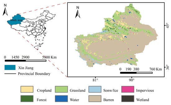
Figure 1.
Geographic location and land use types of the study area.
2.2. Data Sources
For the study period 2001–2022, monthly datasets of precipitation (PRE) were obtained from MSWEP (https://www.gloh2o.org/mswep/#faq (accessed on 1 March 2024)) with a spatial resolution of 0.1°. Potential evapotranspiration (PET), actual evapotranspiration (AET), and soil moisture (SM) monthly datasets were obtained from GLEAM (https://www.gleam.eu/ (accessed on 4 August 2024)) with a spatial resolution of 0.1°. Monthly datasets of runoff (RF), surface temperature (TMP) and dew point temperature were obtained from ERA5-land (https://cds.climate.copernicus.eu/ (accessed on 10 April 2024)) with a spatial resolution of 0.1°. Monthly data on normalized vegetation index (NDVI) were obtained from National Earth System Science Data Center (https://www.geodata.cn/ (accessed on 15 April 2024)) with a spatial resolution of 1 km. Monthly data on gross primary productivity (GPP) were obtained from the monthly scale GOSIF GPP dataset (https://globalecology.unh.edu/data/GOSIF-GPP.html (accessed on 26 April 2024)) with a spatial resolution of 0.05°. Finally, all data were resampled to 0.25° using bilinear interpolation.
3. Methods
3.1. Aridity Index (AI)
The aridity index (AI) is based on the fact that P and PET measure water supply and demand, respectively. Whereas P-to-PET ratios can reflect water supply and demand degrees, providing insights into the aridity or wetness of climatic conditions in a given year [55,56,57]. This index is, in fact, commonly used to define climate types (Table 1), according to the World Atlas of Desertification published by the United Nations Environment Programme (UNEP) in 1992 [58]. The AI values can be calculated using the following formula:
where MA_P and MA_PET denote the mean multi-year precipitation and mean multi-year potential evapotranspiration values, respectively.

Table 1.
Classification of climate types according to AI values.
3.2. Standardized Drought Index (SDI)
SPEI, SEDI, SSI, and SRI at different time scales are calculated by referring to the description of SPEI calculation by Vicente-Serrano [44], and the water deficit (WD), evapotranspiration deficit (ED), soil moisture (SM), and total runoff (RF) of the hydrometeorological indexes at different time scales are considered as the variables D for standardization, respectively, and it should be noted that WD is the difference between rainfall and potential evapotranspiration, ED is the ratio of actual evapotranspiration to potential evapotranspiration, and RF is the sum of surface and subsurface managers. Distribution functions such as norm, genextreme, beta, weibull_min, and pareto were chosen to fit the monthly series values of D. The largest R2 value of each distribution function was chosen as the current distribution function for each grid point, and the empirical cumulative probability value CDF was calculated, and finally the four standardized indices were derived using the inverse normal function as follows:
where P is the CDF value corresponding to a certain value of D and is the inverse function of the normal distribution function. The SDI drought thresholds are shown in Table 2.
Table 2.
Classification of drought types.
3.3. Copula Method to Construct a Quadratic Drought Index
Before calculating the multivariate composite drought index MCDI, we calculated the monthly scale SSI and the 1-, 3-, 6-, 9-, and 12-month scales SPEI, SEDI, and SRI according to the Section 3.2. The pre-cumulative effects are considered. Based on the maximum Pearson correlation coefficient between SSI and SDIi (i = 1,2, …, 12), the maximum r value is regarded as the optimal pre-cumulative drought effect of the time scale, and the three optimal time scale indices obtained were denoted as SPEIn, SEDIn, and SRIn, respectively. Meanwhile, in order to validate the superiority of the composite indices that took into account the pre-existing cumulative effects, we used the one-month time scale SPEIo, SEDIo, SRIo, and SSI as the control group. Then, based on the cumulative distribution function values CDF of SPEI, SEDI, SSI, and SRI for the corresponding time scales in both cases of considering the prior cumulative effect and not considering the prior cumulative effect, we selected the four most widely used Copula, Clayton, Frank, Gumbel, and Gaussian for constructing the joint distribution. Using the great likelihood method to estimate the parameters of different Copula, and using the AIC and BIC criteria to select the optimal Copula function model, we obtained the value of Copula value for the joint probability of the four indexes P. Finally, we obtained the quadratic composite eco-index MCDI by inverse standardization of P.
where P is the joint probability value of WD, ED, SM, and RF, and is the inverse function of the normal distribution function. The drought thresholds for MCDI are the same thresholds used for MCDI as for SDI since the selected SPEI, SEDI, SSI, and SRI have the same thresholds (Table 2).
3.4. Nonparametric Method for Constructing a Quadratic Drought Index
Cases of the nonparametric joint distribution method Gringorten for constructing the composite drought index are still scarce, and the difference in results compared to Copula is still unknown. Therefore, we use Gringorten to construct MCDI, consistent with the treatment in Section 3.3, the construction of the joint probability using Gringorten’s formula is carried out under the two cases of considering the pre-cumulative effect and not considering the pre-cumulative effect, using the SPEI, SEDI, SSI, and SRI under the same conditions as those in Section 3.3, as follows:
where is the total number of observations. , , , and stand for SPEI, SEDI, SSI, and SRI, respectively. mi is the frequency that simultaneously satisfies ≤ , ≤ , ≤ , and ≤ (1 ≤ ≤ ), and finally the MCDI is obtained by using the same inverse standard Equation (3).
3.5. Extra Trees+SHAP Contribution Analysis
SHapley Additive exPlanations (SHAP) provides a methodology for interpreting machine learning models (models about trees) by assigning importance to features through cooperative game theory. A SHAP value is computed for each feature indicating its relative contribution to the model predictions, suitable for model interpretation in the presence of complex multifactorial effects. ExtraTrees is a machine learning algorithm based on integrated learning, specialized for regression problems. It is a variant of Random Forest, and the core idea is to construct multiple decision trees and average their predictions to obtain the final prediction, so as to improve the generalization ability and robustness of the model.
Tree-based ensemble models (such as random forests and extreme random trees) are inherently robust to multicollinearity. The reasons are as follows: (a) Feature selection mechanism: when constructing each tree, the algorithm will avoid two highly correlated features appearing at the same node, or select the one with the largest information gain for splitting. (b) Not dependent on the linear hypothesis: The tree model is based on the ‘if-then’ condition judgment, and the tree model does not calculate the coefficients in the linear hypothesis. (c) The average effect of ensemble learning: Extremely random trees work by building a large number of trees and averaging their results (for regression) or voting (for classification).
In this study, the parameter space automatic optimization method is used in the model, and the model result with the largest R2 among all parameter combinations is taken as the final model. The SHAP calculation formula is as follows in Equation (5).
where S(x) is the MCDI value obtained by the model, is the predicted average MCDI value, and is the SHAP value of a characteristic variable.
3.6. Correlation Analysis
Pearson correlation coefficient (r) was used to calculate the correlation of each index with SM, NDVI, and GPP. A value of r less than 0 indicates a negative correlation and greater than 0 indicates a positive correlation, and the absolute value of r was used as the correlation strength to compare the magnitude of the correlation.
3.7. Theil–Sen Estimator
The Theil–Sen estimator does not depend on a particular data distribution and is insensitive to errors and extreme values in data. This method takes the median of data pair slopes of all samples to determine changing trends in time series, making it a robust nonparametric statistical method [59]. The Theil–Sen estimator can be computed using the following equation:
where β denotes the median of data pair slopes; Median denotes the median function; xi is the ith item in the time series; and xj is the jth item in the time series.
3.8. Mann–Kendall Trend Test
The Mann–Kendall test (M-K test) is a very robust nonparametric statistical test used to test the statistical significance of trends. This method does not require specific data distributions (e.g., normal distribution). Moreover, the M-K test results are not affected by missing values and outliers [60]. This method can be expressed by the following equation:
where n denotes the number of samples, xi is the ith item in the time series; xj is the jth item in the time series; sgn() is the sign function, which can be calculated as follows:
when n < 10, the trend test is performed directly using the S equation. If n > 10, S is standardized using the Z-score method, according to the following equations:
4. Results
4.1. Applicability of EDr and EDd
There are two main forms of evapotranspiration deficit indices: one is the ratio of actual evapotranspiration (AET) to potential evapotranspiration (PET) (EDr), and the other is the difference between the two (EDd). To quantify the differences between these two forms of drought discrimination, Pearson correlations were calculated for EDr and EDd with surface soil moisture (SMs) and root zone soil moisture (SMr), respectively. Based on the spatial distribution patterns of the correlations (Figure 2), EDr showed a wider range of positive correlations, while correlations with SMs were significantly stronger than those of EDd. In terms of average correlation values, the correlations of EDr and EDd with SMs were 0.67 and 0.59, respectively. For SMr, the average correlation values for EDr and EDd were 0.62 and 0.52, respectively. Across different land use types (Figure 1), the two EDs showed higher correlations in barren and grassland areas. However, EDd showed a poor negative correlation in some wetter forest areas, whereas EDr generally showed better adaptability to a wider range of vegetation types.
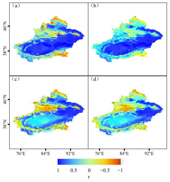
Figure 2.
Correlation of EDr (a,b) and EDd (c,d) with SMs and SMr, respectively (p < 0.05, time scale is 1 month).
We further quantified the proportion of vegetation contributing to actual evapotranspiration using the ratio of vegetation transpiration to actual evapotranspiration (VTA). When the ratio is small, evapotranspiration is dominated by surface evapotranspiration, with surface soil moisture being the main source of evapotranspiration. By analyzing the mean values of correlation between SM and EDr or SM and EDd for different ranges of ratios (Figure 3), we found that mean correlation curves of EDr with SMs and SMr were consistently above those of EDd, indicating that EDr was more suitable for different ranges of VTA in the study area. In addition, as mean VTA decreased, both mean SMs and SMr decreased, and at the same time the correlations between SMs/SMr and EDr/EDd became stronger. However, in areas with the highest VTA and SMs/SMr, correlations fell below 0.2.
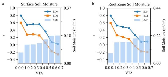
Figure 3.
Correlation of EDr-SM (a) and EDd-SM (b) under different VTAs.
Overall, EDr better captured soil moisture variability in the study area compared with EDd. It is noteworthy that the ET deficit index performed better in regions with low VTA (sparsely vegetated). However, the evapotranspiration deficit index may not be able to adequately explain soil moisture variability in high VTA areas (densely vegetated and wetter climates). The better performance of EDr may be attributed to the ratio form narrowing the data scale, thus reducing error. On the other hand, with an array range of 0–1 for both soil moisture and EDr, EDr responds more quickly to changes in SM. Therefore, EDr was finally chosen as the calculation method for the ED indicator. In addition, compared with the correlation between EDr and SMr, there were some regions (0.1 < VTA < 0.4) where the correlation between EDr and SMs was higher. Thus, when considering the role of soil moisture in different layers, the soil moisture layer that has a stronger correlation with EDr serves as the optimal soil moisture value (SMn) for that image point.
4.2. Determining the Optimal Time Scale for the Cumulative Effects of the Preceding Period
Considering the pre-cumulative effects of water deficit (WD), evapotranspiration deficit (ER), and runoff (RF), Pearson correlation coefficients (r) were calculated between SPEI, SEDI, and SRI at different time scales (months) and SSI (in SMn), respectively. The time scale with the highest correlation was taken as the optimal time scale. The magnitudes of the correlations with SSI and the spatial distribution of the specific time scales for the three drought indices (SPEIn, SEDIn and SRIn) are shown in Figure 4. The average correlations for SPEIn-SSI, SEDIn-SSI, and SRIn-SSI are 0.53, 0.72, and 0.39, respectively. In the case of SPEIn-SSI, SPEIn showed high correlations (r > 0.7) mainly in the fringe, northern and eastern regions, with the optimal time scale dominated by 3 months (41.1% of the area). In contrast, the southwestern part of the study area was dominated by the 1-month scale. SEDIn showed high correlations (r > 0.7) mainly in the southern, northwestern and eastern regions, with the optimal time scale dominated by 1 month (71.3% of the area). Areas with an optimal time scale greater than 1 month were mainly located along the northern and southern edges and in the west. SRIn showed high correlations (r > 0.7) mainly along the southwestern, western and northern edges, with the optimal time scale dominated by 1 month (42.9% of the area). Interestingly, part of the eastern region had 12 months as the optimal time scale, though the correlation was lower than 0.1.
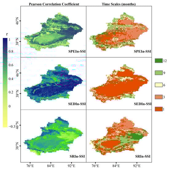
Figure 4.
Correlation of SPEIn, SEDIn and SRIn with SSI, respectively.
Further analysis examined temporal trends in the correlations between SPEIn, SEDIn, SRIn, and SSI across Xinjiang (Figure 5), with regions classified by aridity index (AI) (Table 1). The Theil–Sen estimator was used to calculate the slopes of the mean correlation trends, and the Mann–Kendall test was used to assess their significance. The results revealed a significant decreasing trend in the SPEIn-SSI correlation. This decline was particularly pronounced and statistically significant in regions classified as Semi-Arid to Hyper-Arid. Conversely, Dry Sub-Humid to Humid regions exhibited a contrasting, albeit non-significant, pattern with a tendency towards increasing correlation. For SEDIn, correlations with SSI showed a non-significant decreasing trend across Xinjiang, with a significant decrease only in Arid regions. Other climatic zones (Semi-Arid, Hyper-Arid, Dry Sub-Humid, Humid) displayed non-significant changes. For SRIn, correlations with SSI demonstrated a non-significant increasing trend across Xinjiang, with all climatic zones exhibiting non-significant increases. Overall, the highest SEDIn-SSI correlations were found in Semi-Arid to Hyper-Arid zones. However, correlations between all three indices (SPEIn, SEDIn, SRIn) and SSI were generally lower in Dry Sub-Humid to Humid regions. Additionally, the spatial distribution of optimal accumulation time scales (months) across the study area was analyzed (Figure 6). For SPEI, the spatial extent where the optimal time scale was 6, 9, or 12 months remained relatively stable, consistently accounting for less than 25% of the total area. In contrast, the areas where the 1-month and 3-month scales were optimal exhibited substantial variation. For SEDI, variations in the spatial extent of different optimal time scales were relatively minor. Optimal time scales of ≤6 months prevailed in over 80% of the region, with the 1-month scale consistently dominant, covering more than 60% of the area. For SRI, the optimal time scale exceeded 1 month in approximately 50% of Xinjiang.
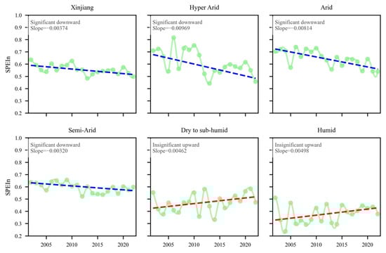
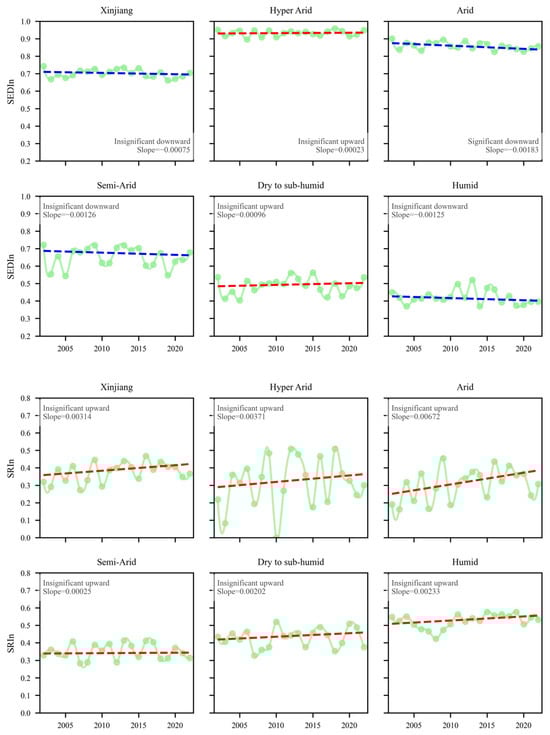
Figure 5.
Time trends of SPEIn-SSI, SEDIn-SSI and SRIn-SSI. The green line represents the change of the annual average, and the blue and red lines represent the downward and upward trend lines, respectively.
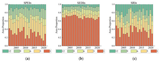
Figure 6.
Changes in area share by time scale for SPEIn (a), SEDIn (b) and SRIn (c).
4.3. Comparison of the Ability of Different Composite Indices to Recognize Ecological Drought
In this paper, abnormal changes in water deficit and soil moisture were considered important factors controlling ecological drought. Using the Copula method (P-MCDI) and the nonparametric method (NP-MCDI), and set up the composite index without considering the previous drought cumulative group of MCDIo and with the consideration of the previous drought cumulative group of MCDIs, the two scenarios, respectively, with the Section 4.1 obtained by calculating the SMn Pearson correlation (Figure 7). The average correlation values for P-MCDIo, P-MCDIs, NP-MCDIo and NP-MCDIs for the four scenarios were 0.57, 0.66, 0.54 and 0.66, respectively (Figure 5). Based on the mean values of the composite indices across the four cases, correlations were stronger when cumulative drought effects were considered. Under the same cumulative conditions, however, the two methods performed almost equally, indicating little difference between the indices obtained by the two methods.
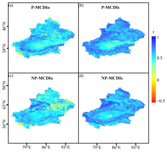
Figure 7.
Correlation between P-MCDIo (a), P-MCDIs (b), NP-MCDIo (c), NP-MCDIs (d), and SM.
Abnormal changes in the state of vegetation (NDVI) and GPP are important factors for ecological assessment. Excluding areas with mean values of NDVI lower than 0.1, the composite indices without considering the cumulative MCDIo of prior droughts and with considering the cumulative MCDIs of prior droughts were correlated with NDVI and GPP, respectively, using both the Copula method (P-MCDI) and the nonparametric method (NP-MCDI). Pearson correlations were calculated (Figure 8). For NDVI, the average correlations for P-MCDIo, P-MCDIs, NP-MCDIo and NP-MCDIs for the four cases were 0.23, 0.34, 026 and 0.38, respectively (Figure 9). For GPPs, the average correlations were 0.22, 0.31, 026 and 0.36, respectively (Figure 9). From the average correlation strengths of the four cases, the correlation was stronger for the same cumulative effect of considering the previous drought, while the correlation of the composite drought indices NP-MCDIs obtained by the nonparametric method was stronger for the same cumulative effect of drought. Considering NDVI, SMn and GPP, the differences between the two composite index methods were not significant. However, the nonparametric method performed better in capturing the dynamics of NDVI and GPP, suggesting that the composite indices NP-MCDIs are more effective overall.
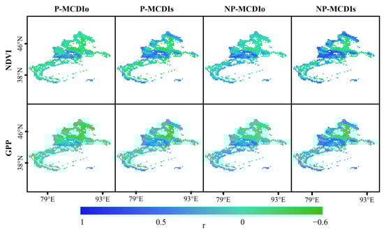
Figure 8.
Correlation between the four indices and NDVI and GPP.
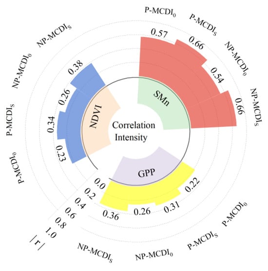
Figure 9.
Average correlation strength between the four indices and SM, NDVI, and GPP.
4.4. Validation of the Agricultural Drought Events
To further validate the applicability of the composite indices, drought classes assessed using P-MCDIs and NP-MCDIs (both considering the cumulative effect of previous droughts) were validated against actual drought events. The actual drought events in Xinjiang were queried from the China Drought and Water Hazard Bulletin from 2006 to 2022. Widespread summer droughts occurred in 2008, 2009, and 2022, and the applicability of the indices was analyzed by comparing the spatial distribution patterns of these recorded droughts with the two composite indices (Figure 10). Both indices used the same drought thresholds (Table 2). The results show that both indices successfully identified widespread summer droughts in all three years, with little difference in spatial patterns. To further evaluate potential differences, we calculated the hit rate of NP-MCDIs using the drought degree of P-MCDIs as the reference. The calculation rule was defined as follows: count plus 1 if the aridity is the same at the same location, +0.5 if the NP-MCDIs are more arid, and −0.5 if the NP-MCDIs are moister. The results show a hit rate of 100% in all three years. These results indicate that both indices are suitable for assessing ecological aridity when using the same threshold.
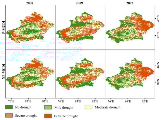
Figure 10.
Spatial distribution of P-MCDIs and NP-MCDIs during summer droughts.
4.5. Dominant Factors in Ecological Drought
In this study, ExtraTrees+SHAP was used to analyze the main drivers of integrated ecological drought. The average absolute SHAP values were applied to analyze the overall contribution of each factor during the study period (Figure 11). The factor with the largest absolute value per pixel was used as the dominant factor in order to analyze the spatial distribution pattern of dominant factors in Xinjiang (Figure 11a). It was found that SM was the dominant drought factor in 58.4% of the total area, widely distributed throughout Xinjiang. ED was dominant in 13.9% of the area, concentrated in the northern and northeastern part of Xinjiang. RF accounted for 9.5%, mainly concentrated in the southern region with low vegetation cover. Meteorological factors (WDs) were dominant in only 6.2% of the area, which was mainly distributed in the southwestern and northern part of Xinjiang. Based on mean absolute SHAP values (Figure 11b), the main factor contributing to ecological drought in Xinjiang was soil moisture (0.25), followed by ED (0.14) and RF (0.12). In contrast, the average contributions of water deficit (WD) and rainfall (PRE) were lower, at 0.07 and 0.05, respectively, suggesting that meteorological drought contributed less to ecological drought formation compared with SM, ED and RF.
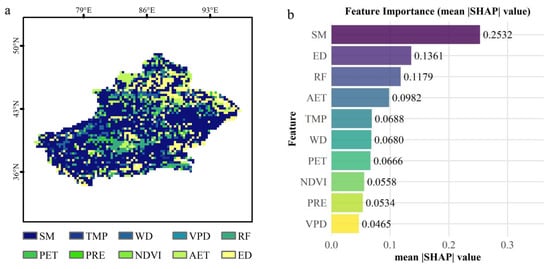
Figure 11.
The spatial distribution of the main driving factors of ecological drought (a) and the average SHAP value ranking (b).
We further examined the roles of SM, ED and RF in integrated ecological drought by analyzing their spatial distribution patterns and differences across climate scenarios (Figure 12). Regions where the effect of SM exceeded 0.3 were mainly distributed in the fringe zones of Xinjiang and the western region, which correspond primary to dry semi-humid and humid climates (Figure 12d). Meanwhile, the overall impact of SM decreased gradually from semi-arid to extra-arid regions. For ED, the impact exceeded 0.2 only in areas extending from the northeast to the southern edge, while the average impact across different climate regions remained below 0.2 (Figure 12e). For RF, impacts exceeded 0.3 only in the western and marginal regions, with average values below 0.2 across different climate regions (Figure 12f). The anomalously high average impact of RF in exceptionally dry climatic regions, compared with arid and semi-arid climatic regions, may be attributed to extremely water-scarce areas where short-duration heavy rainfall events exert disproportionate influence.
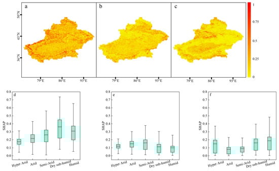
Figure 12.
Contributions and ranges of variation in SM (a,d), ED (b,e), and RF (c,f) in different climate regions.
4.6. Trends in the Sensitivity of Dominant Factors
To analyze the sensitivity of soil moisture (SM), evaporative demand (ED), and rainfall (RF), the slopes of SHAP values were calculated using the Theil–Sen estimator, with slope significance (p < 0.05) assessed by the Mann–Kendall test. Overall sensitivity during the study period was computed and grouped by SM level (Figure 13a,c,e), using a unified classification where regions with mean SM < 0.2 m3/m3 were designated as Arid and others as Humid. The analysis revealed intensified sensitivity to SM, ED, and RF with decreasing SM in Arid regions, while Humid regions showed a slight sensitivity increase with rising SM. Mean sensitivity magnitudes were 11.09 (SM), 1.66 (ED), and 2.47 (RF). Compared with Humid regions, Arid regions showed sensitivities 2.57 times higher for SM, 14.02 times higher for ED, and 2.88 times higher for RF. Further temporal analysis using a 3-year moving window (Figure 13b,d,f) indicated an overall increasing trend for all three factors despite temporal fluctuations. Sensitivity rises were especially pronounced during 2011–2013 and 2020–2022 (Figure 6), which may be linked to severe drought events in those years [46].
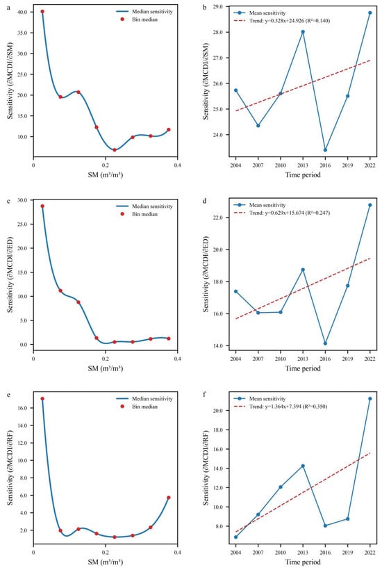
Figure 13.
Sensitivity and temporal trends in sensitivity of SM (a,b), ED (c,d), and RF (e,f) under different dry and wet conditions.
4.7. Driver Interaction Assessment
Further analysis examined interactive effects under dual-factor combinations (Figure 14). For Xinjiang as a whole, the SM-ED pairing exhibited the strongest negative feedback interaction, while ED-AET, SM-AET, and RF-PRE also showed pronounced negative feedback. Among positive feedback interactions, SM coupled with atmospheric variables (VPD, WD, TMP) showed the strongest effects. Drought-driving mechanisms varied across climatic zones. SM consistently played a central role in all regions, demonstrating peak interaction with ED (0.027 and 0.026) in Arid and Semi-Arid zones, respectively, while in Humid zones it showed peak interaction with RF (0.024). Moving from Hyper-Arid to Humid climates revealed systematic shifts in drought mechanisms: SM-ED interactions were dominated by negative feedback from Hyper-Arid to Semi-Arid zones but shifted to positive feedback in Dry Sub-Humid and Humid regions. SM-RF interactions maintained positive feedback across all zones but were significantly stronger in Humid regions. ED-AET displayed marked negative feedback in Hyper-Arid and Arid zones, transitioning to weak positive feedback in Humid regions, potentially because limited AET reductions in Arid zones paradoxically suppressed ED decrease. For RF, significant positive feedback with SM was observed only in Humid regions, while its interactions with other factors were generally negative.
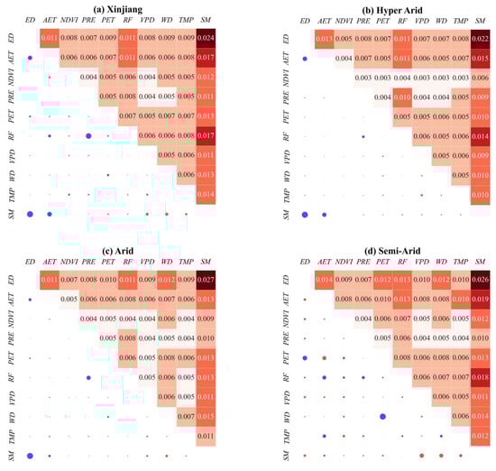
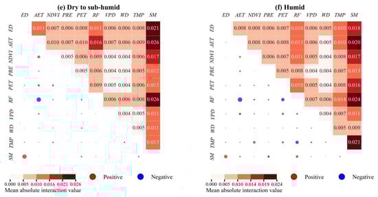
Figure 14.
Interaction between different factors.
5. Discussion
5.1. The Role of Cumulative Effects in Drought Propagation
As drought events continue to occur, the monitoring of combined droughts (agricultural/ecological droughts) is of great interest. Ecological drought is a process in which insufficient precipitation first affects soil, hydrology, vegetation and other systems, eventually developing into water stress across the entire ecosystem [5]. Atmospheric indicators such as precipitation (PRE), actual evapotranspiration (AET), and atmospheric evapotranspiration demand (AED) are commonly used in drought severity assessments. These metrics have been applied to measure atmospheric water deficit and generalized for multi-time scale droughts. measurements and predictions [61]. For example, SPI and SPEI can be adjusted for different time scales: short-term for meteorological drought, medium- and long-term for agricultural drought, and long-term for hydrological drought [32,62]. Based on these response relationships, the quantitative theory of drought cumulative effects has been proposed, in which the average cumulative period is determined by correlations between standardized indices and hydrometeorological factors, reflecting the propagation period between different drought types [34,38].
It is important to note that the drought accumulation period is not fixed. As shown in Figure 4, the accumulation period (time scale) of SPEI and SRI shows obvious fluctuations, likely due to uneven spatial and temporal distributions of rainfall and runoff, as well as interference from extreme rainfall. Spatially, SPEI is dominated by 1–3 months, suggesting that meteorological drought spreads to ecological drought at a faster rate. In addition, the correlation of SPEI during this transmission process showed a downward trend (Figure 5), and its contribution was low (Figure 11), indicating that the formation of ecological drought in Xinjiang is decoupling from WD, especially in arid climate regions (Figure 5). SEDI is spatially dominated by a 1-month scale, indicating that evapotranspiration deficit rapidly spreads to ecological drought. Although the correlation trend of SEDI during drought propagation is not obvious (Figure 5), its contribution is second only to soil moisture (Figure 11). This indicates that ecological drought in Xinjiang is closely related to ED, especially in arid climate regions, where ED and SM showed strong interactions (Figure 14). The spatial distribution of SRI is also dominated by a 1-month scale, suggesting that hydrological drought propagates rapidly to ecological drought. Although the correlation trend of SRI during drought propagation is not significantly increasing (Figure 5), its contribution remains relatively high (Figure 11). In addition, the sensitivity of ecological drought to RF showed the fastest growth rate (Figure 13), highlighting the increasing importance of RF in drought propagation. In general, ecological drought in Xinjiang is transmitted from evapotranspiration deficit (ED) to runoff deficit (RF), and eventually leads to ecological drought (SM anomaly). In addition, ecosystems exhibit a recovery period after drought, often requiring long time to fully recover [63]. Therefore, considering the cumulative effect of drought (propagation time) provides a scientific basis for drought management and ecological restoration.
5.2. The Role of Atmospheric Factors in Ecological Drought
As research has progressed, meteorological drought indicators such as SPEI have generated debate within the academic community. First, SPEI responds primarily to temporal changes in regional drought but does not adequately represent the relative severity of drought across space, and it performs poorly in some arid regions. For example, the use of SPEI in Northwest China (including Xinjiang) has shown poor performance [34,64]. Second, forecasts based on the Meteorological Drought Index (MDI) overestimate the severity of drought compared to the Drought Index (DI), which uses an ecological indicator. One reason is that AED tends to overestimate drought severity compared with AET, because actual evapotranspiration is constrained by water availability and by physiological and biophysical resistance, meaning AED does not reflect the true amount of evapotranspiration. Third, scholars continue to debate whether actual evapotranspiration (AET) or AED should be used in SPEI. Some argue that AET better represents the real water cycle, especially in water-limited areas [65] and note that SPEI ignores the complex relationship among AET, P and PET [66]. Other argue that AED has a unique response pattern: vegetation responds nonlinearly to high AED, first reducing transpiration to counteract atmospheric evapotranspiration pressure before the threshold is reached, and after the threshold is reached, plants accelerate transpiration to avoid death.
For the Xinjiang region, there are the following possible explanations. We found that the contribution of water deficit to ecological drought was very low, and the correlation between WD and soil moisture showed a decreasing trend. One hypothesis is that the weakened correlation between ecological drought and rainfall in Xinjiang arises from the uneven spatial and temporal distribution of rainfall. Related studies have shown that global vegetation responds more strongly to rainfall variability at daily or annual scales than to rainfall totals, suggesting that daily rainfall variability may be a major climatic driver of global changes in vegetation function [67]. Another possible explanation is that recharge from other water sources influences the land–air water cycle, such as increased runoff from glacier shrinkage [68].
Two key drivers are typically included in ecological and agricultural drought assessments: effective moisture and water demand [23]. Although many studies support the importance of soil moisture in compound drought (composite), soil moisture alone does not directly represent the water actually available for ecosystem use, whereas AET is a closer measure of effective water. At the same time, AED (denoted as PET in this paper) has a nonlinear response to vegetation indicators. Therefore, many studies support the use of SEDI, which combines AET and AED, as the best indicator for ecological and agricultural drought assessment [69,70].
In this study, the average correlation between SEDIn and SSI reached 0.72, indicating that SEDI is closely linked to soil moisture anomalies. We also observed that the average contribution of PRE was only 0.05, indicating that the role of rainfall is low in the formation of ecological drought. Independent contributions of AET (0.10) and PET (0.07) were lower than that of ED, suggesting that ED is more appropriate for the assessment of ecological drought. We also note that there is a nonlinear response relationship between ED and SM. For example, SM-ED interactions were dominated by positive feedback in Dry Sub-humid and Humid regions, where decreasing SM reduces AET flux to the atmosphere. At the same time, the surface temperature is less able to regulate, which in turn increases AED [71], ultimately manifesting itself as negative SM-ED feedback. A possible explanation for the dominance of negative feedback in Hyper-Arid to Semi-Arid regions is that as SM decreases, it regulates evapotranspiration and atmospheric moisture fluxes, thereby enhancing atmospheric moisture transport to arid regions [72].
5.3. Uncertainty in Vegetation Indicators
While there are more cases of vegetation indicators being used directly as ecological drought studies [73], there is some controversy over the response of vegetation change to climate and drought. Globally, a widespread greening trend has been observed [74]. Some argue that this greening trend may mask real droughts. For example, rainfall recovery after prolonged droughts and elevated CO2 may contribute to greening [74,75]. Elevated CO2 concentrations may also reduce the water requirements of vegetation photosynthesis, thereby increasing water-use efficiency [76]. In addition, its moderating effect on vegetation productivity becomes increasingly evident under scenario simulations with increasing CO2 [47]. While elevated CO2 levels promote plant growth and drought tolerance, increases in temperature and limitations in water availability still slow ecological recovery [77].
Others argue that greening trends may instead exacerbate aridity (atmospheric drought). Increased vegetation cover alters the atmospheric water cycle by increasing transpiration while reducing soil evaporation [78]. In semi-arid regions with strong coupling of aridity and vegetation, increased vegetation transpiration exacerbates soil aridity [79]. In addition, early greening due to warming has been linked to significant increases in evapotranspiration in late spring, persisting into summer and exacerbating hydrological drought in the Tianshan mountain watersheds of Xinjiang [80]. However, some researchers have pointed out that climate factors contribute more to ET variability than vegetation changes, since higher vegetation transpiration can be offset by reduced soil evaporation [81]. There are also differences across different climatic zones. In humid regions with dense (energy-limited) vegetation, warming-induced greening is limited, and increased vegetation can even reduce evapotranspiration by decreasing surface temperature. In arid regions with limited water resources, the pattern is reversed [82,83]. In addition, studies have shown that ecological restoration mitigates atmospheric drought through land-atmosphere coupling. For example, in arid regions of China, ecological restoration mitigated atmospheric drought in semi-arid zones by slowing down the increase in VPD. However, the opposite effect was observed in arid and semi-humid regions [84].
Overall, there remain many uncertainties in the applicability of vegetation metrics. First, measurement uncertainty of remote sensing information [85], especially in areas with low vegetation cover. Second, differences in vegetation response to drought across hydroclimatic zones, where applying uniform assessment criteria can introduce uncertainty in drought assessment [86]. Third, the influence of atmospheric CO2 concentrations on ecological and hydrological processes and physiological response of vegetation is highly uncertain [87,88,89]. Fourth, uncertainty in the assessment of vegetation trends by ESMs. For example, under the emergency constraint approach, ESMs may underestimate the greening trend and the associated future water scarcity [90].
6. Conclusions
In this study, we constructed a composite ecological drought index by incorporating the cumulative effects of drought using both Copula and nonparametric methods, integrating water deficit, soil moisture, evapotranspiration deficit, and runoff to examine differences in the two approaches. The main drivers and interactions of ecological drought in Xinjiang were analyzed using interpretable machine learning, and the spatial and temporal sensitivities of the three main factors—SM, ED, and RF—were also analyzed. The following conclusions were drawn from this study:
- (1)
- Of the two ED forms, EDr was superior to EDd in identifying soil moisture variability in the study area. The ED metrics performed better in the low VTA areas (sparsely vegetated).
- (2)
- For SPEI, SEDI, and SRI, cumulative effects on soil moisture variability were observed. For SPEI and SRI, the cumulative effect is dominated by short- and medium-term time scales in arid regions, while it is dominated by long-term time scales in humid regions. For SEDI, short-term time scales dominated overall.
- (3)
- A comprehensive ecological drought index was constructed using both Copula and nonparametric methods. Indices that considered cumulative effects performed better in capturing SM, NDVI, and GPP variability than those without cumulative effects. Meanwhile, we found that the performance of the composite index constructed by the nonparametric method was better than the composite index constructed by the Copula. However, in terms of drought degree classification, the two methods showed little difference. Therefore, the nonparametric method is recommended for producing global composite drought index datasets, as it improves computational efficiency compared with the Copula method, which requires numerous parameter assumptions.
- (4)
- By analyzing the influencing factors of the composite ecological drought index, it was found that SM anomaly was the main contributor to ecological drought, followed by ED and RF. Meanwhile, the interaction between ED and SM represented the strongest negative feedback in Xinjiang, indicating that their combined effect contributed the most to ecological drought.
- (5)
- The sensitivity of ecological drought to SM, ED, and RF increased nonlinearly with SM in the dry zone (SM below 0.2 m3/m3). In addition, sensitivities to all three factors fluctuated over time and showed abnormal increases during drought years.
In order to effectively assess ecological drought in Xinjiang, it is crucial to select appropriate indicators and methods. Based on the interactions among ecological elements in ecological drought, distinctive water resource management strategies should be designed for different climatic zones to enhance ecological drought resilience.
Author Contributions
H.T. (Hao Tang): Writing—original draft, Methodology. Q.L.: Writing—review and editing, Funding acquisition. H.T. (Hongfei Tao): Writing—review and editing. P.J.: Writing—review and editing. C.T.: Formal analysis. X.K.: Formal analysis. All authors have read and agreed to the published version of the manuscript.
Funding
Xinjiang Uygur Autonomous Region Major Science and Technology Special Project (2023A02002-1), Xinjiang Uygur Autonomous Region Natural Science Foundation Youth Science Fund Project (2022D01B86).
Institutional Review Board Statement
Not applicable.
Data Availability Statement
The original data presented in the study are openly available in MSWEP at https://www.gloh2o.org/mswep/#faq (accessed on 1 March 2024), GLEAM at https://www.gleam.eu/ (accessed on 4 August 2024), ERA5-land at https://cds.climate.copernicus.eu/ (accessed on 10 April 2024), National Earth System Science Data Center at https://www.geodata.cn/, and GOSIF GPP at https://globalecology.unh.edu/data/GOSIF-GPP.html (accessed on 26 April 2024).
Conflicts of Interest
The authors declare no conflicts of interest.
References
- Pradhan, P.; Costa, L.; Rybski, D.; Lucht, W.; Kropp, J.P. A systematic study of sustainable development goal (SDG) interactions. Earth’s Future 2017, 5, 1169–1179. [Google Scholar] [CrossRef]
- Guo, H.; Chen, J.; Pan, C. Assessment on agricultural drought vulnerability and spatial heterogeneity study in China. Int. J. Environ. Res. Public Health 2021, 18, 4449. [Google Scholar] [CrossRef]
- Li, Z.; Mu, Z.; Qiu, X.; Liu, J. Changes in future drought characteristics in the Ili River Basin, China, using the new comprehensive standardized drought index. Ecol. Indic. 2025, 173, 113412. [Google Scholar] [CrossRef]
- Zhang, Y.; Huang, S.; Huang, Q.; Leng, G.; Wang, H.; Wang, L. Assessment of drought evolution characteristics based on a nonparametric and trivariate integrated drought index. J. Hydrol. 2019, 579, 124230. [Google Scholar] [CrossRef]
- Zhao, Q.; Zhang, X.; Li, C.; Xu, Y.; Fei, J. Compound ecological drought assessment of China using a Copula-based drought index. Ecol. Indic. 2024, 164, 112141. [Google Scholar] [CrossRef]
- Wang, F.; Lai, H.; Li, Y.; Feng, K.; Tian, Q.; Guo, W.; Zhang, W.; Di, D.; Yang, H. Dynamic variations of terrestrial ecological drought and propagation analysis with meteorological drought across the mainland China. Sci. Total Environ. 2023, 896, 165314. [Google Scholar] [CrossRef]
- Jiang, T.; Su, X.; Zhang, G.; Zhang, T.; Wu, H. Estimating propagation probability from meteorological to ecological droughts using a hybrid machine learning copula method. Hydrol. Earth Syst. Sci. 2023, 27, 559–576. [Google Scholar] [CrossRef]
- Peterson, T.J.; Saft, M.; Peel, M.C.; John, A. Watersheds may not recover from drought. Science 2021, 372, 745–749. [Google Scholar] [CrossRef]
- Chen, S.; Yuan, X. The timing of detectable increases in seasonal soil moisture droughts under future climate change. Earth’s Future 2024, 12, e2023EF004174. [Google Scholar] [CrossRef]
- Cui, J.; Chen, A.; Huntingford, C.; Piao, S. Integrating ecosystem water demands into drought monitoring and assessment under climate change. Nat. Water 2024, 2, 215–218. [Google Scholar] [CrossRef]
- Zhang, Y.; Hao, Z.; Jiang, Y.; Singh, V.P. Impact-based evaluation of multivariate drought indicators for drought monitoring in China. Glob. Planet. Change 2023, 228, 104219. [Google Scholar] [CrossRef]
- da Silva, G.J.F.; Silva, R.M.D.; Brasil Neto, R.M.; Silva, J.F.C.B.C.; Dantas, A.P.X.; Santos, C.A.G. Multi-datasets to monitor and assess meteorological and hydrological droughts in a typical basin of the Brazilian semiarid region. Environ. Monit. Assess. 2024, 196, 368. [Google Scholar] [CrossRef]
- Tian, Q.; Wang, F.; Tian, Y.; Jiang, Y.; Weng, P.; Li, J. Copula-based comprehensive drought identification and evaluation over the Xijiang River Basin in South China. Ecol. Indic. 2023, 154, 110503. [Google Scholar] [CrossRef]
- Wang, F.; Wang, Z.; Yang, H.; Di, D.; Zhao, Y.; Liang, Q. A new copula-based standardized precipitation evapotranspiration streamflow index for drought monitoring. J. Hydrol. 2020, 585, 124793. [Google Scholar] [CrossRef]
- Guo, W.; Huang, S.; Huang, Q.; She, D.; Shi, H.; Leng, G.; Li, J.; Cheng, L.; Gao, Y.; Peng, J. Precipitation and vegetation transpiration variations dominate the dynamics of agricultural drought characteristics in China. Sci. Total Environ. 2023, 898, 165480. [Google Scholar] [CrossRef]
- Yang, C.; Liu, C.; Gu, Y.; Wang, Y.; Xing, X.; Ma, X. A novel comprehensive agricultural drought index accounting for precipitation, evapotranspiration, and soil moisture. Ecol. Indic. 2023, 154, 110593. [Google Scholar] [CrossRef]
- Zhang, Q.; Shi, R.; Xu, C.-Y.; Sun, P.; Yu, H.; Zhao, J. Multisource data-based integrated drought monitoring index: Model development and application. J. Hydrol. 2022, 615, 128644. [Google Scholar] [CrossRef]
- Li, L.; She, D.; Zheng, H.; Lin, P.; Yang, Z.-L. Elucidating diverse drought characteristics from two meteorological drought indices (SPI and SPEI) in China. J. Hydrometeorol. 2020, 21, 1513–1530. [Google Scholar] [CrossRef]
- Wang, W.; Yang, H.; Huang, S.; Wang, Z.; Liang, Q.; Chen, S. Trivariate copula functions for constructing a comprehensive atmosphere-land surface-hydrology drought index: A case study in the Yellow River basin. J. Hydrol. 2024, 642, 131784. [Google Scholar] [CrossRef]
- Suo, N.; Xu, C.; Cao, L.; Song, L.; Lei, X. A copula-based parametric composite drought index for drought monitoring and applicability in arid Central Asia. Catena 2024, 235, 107624. [Google Scholar] [CrossRef]
- Xu, L.; Chen, N.; Yang, C.; Zhang, C.; Yu, H. A parametric multivariate drought index for drought monitoring and assessment under climate change. Agric. For. Meteorol. 2021, 310, 108657. [Google Scholar] [CrossRef]
- Liu, Y.; Yu, X.; Dang, C.; Yue, H.; Wang, X.; Niu, H.; Zu, P.; Cao, M. A dryness index TSWDI based on land surface temperature, sun-induced chlorophyll fluorescence, and water balance. ISPRS J. Photogramm. Remote Sens. 2023, 202, 581–598. [Google Scholar] [CrossRef]
- Vicente-Serrano, S.M.; Domínguez-Castro, F.; Beguería, S.; El Kenawy, A.; Gimeno-Sotelo, L.; Franquesa, M.; Azorin-Molina, C.; Andres-Martin, M.; Halifa-Marín, A. Atmospheric drought indices in future projections. Nat. Water 2025, 3, 374–387. [Google Scholar] [CrossRef]
- Otkin, J.A.; Anderson, M.C.; Hain, C.; Mladenova, I.E.; Basara, J.B.; Svoboda, M. Examining rapid onset drought development using the thermal infrared–based evaporative stress index. J. Hydrometeorol. 2013, 14, 1057–1074. [Google Scholar] [CrossRef]
- Chang, Q.; Ficklin, D.L.; Jiao, W.; Denham, S.O.; Wood, J.D.; Brunsell, N.A.; Matamala, R.; Cook, D.R.; Wang, L.; Novick, K.A. Earlier ecological drought detection by involving the interaction of phenology and eco-physiological function. Earth’s Future 2023, 11, e2022EF002667. [Google Scholar] [CrossRef]
- Miralles, D.; Gentine, P.; Seneviratne, S.I.; Teuling, A. Land-atmospheric feedbacks during droughts and heatwaves: State of the science and current challenges. Ann. N. Y. Acad. Sci. 2018, 1436, 19–35. [Google Scholar] [CrossRef]
- Seneviratne, S.I.; Corti, T.; Davin, E.L.; Hirschi, M.; Jaeger, E.B.; Lehner, I.; Orlowsky, B.; Teuling, A.J. Investigating soil moisture–climate interactions in a changing climate: A review. Earth-Sci. Rev. 2010, 99, 125–161. [Google Scholar] [CrossRef]
- Konapala, G.; Mishra, A.K.; Wada, Y. Climate change will affect global water availability through compounding changes in seasonal precipitation and evaporation. Nat. Commun. 2020, 11, 3044. [Google Scholar] [CrossRef]
- Hobbins, M.T.; Wood, A.; McEvoy, D.J.; Huntington, J.L.; Morton, C.; Anderson, M.; Hain, C. The evaporative demand drought index. Part I: Linking drought evolution to variations in evaporative demand. J. Hydrometeorol. 2016, 17, 1745–1761. [Google Scholar] [CrossRef]
- Gumus, V. Evaluating the effect of the SPI and SPEI methods on drought monitoring over Turkey. J. Hydrol. 2023, 626, 130386. [Google Scholar] [CrossRef]
- Dikici, M.; Aksel, M. Comparison of SPI, SPEI and SRI drought indices for Seyhan Basin. Int. J. Electron. Mech. Mechatron. Eng. 2019, 9, 1751–1762. [Google Scholar]
- Potop, V.; Možný, M.; Soukup, J. Drought evolution at various time scales in the lowland regions and their impact on vegetable crops in the Czech Republic. Agric. For. Meteorol. 2012, 156, 121–133. [Google Scholar] [CrossRef]
- Li, J.; Wang, Z.; Wu, X.; Xu, C.-Y.; Guo, S.; Chen, X. Toward monitoring short-term droughts using a novel daily scale, standardized antecedent precipitation evapotranspiration index. J. Hydrometeorol. 2020, 21, 891–908. [Google Scholar] [CrossRef]
- Lu, Y.; Yang, T.; Fu, J.; Song, W. Utility of the standardized precipitation evapotranspiration index (SPEI) to detect agricultural droughts over China. J. Hydrol. Reg. Stud. 2025, 58, 102190. [Google Scholar] [CrossRef]
- Sun, P.; Liu, R.; Yao, R.; Shen, H.; Bian, Y. Responses of agricultural drought to meteorological drought under different climatic zones and vegetation types. J. Hydrol. 2023, 619, 129305. [Google Scholar] [CrossRef]
- Sosa, G.; Fernández-Long, M.E.; Vicente-Serrano, S.M. Evaluating the performance of drought indices for assessing agricultural droughts in Argentina. Agron. J. 2025, 17, e70008. [Google Scholar] [CrossRef]
- Javed, T.; Li, Y.; Rashid, S.; Li, F.; Hu, Q.; Feng, H.; Chen, X.; Ahmad, S.; Liu, F.; Pulatov, B. Performance and relationship of four different agricultural drought indices for drought monitoring in China’s mainland using remote sensing data. Sci. Total Environ. 2021, 759, 143530. [Google Scholar] [CrossRef] [PubMed]
- Yuan, M.; Gan, G.; Bu, J.; Su, Y.; Ma, H.; Liu, X.; Zhang, Y.; Gao, Y. A new multivariate composite drought index considering the lag time and the cumulative effects of drought. J. Hydrol. 2025, 653, 132757. [Google Scholar] [CrossRef]
- Zhu, J.; Zhou, L.; Huang, S. A hybrid drought index combining meteorological, hydrological, and agricultural information based on the entropy weight theory. Arab. J. Geosci. 2018, 11, 91. [Google Scholar] [CrossRef]
- Hosseini, Z.S.; Moghaddasi, M.; Palmozd, S. Simultaneous monitoring of different drought types using linear and nonlinear combination approaches. Water Resour. Manag. 2023, 37, 1125–1151. [Google Scholar] [CrossRef]
- Qing, Y.; Wang, S.; Ancell, B.C.; Yang, Z.L. Accelerating flash droughts induced by the joint influence of soil moisture depletion and atmospheric aridity. Nat. Commun. 2022, 13, 1139. [Google Scholar] [CrossRef] [PubMed]
- Krich, C.; Mahecha, M.D.; Migliavacca, M.; De Kauwe, M.G.; Griebel, A.; Runge, J.; Miralles, D.G. Decoupling between ecosystem photosynthesis and transpiration: A last resort against overheating. Environ. Res. Lett. 2022, 17, 044013. [Google Scholar] [CrossRef]
- Hao, Z.; AghaKouchak, A. Multivariate Standardized Drought Index: A parametric multi-index model. Adv. Water Resour. 2013, 57, 12–18. [Google Scholar] [CrossRef]
- Vicente-Serrano, S.M.; Beguería, S.; López-Moreno, J.I. A multiscalar drought index sensitive to global warming: The standardized precipitation evapotranspiration index. J. Clim. 2010, 23, 1696–1718. [Google Scholar] [CrossRef]
- Gebrechorkos, S.H.; Sheffield, J.; Vicente-Serrano, S.M.; Funk, C.; Miralles, D.G.; Peng, J.; Dyer, E.; Talib, J.; Beck, H.E.; Singer, M.B.; et al. Warming accelerates global drought severity. Nature 2025, 642, 628–635. [Google Scholar] [CrossRef]
- Liu, M.; Trugman, A.T.; Peñuelas, J.; Anderegg, W.R.L. Climate-driven disturbances amplify forest drought sensitivity. Nat. Clim. Change 2024, 14, 746–752. [Google Scholar] [CrossRef]
- Qi, G.; Song, J.; Chen, S.; Gong, Y.; Bai, H.; She, D.; Xia, J.; Fu, Y.H. Increasing impacts of compound extreme droughts on vegetation productivity in China. J. Hydrol. 2025, 660, 133447. [Google Scholar] [CrossRef]
- Li, W.; Migliavacca, M.; Forkel, M.; Walther, S.; Reichstein, M.; Orth, R. Widespread increasing vegetation sensitivity to soil moisture. Nat. Commun. 2022, 13, 3959. [Google Scholar] [CrossRef]
- Li, Y.-X.; Leng, P.; Kasim, A.A.; Li, Z.-L. Spatiotemporal variability and dominant driving factors of satellite observed global soil moisture from 2001 to 2020. J. Hydrol. 2025, 654, 132848. [Google Scholar] [CrossRef]
- Yu, J.; Wang, W.; Chen, Z.; Cao, M.; Qian, H. Disentangling the dominance of atmospheric and soil water stress on vegetation productivity in global drylands. J. Hydrol. 2025, 657, 133043. [Google Scholar] [CrossRef]
- Yu, X.; Zhang, Q.; Zeng, X.; Dai, S. The distribution and driving climatic factors of agricultural drought in China: Past and future perspectives. J. Environ. Manag. 2025, 377, 124599. [Google Scholar] [CrossRef]
- Wu, X.; Zhang, C.; Dong, S.; Hu, J.; Tong, X.; Zheng, X. Spatiotemporal changes of the aridity index in Xinjiang over the past 60 years. Environ. Earth Sci. 2023, 82, 392. [Google Scholar] [CrossRef]
- Zhang, Y.; Long, A.; Lv, T.; Deng, X.; Wang, Y.; Pang, N.; Lai, X.; Gu, X. Trends, cycles, and spatial distribution of the precipitation, potential evapotranspiration, and aridity index in Xinjiang, China. Water 2022, 15, 62. [Google Scholar] [CrossRef]
- Zhang, X.; Wang, X.; Zhou, B. CMIP6-projected changes in drought over Xinjiang, Northwest China. Int. J. Climatol. 2023, 43, 6560–6577. [Google Scholar] [CrossRef]
- Roderick, M.L.; Greve, P.; Farquhar, G.D. On the assessment of aridity with changes in atmospheric CO2. Water Resour. Res. 2015, 51, 5450–5463. [Google Scholar] [CrossRef]
- Feng, T.; Su, T.; Ji, F.; Zhi, R.; Han, Z. Temporal characteristics of actual evapotranspiration over China under global warming. J. Geophys. Res. Atmos. 2018, 123, 5845–5858. [Google Scholar] [CrossRef]
- Zomer, R.J.; Xu, J.; Trabucco, A. Version 3 of the global aridity index and potential evapotranspiration database. Sci. Data 2022, 9, 409. [Google Scholar] [CrossRef] [PubMed]
- Barrow, C.J. World atlas of desertification (United nations environment programme). Land Degrad. Dev. 1992, 3, 249. [Google Scholar] [CrossRef]
- Lavagnini, I.; Badocco, D.; Pastore, P.; Magno, F. Theil–Sen nonparametric regression technique on univariate calibration, inverse regression and detection limits. Talanta 2011, 87, 180–188. [Google Scholar] [CrossRef]
- Guo, M.; Li, J.; He, H.S.; Xu, J.; You-hai, J. Detecting global vegetation changes using Mann-Kendal (MK) trend test for 1982–2015 time period. Chin. Geogr. Sci. 2018, 28, 907–919. [Google Scholar] [CrossRef]
- Mohammed, S.; Arshad, S.; Alsilibe, F.; Ul Moazzam, M.F.; Bashir, B.; Prodhan, F.A.; Alsalman, A.; Vad, A.; Ratonyi, T.; Harsányi, E. Utilizing machine learning and CMIP6 projections for short-term agricultural drought monitoring in central Europe (1900–2100). J. Hydrol. 2024, 633, 130968. [Google Scholar] [CrossRef]
- Tirivarombo, S.O.D.E.; Osupile, D.; Eliasson, P. Drought monitoring and analysis: Standardised precipitation evapotranspiration index (SPEI) and standardised precipitation index (SPI). Phys. Chem. Earth Parts A/B/C 2018, 106, 1–10. [Google Scholar] [CrossRef]
- Boulton, C.A.; Lenton, T.M.; Boers, N. Pronounced loss of Amazon rainforest resilience since the early 2000s. Nat. Clim. Change 2022, 12, 271–278. [Google Scholar] [CrossRef]
- Bai, H.; Hua, B. Copula-based standardized precipitation evapotranspiration index and its evaluation in China. J. Hydrol. 2022, 615, 128587. [Google Scholar] [CrossRef]
- Rehana, S.; Monish, N.T. Characterization of regional drought over water and energy limited zones of India using potential and actual evapotranspiration. Earth Space Sci. 2020, 7, e2020EA001264. [Google Scholar] [CrossRef]
- Abiodun, B.J.; Makhanya, N.; Petja, B.M.; Abatan, A.A.; Oguntunde, P.G. Future projection of droughts over major river basins in Southern Africa at specific global warming levels. Theor. Appl. Climatol. 2018, 137, 1785–1799. [Google Scholar] [CrossRef]
- Feldman, A.F.; Konings, A.G.; Gentine, P.; Cattry, M.; Wang, L.; Smith, W.K.; Biederman, J.A.; Chatterjee, A.; Joiner, J.; Poulter, B. Large global-scale vegetation sensitivity to daily rainfall variability. Nature 2024, 636, 380–384. [Google Scholar] [CrossRef]
- Yao, J.; Chen, Y.; Guan, X.; Zhao, Y.; Chen, J.; Mao, W. Recent climate and hydrological changes in a mountain–basin system in Xinjiang, China. Earth-Sci. Rev. 2022, 226, 103957. [Google Scholar] [CrossRef]
- Yang, Y.; Anderson, M.C.; Gao, F.; Wardlow, B.; Hain, C.R.; Otkin, J.A.; Alfieri, J.; Yang, Y.; Sun, L.; Dulaney, W. Field-scale mapping of evaporative stress indicators of crop yield: An application over Mead, NE, USA. Remote Sens. Environ. 2018, 210, 387–402. [Google Scholar] [CrossRef]
- Nguyen, H.; Wheeler, M.C.; Otkin, J.A.; Cowan, T.; Frost, A.; Stone, R. Using the evaporative stress index to monitor flash drought in Australia. Environ. Res. Lett. 2019, 14, 064016. [Google Scholar] [CrossRef]
- Christian, J.I.; Basara, J.B.; Hunt, E.D.; Otkin, J.A.; Furtado, J.C.; Mishra, V.; Xiao, X.; Randall, R.M. Global distribution, trends, and drivers of flash drought occurrence. Nat. Commun. 2021, 12, 6330. [Google Scholar] [CrossRef]
- Zhou, S.; Williams, A.P.; Lintner, B.R.; Berg, A.M.; Zhang, Y.; Keenan, T.F.; Cook, B.I.; Hagemann, S.; Seneviratne, S.I.; Gentine, P. Soil moisture–atmosphere feedbacks mitigate declining water availability in drylands. Nat. Clim. Change 2021, 11, 38–44. [Google Scholar] [CrossRef]
- Wang, Y.; Liu, T.; Duan, L.; Chu, S.; Sun, J.; Tong, X.; Hao, L.; Bao, Y.; Gong, Y. A novel index combining meteorological, hydrological, and ecological anomalies used for ecological drought assessment at a grassland-type basin scale. Ecol. Indic. 2025, 173, 113384. [Google Scholar] [CrossRef]
- Zhu, Z.; Piao, S.; Myneni, R.B.; Huang, M.; Zeng, Z.; Canadell, J.G.; Ciais, P.; Sitch, S.; Friedlingstein, P.; Arneth, A.; et al. Greening of the Earth and its drivers. Nat. Clim. Change 2016, 6, 791–795. [Google Scholar] [CrossRef]
- Horion, S.; Swinnen, E. Assessing land degradation/recovery in the African Sahel from long-term earth observation based primary productivity and precipitation relationships. Remote Sens. 2013, 5, 664–686. [Google Scholar] [CrossRef]
- Ainsworth, E.A.; Rogers, A. The response of photosynthesis and stomatal conductance to rising [CO2]: Mechanisms and environmental interactions. Plant Cell Environ. 2007, 30, 258–270. [Google Scholar] [CrossRef]
- Belagam, V.; Sharma, A. Increasing cumulative impacts of droughts under climate change does not alter the ecosystem resilience in India. Earth’s Future 2025, 13, e2024EF005888. [Google Scholar] [CrossRef]
- Sun, S.; Bi, Z.; Mu, M.; Liu, Y.; Zhang, Y.; Li, J.; Liu, Y.; Zhou, Y.; Zhou, B.; Chen, H. Quantifying impacts of vegetation greenness change on drought over global vegetation zones. Geophys. Res. Lett. 2025, 52, e2024GL111634. [Google Scholar] [CrossRef]
- Yang, H.; Ma, F.; Yuan, X.; Ji, P.; Li, C. Vegetation greening accelerated the propagation from meteorological to soil droughts in the Loess Plateau from a three-dimensional perspective. J. Hydrol. 2025, 650, 132522. [Google Scholar] [CrossRef]
- Zheng, L.; Chen, R.; Xu, J.; Li, Y.; Jia, N.; Guo, X. Earlier vegetation green-up is intensifying hydrological drought in the Tianshan Mountain basins. J. Hydrol. Reg. Stud. 2025, 59, 102321. [Google Scholar] [CrossRef]
- Luo, Y.; Ma, N.; Zhang, Y. Divergent vegetation greening’s direct impacts on land-atmosphere water and carbon exchanges in the northeastern Tibetan Plateau. Glob. Planet. Change 2025, 251, 104825. [Google Scholar] [CrossRef]
- Chen, S.; Yuan, X.; Ji, P.; Yuan, S.; Lu, C. Direct vegetation response to CO2 rise is critical in projecting seasonal soil moisture droughts in mainland China. J. Hydrol. 2025, 661, 133639. [Google Scholar] [CrossRef]
- Luan, J.; Ma, N. Responses of seasonal hydrological processes to vegetation change in the Yellow River basin. J. Hydrol. 2025, 660, 133449. [Google Scholar] [CrossRef]
- Zhang, Y.; Feng, X.; Zhou, C.; Sun, C.; Leng, X.; Fu, B. Aridity threshold of ecological restoration mitigated atmospheric drought via land-atmosphere coupling in drylands. Commun. Earth Environ. 2024, 5, 381. [Google Scholar] [CrossRef]
- Yang, B.; Cui, Q.; Meng, Y.; Zhang, Z.; Hong, Z.; Hu, F.; Li, J.; Tao, C.; Wang, Z.; Zhang, W. Combined multivariate drought index for drought assessment in China from 2003 to 2020. Agric. Water Manag. 2023, 281, 108241. [Google Scholar] [CrossRef]
- Zhang, X.; Zhang, B. The responses of natural vegetation dynamics to drought during the growing season across China. J. Hydrol. 2019, 574, 706–714. [Google Scholar] [CrossRef]
- De Kauwe, M.G.; Medlyn, B.E.; Tissue, D.T. To what extent can rising [CO2] ameliorate plant drought stress? New Phytol. 2021, 231, 2118–2124. [Google Scholar] [CrossRef] [PubMed]
- Vicente-Serrano, S.M.; Miralles, D.G.; McDowell, N.; Brodribb, T.; Domínguez-Castro, F.; Leung, R.; Koppa, A. The uncertain role of rising atmospheric CO2 on global plant transpiration. Earth-Sci. Rev. 2022, 230, 104055. [Google Scholar] [CrossRef]
- Lesk, C.S.; Winter, J.M.; Mankin, J.S. Projected runoff declines from plant physiological effects on precipitation. Nat. Water 2025, 3, 167–177. [Google Scholar] [CrossRef]
- Chai, Y.; Miao, C.; Slater, L.; Ciais, P.; Berghuijs, W.R.; Chen, T.; Huntingford, C. Underestimating global land greening: Future vegetation changes and their impacts on terrestrial water loss. One Earth 2025, 8, 101176. [Google Scholar] [CrossRef]
Disclaimer/Publisher’s Note: The statements, opinions and data contained in all publications are solely those of the individual author(s) and contributor(s) and not of MDPI and/or the editor(s). MDPI and/or the editor(s) disclaim responsibility for any injury to people or property resulting from any ideas, methods, instructions or products referred to in the content. |
© 2025 by the authors. Licensee MDPI, Basel, Switzerland. This article is an open access article distributed under the terms and conditions of the Creative Commons Attribution (CC BY) license (https://creativecommons.org/licenses/by/4.0/).