Article

Smart Detection of Tomato Leaf Diseases Using Transfer Learning-Based Convolutional Neural Networks

1
Agricultural Engineering Department, Ain Shams University, Cairo 11221, Egypt
2
Department of Horticulture, College of Agricultural & Life Sciences, University of Wisconsin-Madison, Madison, WI 53705, USA
*
Author to whom correspondence should be addressed.
Agriculture 2023, 13(1), 139; https://doi.org/10.3390/agriculture13010139
Submission received: 8 December 2022 / Revised: 26 December 2022 / Accepted: 3 January 2023 / Published: 5 January 2023
(This article belongs to the Section Agricultural Technology)

Abstract

:
Plant diseases affect the availability and safety of plants for human and animal consumption and threaten food safety, thus reducing food availability and access, as well as reducing crop yield and quality. There is a need for novel disease detection methods that can be used to reduce plant losses due to disease. Thus, this study aims to diagnose tomato leaf diseases by classifying healthy and unhealthy tomato leaf images using two pre-trained convolutional neural networks (CNNs): Inception V3 and Inception ResNet V2. The two models were trained using an open-source database (PlantVillage) and field-recorded images with a total of 5225 images. The models were investigated with dropout rates of 5%, 10%, 15%, 20%, 25%, 30%, 40%, and 50%. The most important results showed that the Inception V3 model with a 50% dropout rate and the Inception ResNet V2 model with a 15% dropout rate, as they gave the best performance with an accuracy of 99.22% and a loss of 0.03. The high-performance rate shows the possibility of utilizing CNNs models for diagnosing tomato diseases under field and laboratory conditions. It is also an approach that can be expanded to support an integrated system for diagnosing various plant diseases.

1. Introduction

Tomatoes (Solanum lycopersium L.) are one of the world’s most widely produced and consumed vegetables. Tomato disease management is a necessary process that limits the improvement in crop quality and growth and represents a large part of the total production costs [1]. Therefore, accurate and rapid diagnosis of diseases is vital to reduce processing costs, the environmental impact of chemicals, and the risk of crop loss. Plant diseases affect crops, ranging from the appearance of some mild symptoms to the complete destruction of crops. Advances in artificial intelligence, image processing, and the presence of databases with different images help in the easy diagnosis and classification of plant diseases [2,3]. This is typically accomplished using machine learning techniques, allowing machines to perform tasks by learning from available data rather than running a static computer program designed specifically for the situation at hand.
Artificial intelligence (AI) applications have made significant progress as a result of the development of graphics processing units (GPUs), especially in machine learning applications. Several studies [4,5] employed conventional machine vision algorithms for disease identification, which may pinpoint the sites of pests and diseases as well as the extent of disease transmission. One of the uses of conventional machine learning is to identify objects in images. These applications use deep learning technology classes [6]. Deep learning applications for vision tasks go back to convolutional networks in the early 1990s. It is making significant advances in solving problems that have resisted the best efforts of the AI community for many years. The deep learning method includes the main benefits of current traditional image processing methods of taking advantage of the feature hierarchy and using architecture optimization to define processes such as feature extraction, selection, and classification [7].
Convolutional Neural Networks (CNNs) are deep learning algorithms with local connection and weight-sharing characteristics [8]. In recent years, numerous industries have experienced the successful implementation of CNN. The use of computer vision in precision agriculture has also grown due to CNNs’ remarkable performance as they have proven to be a good alternative for identifying plant diseases. CNN is a typical architecture that has lately been used to manage several machine learning tasks [9] and it is a type of neural network that uses deep learning to operate [10]. Input layers, convolution layers, pooling layers, and fully connected layers are all common components of a CNN architecture [6]. Face recognition, language processing, age prediction, time series classification, plant disease diagnosis, and other image analysis domains have successfully used the CNN architecture [11,12,13,14].
Plant diseases have traditionally been diagnosed through visual examination of leaf symptoms or through chemical examination, which are more time-consuming and costly methods. Moreover, some techniques have been used to diagnose diseases, such as machine learning techniques, expert systems, and others [15,16]. Traditional machine learning techniques, such as support vector machine (SVM), random forest (RF), and decision tree (DT) are limited in processing data in raw form. These algorithms have simple rules, a single structure, and fine classification performance in particular cases but require the manual construction of corresponding features derived from specific prior knowledge to train the model. Deep learning is better than traditional machine learning methods as it extracts deep features that are more accurate than traditional features in highlighting morphological differences from images [17]. One of the drawbacks of expert systems methods is their reliance on prior human knowledge to identify diseases. Therefore, deep learning methods that extract features are used to diagnose diseases [18].
Deep learning techniques have been used in various agricultural applications, in-cluding the classification of different types of crops [13], recognizing plant parts to locate harvesting sites by harvesting robots [14], and crop water stress monitoring [19]. Likewise, some authors have carried out research on diagnosing plant diseases by CNN methods [20,21,22,23,24,25,26]. Mohanty et al. [2] diagnosed diseases for 14 crop species and 26 diseases in the PlantVillage open dataset using pre-trained deep learning models and the greatest categorization accuracy was 99.35%. Chen et al. [27] developed VGGNet to train about 1000 images of five rice diseases and four maize diseases using general data and data collected for rice diseases. Fan et al. [28] improved the Inception V3 network for the identification of apple and coffee leaf diseases by integrating the features extracted by transfer learning with the features extracted by traditional methods. Yu et al. [29] used a deep learning model to diagnose tomato pests. Moreover, Karthik et al. [30] used the CNN model to identify the infection type in tomato leaf tissue and Abbas et al. [21] trained a deep learning network to diagnose tomato leaf diseases and the results were satisfactory. Moreover, CNN is a powerful tool for diagnosing plant diseases.
The training dataset is a key factor in how well CNN models perform. Despite good previous model results, these studies’ primary flaw was that the datasets were taken from an experimental (laboratory) environment, where machine perception conditions were relatively ideal. With the neglect of real field conditions. To the best of our knowledge, the application of CNN models in detecting tomato leaf diseases under field conditions has not been investigated. Therefore, the study aims to diagnose tomato leaf diseases by training a dataset collected under laboratory and field conditions to classify images of healthy and unhealthy tomato leaves using two pre-trained convolutional neural networks (CNNs) namely Inception V3 and Inception ResNet V2.

2. Materials and Methods

As shown in Figure 1, an overview of our method for identifying tomato leaf diseases is presented as follows: (a) dataset collection; (b) image pre-processing and augmentation; (c) learning phase; and (d) evaluation phase. Detailed descriptions of these stages are described in subsequent sections.

2.1. Dataset Collection

The dataset (images of tomato leaves) was obtained from two sources: (i) PlantVillage database (https://plantvillage.psu.edu/ (accessed on 20 September 2021)), which is an open and accessible database [31]. These data were used to diagnose plant diseases and were captured at experimental research stations associated with Land Grant Universities in the United States (Penn State, Florida, Cornell, and others). The database contains 54,305 images of infected and healthy leaves of 14 different crops, such as tomatoes, apples, and others. In this paper, only a set of tomato crop images were used. The set used includes three categories: two categories representing infected tomato leaves and a category representing healthy leaves as shown in Figure 2, and it consists of 3529 images; (ii) The image sets were captured from the field by a phone camera 24 megapixels. It contains 1696 images of the three categories: Early Blight, Yellow Leaf Curl Virus, and Healthy. The field dataset was photographed under normal field conditions between 7–10 AM at the farm of the Faculty of Agriculture, Ain Shams University, Egypt (30.112851 E, 31.243468 N) for the winter of 2021. The total dataset from the two sources in each category contains 5225 images of three different categories as shown in Table 1. The description of the diseases under study is described in Table 2.

2.2. Image Pre-Processing and Augmentation

In our experiments, image pre-processing, data augmentation, and CNN algorithms were implemented using Anaconda3 (Python 3.6), Keras-GPU library (KerasGPU). Available online: https://anaconda.org/anaconda/keras-gpu (accessed on 17 March 2022) and the experimental hardware environment includes a Windows 10 Pro workstation with an Intel Core i5-11400f CPU (16 GB of RAM) and a GeForce RTX 3060 Ti GPU (8 GB of memory) for CPU acceleration.
After field data were collected, they were categorized into three different categories (Early Blight, Yellow Leaf Curl Virus, and Health). Then, pre-processing was performed on the images using the Python programming language such as resizing and data augmentation. Images captured from the field have a size of 5632 × 4224 pixels, while the size of the botanical village data images is 256 × 256 pixels. All images are resized to 299 × 299 pixels when training the Inception V3 and Inception ResNet V2 models. After that, the images were shuffled every 42 images. Then, the images were divided into 80% training, 10% validation, and 10% testing. Each step contains a different number of batches, and each batch contains 32 images.
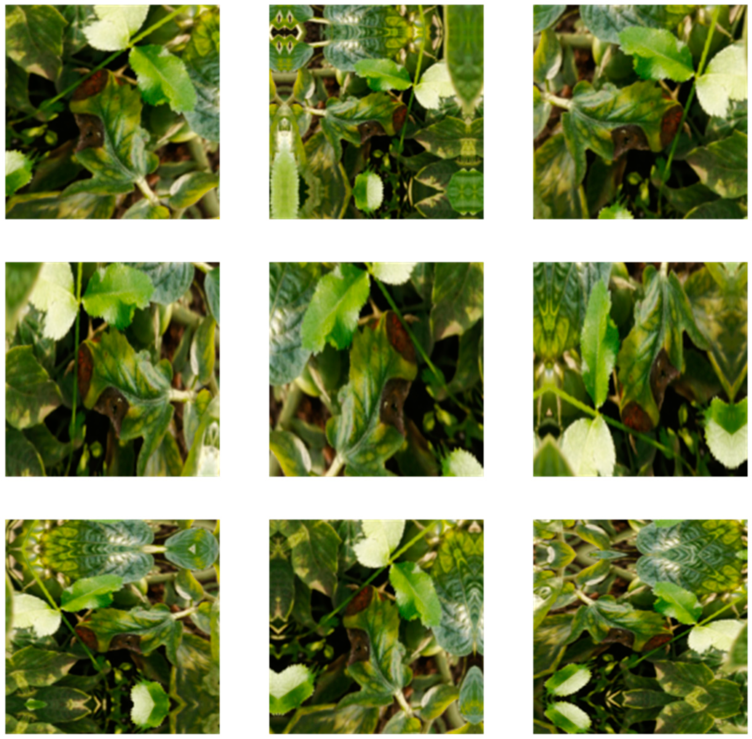
Several methods of data augmentation (flip, rotation, and zoom) were used to create an anomaly dataset to be used in training the models under study until the model learned to detect anomalies. The commands of RandomFlip, RandomRotation, and RandomZoom were used to flip the image horizontally by inverting the pixel columns in the image, to rotate the image clockwise with a rotation factor of 0.2, and to create zoomed-in and zoomed-out images set to ratios (0.5, 0.2), respectively, so the image was reduced by 50% and enlarged by 120%. The three commands were applied together to the same image each time resulting in images that were mirrored, rotated, and zoomed in/out. Figure 3 shows images of tomato disease leaves taken in the field after applying data augmentation to them in 9 different positions. Moreover, it has been noticed that background noise for images that have been zoomed out or rotated resulted in unnecessary features, which were overcome with dropouts.

2.3. Convolutional Neural Network (CNN)

When building a new model, CNN consists of several layers. A CNN contains convolutional, batch normalization, activation, and pooling layers, which are used to discover image features. It also contains dense and dropout layers, which are used to categorize images based on the generated features. CNN is then trained by determining the optimal weights of the neural network to reduce the tolerances between the expected output and the actual input of the dataset used. Loss and optimization functions play an important role in the backpropagation process, which is a typical approach to training neural networks [20]. It has been demonstrated that CNN outperforms traditional feature extraction methods in the identification of plant diseases [2,34]. A typical CNN architecture is described as follows:
Convolutional layers: They contain a collection of common filters or kernels that are used to extract features from pictures by moving the kernel over the image and looking for features to create feature maps. During network training using the backpropagation technique, filters are established from the examples and are thought of as weights. These layers aim to reduce the number of parameters while maintaining network efficiency.
Batch normalization layers: they speed up the training of deep neural networks, as they break down data into mini-batches during normalization to reduce system training complexity. Each feature z is re-measured according to the equation:
z n o r m ( i ) = z ( i ) μ B σ B 2 ε
where ε is a very small positive number that prevents division by zero, and μ B   is the average of the mini-batch mean and σ B 2   represents the mini-batch variance, since the value of z in the first layer is calculated according to the equation:
z = ω x + b
where x is the value of the input features, b is the bias.
To scale and shift the normalized inputs γ , and   β are added and learned using the network parameters through the equation:
z ˜ ( i ) = γ z n o r m ( i ) + β
Activation layers: The activation function is used to speed up arithmetic operations without going through the problems of vanishing or exploiting. The rectified linear unit (ReLU) was used as the basic activation function, which is one of the most widely used activation functions. It is characterized by the ease and simplicity of its equation and it transforms the previous z ˜ using the mathematical model:
a =   max ( 0 ; z ˜ )
The use of the final activation function differs in that it is used as the output of the last dense layer. It shows the prediction probabilities as either 0 or 1 in the case of binary classification, or as a decimal percentage in the case of multiple classification. The SoftMax function was used to assign decimal probabilities to each class. It is calculated from the output unit i according to the equation:
a ( i ) = e z ( i ) i m e z ( i )   for   i = 1 ,   2 ,   3 , , m
where z ( i ) is the output of the i dimension, a ( i ) is the probability related to the i class, and m is the number of dimensions corresponding to the number of classes. A sample is assigned to the class with the highest probability when predicting by the method described below:
y i ^ = max i [ 1 , m ] a ( i )
Pooling layers: Reduces the dimensions of feature maps, as it selects the most important features from the features created by the convolution layers. There are two types of pooling layers: average pooling and maximum pooling. Average pooling takes the average value of each feature map, while maximum pooling takes the largest value.
Fully connected layers: This consists of neurons and forms the last layers of the neural network, where it takes its inputs from the final output of the pooling or convolutional layers and turns it into a single vector by means of a flatten layer. Then, it makes a prediction using weights and the final probabilities are given by a dense layer. The number of cells in the last dense layer corresponds to the number of classes.
Dropout layers: they are a regularization technique mostly used during network training to avoid overfitting by deleting a portion of the incoming neurons and their connections.
A loss function: another name for the cost function. It is computed by cross-entropy (CE) to find the loss between the actual output y and the expected output y ^ . CE in multiple classifications is calculated according to the equation:
L cross _ entropy   ( y ^ , y ) = j = 0 K y j log ( y j ^ )               f o r   j = 1 ,   2 ,   3 k  
where K is the number of classes.
An Optimization function: This is used to reduce the loss function using one of the optimization functions since the Adam optimizer was used in this work. The Adam optimizer learns weights adaptively.

2.4. Inception V3 and Inception ResNet V2 Models

In this paper, the Inception V3 and the Inception ResNet V2 models were used for pre-training. The Inception V3 model is an additional development design for a usable CNN created by Google. Inception begins with estimating a sparse structure, increasing network depth and width, and clustering sparse data into a dense structure to enhance accuracy without putting too much burden on computer resources [35]. Whereas the Inception ResNet V2 model combines GoogLeNet (Inception) and ResNet. ResNet’s fundamental concept is to create a direct link to the framework known as the highway network concept. The highway network allows a certain percentage of the output from the previous network layer to be retained, even though the previous network structure is a non-linear modification of the performance input. It enables the next layer to receive the original input data immediately. Meanwhile, ResNet can ensure information integrity by transferring data directly from input to output [36].
Transitional learning is a machine learning technique that involves re-modeling a task related to the task being trained. Transfer learning as shown in Figure 4 was used to transfer plant pathology data to Inception V3 and Inception ResNet V2 models pre-trained on imagenet data to speed up the training process and improve model performance. The Inception V3 network contains 94 convolutional layers, 14 pooling layers, and a dense layer [37]. Whereas, Inception ResNet V2 contains 132 convolutional layers, 5 pooling layers, and a dense layer [38]. Transfer learning from a pre-trained CNN model includes two techniques, feature extraction and fine-tuning which are often used together in a variety of applications to achieve the best results. In this paper, feature extraction and fine-tuning were used together, where feature extraction was first used to train the new classifier. Then, fine-tuning was used to retrain half of the layers of the network’s convolutional phase. Inception V3 and Inception ResNet V2 models were trained using the training parameters shown in Table 3.
In this paper, an average pooling layer and a dense layer were added. Then, SoftMax was added as an activation function for the last layer set, with the number of classes determined. After that, the dropout rate was used to train the models. The next step is determining the learning rate and Adam as the optimizer, and the epochs were specified as 15 for the train and 25 for the fine-tuning. The Inception V3 model consists of 6147 trainable parameters during CNN training and 16,344,963 trainable parameters during fine-tuning. While the Inception ResNet V2 model contains 4611 trainable parameters during CNN training and 41,357,763 trainable parameters during fine-tuning. The Inception V3 and Inception ResNet V2 models used to diagnose tomato diseases are summarized in Table 4.
The CNNs’ numerous parameters make it possible for overfitting issues to develop in these networks through the dropout procedure. Dropout is a random disconnecting technique that has a 1-p dropout probability and can randomly isolate the connections between various nodes. The dropout layer decreases the number of model parameters and boosts the algorithm’s robustness. The random inactivation layer enhances the robustness of the network structure and enables the model to prevent overfitting from occurring [39]. Recently, dropout has been used to lessen deep neural network overfitting. Dropout randomly disables a certain number of neurons in each layer at random during each epoch, using only the remaining neurons for both forward and backward propagations. As a result, the active neurons become more resilient and are motivated to extract useful features independently and more successfully without the assistance of the inactive ones. As a result, the joint adaptability of neurons is reduced while the ability of the entire network to generalize is increased [40]. In this work, different dropout rates at 5%, 10%, 15%, 20%, 25%, 30%, 40%, and 50% were studied. Since the data used is relatively large, dropout rates up to 50% have been studied.

2.5. Evaluation

Two assessment indicators commonly used in classification issues were used to assess the predictive strength of the proposed approach: confusion matrix, and accuracy for comparing models when training, validation, and testing.
The confusion matrix is a table that shows how well a classification model performs on a test set by matching the expected outputs with the actual outputs to identify the correct values.
Accuracy is the percentage of valid predictions resulting from all forecasts made, usually expressed as a percentage and determined using an equation:
Accuracy = Number   of   correct   prediction Total   number   of   prediction   = TP +   TN TP +   TN +   FP +   FN
where TP, TN, FP, and FN are true positive, true negative, false positive, and false negative, respectively.

3. Results

The CNN models mentioned in Section 2.4 were trained using the parameters presented in Table 3. The dropout ratios listed in Table 3 were used to train each model. The models were compared using accuracy, loss to train, and validation and testing, and the results were summarized in Table 5. It is clear from the table that there are no noticeable differences between the two models during the different dropout rates because the differences are slight, the accuracy values are close to 97.8–99.2% and there are slight differences in the loss values for the different dropouts. Moreover, the models used are good for detecting tomato diseases at different dropout rates. We note that at a 5% dropout rate, the loss value in the Inception V3 model and the Inception ResNet V2 model is 0.0685 and 0.0438, respectively. Moreover, Inception ResNet V2 is better than Inception V3 at a 5%, 10%, and 15% dropout rate, but Inception V3 is better than Inception ResNet V2 at the rest of the dropout rates. Additionally, at a 20% dropout rate, there are no noticeable differences in the loss values in both models. It was also observed that the lowest percentage of loss in the Inception V3 model with a value of 0.0234 at a dropout rate of 30%, while the lowest percentage of loss in the Inception ResNet V2 model at a dropout rate of 15% with a value of 0.0309. Moreover, the highest accuracy rate is 99.22% in the Inception V3 model at a dropout rate of 50%. This percentage was also achieved in the Inception ResNet V2 model at a dropout rate of 15% and 25%. So, the Inception V3 model with a 50% dropout rate and the Inception ResNet V2 model with a 15% dropout rate are the best models. They achieve less loss than the Inception ResNet V2 model at a 25% dropout.
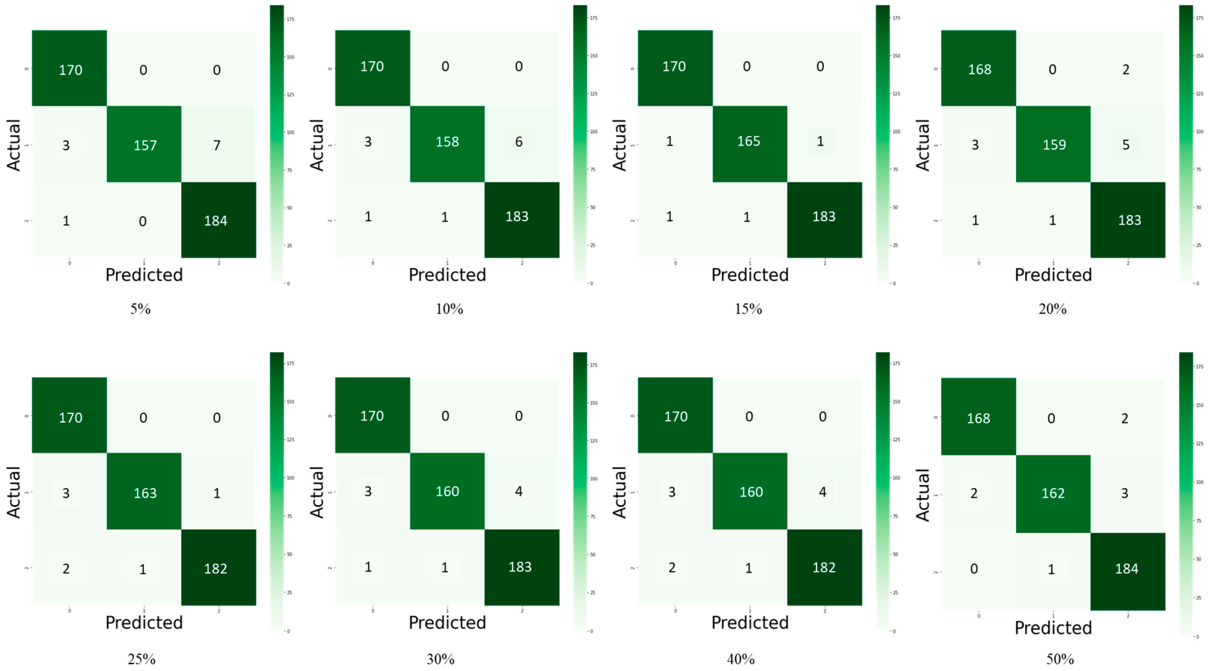
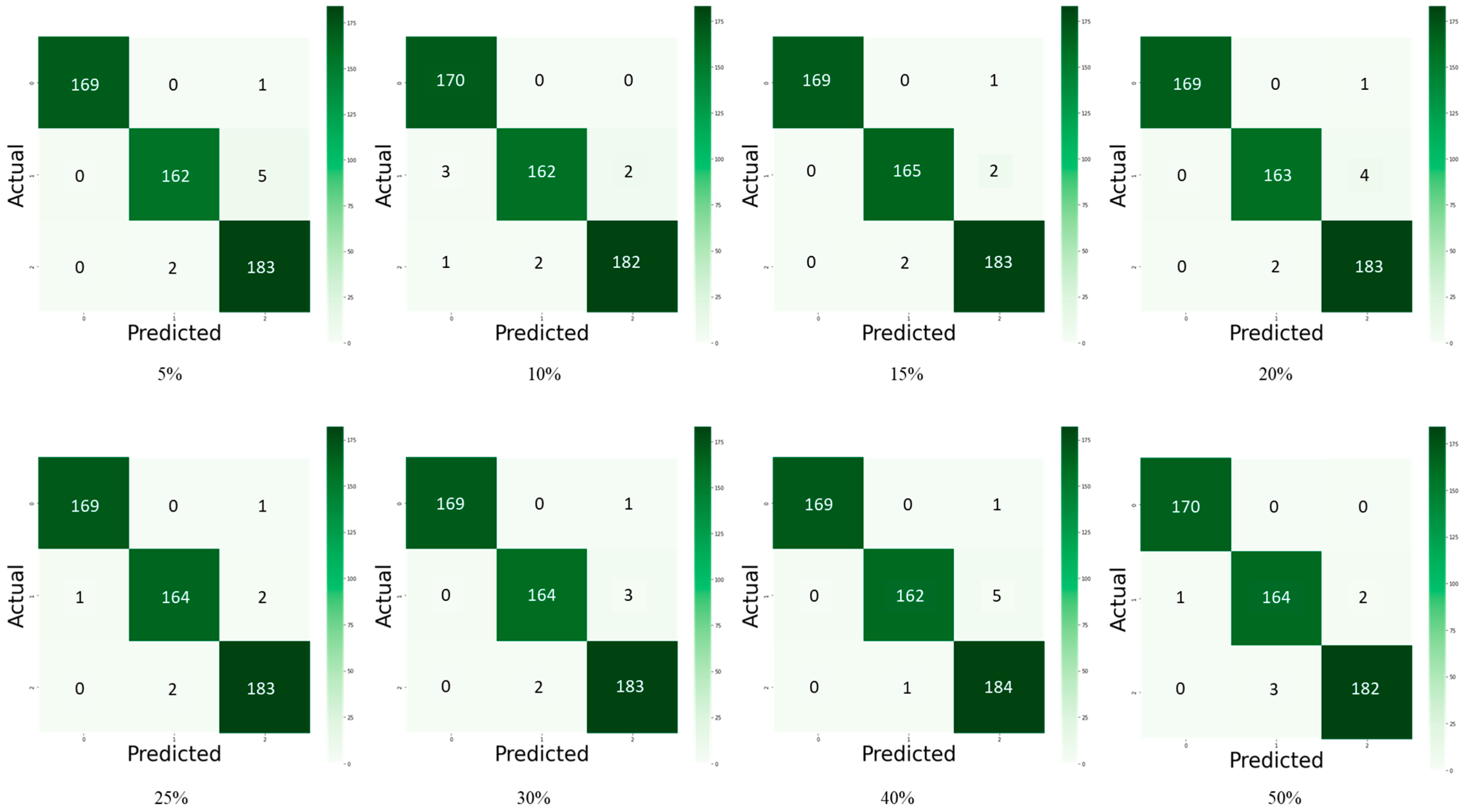
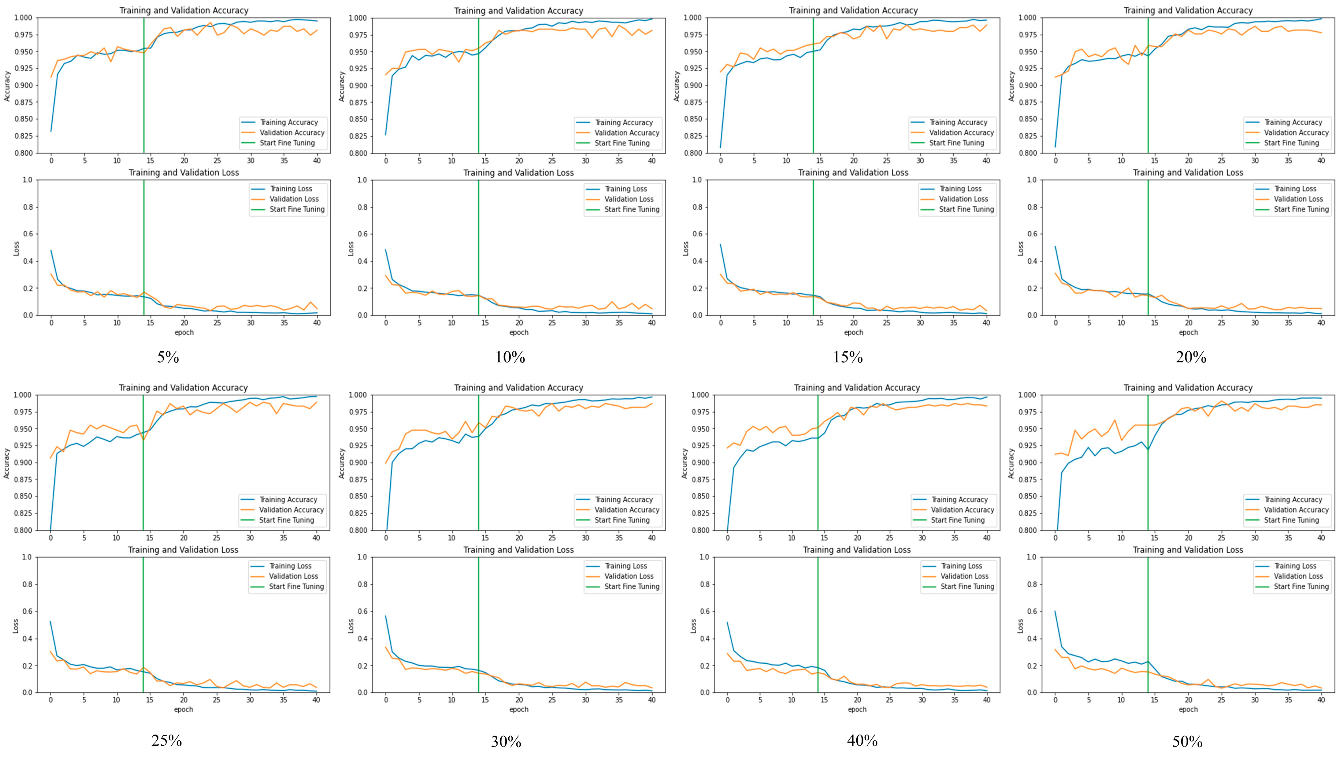
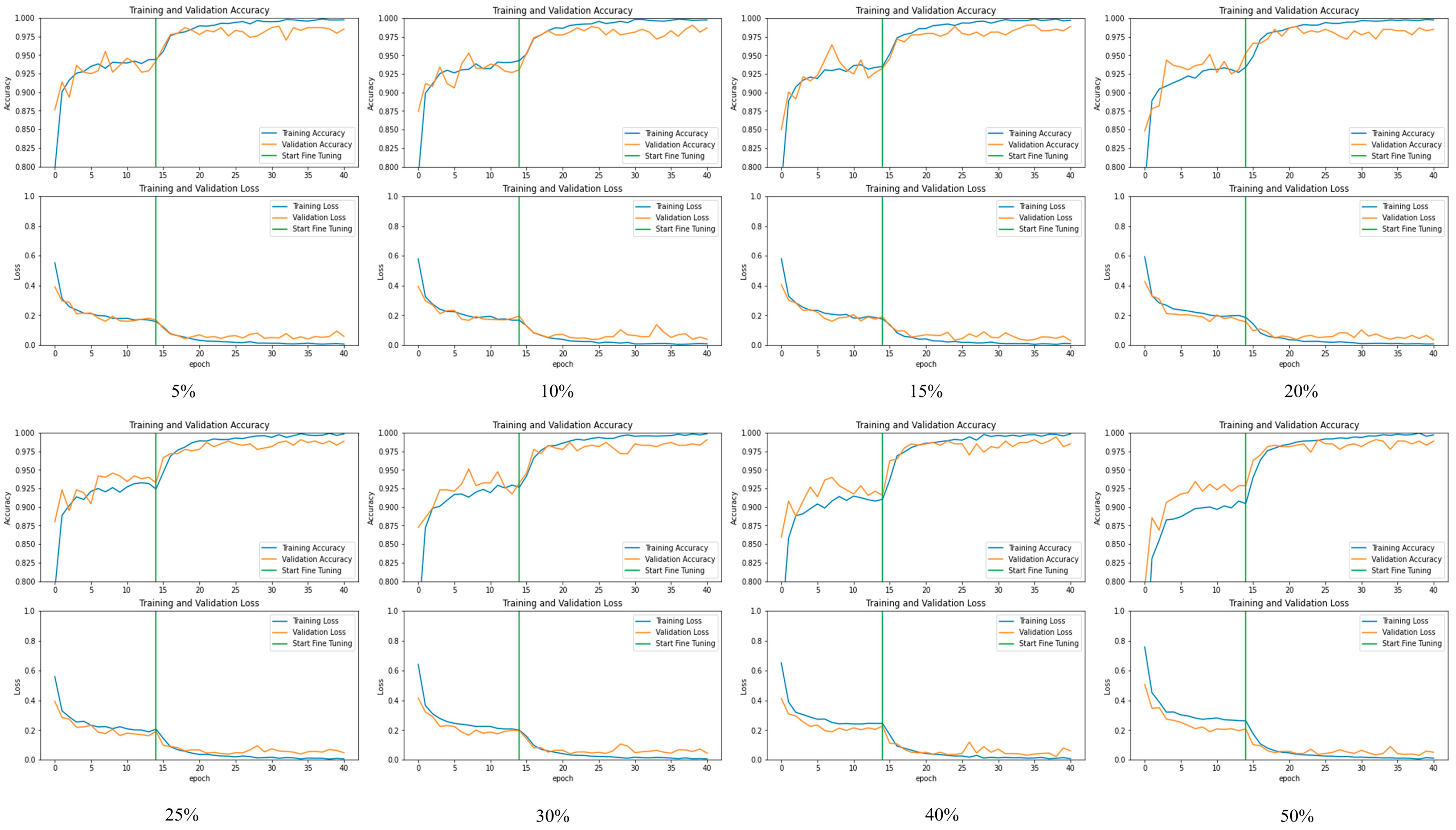
Figure 5 and Figure 6 depict the confusion matrix for the models used by the different dropouts, and it is clear that there are no high differences between the models used. Figure 7 and Figure 8 show the change in both accuracy and loss of the models used at different dropouts, and we also note that the train operation is significantly improved after fine-tuning. At the same time, fine-tuning speeds up training. In addition to the above, the results indicate that the models used at different dropouts have a great ability to identify tomato diseases. In particular, the models not only used healthy and diseased plants but also identified certain classes of plant diseases. Thus, based on the empirical analysis, it can be concluded that the models used at different dropouts are effective in identifying tomato diseases. It can also be extended to detect other plant diseases. Moreover, it can be extended to the application of other fields such as online fault diagnosis, target recognition, etc.

4. Performance Analysis

The Inception V3 and Inception ResNet V2 models’ performance are compared to existing methods reported in the literature, and the resulting observations, sorted by accuracy obtained, are highlighted in Table 6. Recent deep learning studies used well-trained architectures such as DenseNet, ResNet, GoogleNet, and others to detect disease in tomato leaves [21,22,23,24,25,30]. These works achieve remarkable results, and the accuracy of these works ranges from 91% to 99% and because the proposed models used transfer learning technology, they were also able to achieve a high accuracy of up to 99%, which is a significant improvement over other works. In addition, images from the field and PlantVillage were used to train the models in this study, in contrast to the other existing works in which only PlantVillage images were used.

5. Conclusions

In this work, two deep neural networks were used to diagnose tomato leaf diseases on a set of laboratory and field data. Image pre-processing and data augmentation were performed. Then, the Inception V3 and the Inception ResNet V2 models were retrained using transfer learning. By removing the last layers of the models and replacing them with average pooling, fully connected, and softmax layers, respectively. Whereas different dropout rates for the previous models were used at rates of 5%, 10%, 15%, 20%, 25%, 30%, 40%, and 50%. The results of the experiments showed that the models used are very competitive and show a high degree of accuracy close to 99.22%. When using the dropout rates for both models, the Inception V3 model with a 50% dropout rate and the Inception ResNet V2 model with a 15% dropout rate gave the best performance with an accuracy of 99.22% and a loss of 0.03.

Author Contributions

Conceptualization, A.S.; Software, A.S.; Writing—original draft, A.S.; Writing—review & editing, A.M., M.A.A. and A.Y.A.; Visualization, M.M.; Supervision, A.A.A.-A., A.M. and M.M.; Project administration, A.M. and M.M. All authors have read and agreed to the published version of the manuscript.

Funding

This research received no external funding.

Institutional Review Board Statement

Not applicable.

Data Availability Statement

Not applicable.

Conflicts of Interest

The authors declare no conflict of interest.

References

  1. Wspanialy, P.; Moussa, M. A detection and severity estimation system for generic diseases of tomato greenhouse plants. Comput. Electron. Agric. 2020, 178, 105701. [Google Scholar] [CrossRef]
  2. Mohanty, S.P.; Hughes, D.P.; Salathé, M. Using Deep Learning for Image-Based Plant Disease Detection. Front. Plant Sci. 2016, 7, 1419. [Google Scholar] [CrossRef] [PubMed] [Green Version]
  3. Ferentinos, K.P. Deep learning models for plant disease detection and diagnosis. Comput. Electron. Agric. 2018, 145, 311–318. [Google Scholar] [CrossRef]
  4. Lins, E.A.; Rodriguez, J.P.; Scoloski, S.I.; Pivato, J.; Lima, M.B.; Fernandes, J.M.; da Silva Pereira, P.R.; Lau, D.; Rieder, R. A method for counting and classifying aphids using computer vision. Comput. Electron. Agric. 2020, 169, 105200. [Google Scholar] [CrossRef]
  5. Griffel, L.M.; Delparte, D.; Edwards, J. Using Support Vector Machines classification to differentiate spectral signatures of potato plants infected with Potato Virus Y. Comput. Electron. Agric. 2018, 153, 318–324. [Google Scholar] [CrossRef]
  6. LeCun, Y.; Bengio, Y.; Hinton, G. Deep learning. Nature 2015, 521, 436–444. [Google Scholar] [CrossRef] [PubMed]
  7. da Silva, G.L.F.; da Silva Neto, O.P.; Silva, A.C.; de Paiva, A.C.; Gattass, M. Lung nodules diagnosis based on evolutionary convolutional neural network. Multimed. Tools Appl. 2017, 76, 19039–19055. [Google Scholar] [CrossRef]
  8. Lecun, Y. Gradient-Based Learning Applied to Document Recognition. Proc. IEEE 1998, 86, 2278–2324. [Google Scholar] [CrossRef] [Green Version]
  9. Cui, C.; Fearn, T. Modern practical convolutional neural networks for multivariate regression: Applications to NIR calibration. Chemom. Intell. Lab. Syst. 2018, 182, 9–20. [Google Scholar] [CrossRef]
  10. Rawat, W.; Wang, Z. Deep Convolutional Neural Networks for Image Classification: A Comprehensive Review. Neural Comput. 2017, 29, 2352–2449. [Google Scholar] [CrossRef]
  11. Abdulnabi, A.H.; Wang, G.; Lu, J.; Jia, K. Multi-Task CNN Model for Attribute Prediction. IEEE Trans. Multimed. 2015, 17, 1949–1959. [Google Scholar] [CrossRef] [Green Version]
  12. Russakovsky, O.; Deng, J.; Su, H.; Krause, J.; Satheesh, S.; Ma, S.; Fei-Fei, L. ImageNet Large Scale Visual Recognition Challenge. Int. J. Comput. Vis. 2015, 115, 211–252. [Google Scholar] [CrossRef] [Green Version]
  13. Kong, J.; Wang, H.; Wang, X.; Jin, X.; Fang, X.; Lin, S. Multi-stream hybrid architecture based on cross-level fusion strategy for fine-grained crop species recognition in precision agriculture. Comput. Electron. Agric. 2021, 185, 106134. [Google Scholar] [CrossRef]
  14. Wu, F.; Duan, J.; Chen, S.; Ye, Y.; Ai, P.; Yang, Z. Multi-Target Recognition of Bananas and Automatic Positioning for the Inflorescence Axis Cutting Point. Front. Plant Sci. 2021, 12, 705021. [Google Scholar] [CrossRef]
  15. Ahmed, I.; Yadav, P.K. Plant disease detection using machine learning approaches. Expert Syst. 2022. [Google Scholar] [CrossRef]
  16. Andayani, P.Y.; Franz, A.; Nurlaila, N. Expert System for Diagnosing Diseases Cocoa Using the Dempster Shafer Method. Tepian 2020, 1, 35–43. [Google Scholar]
  17. Tan, H.Y.; Goh, Z.Y.; Loh, K.-H.; Then, A.Y.-H.; Omar, H.; Chang, S.-W. Cephalopod species identification using integrated analysis of machine learning and deep learning approaches. PeerJ 2021, 9, 11825. [Google Scholar] [CrossRef]
  18. Zhang, M.; Dong, L. Review of Application Research of Expert System and Neural Network in Credit Risk Evaluation. In Proceedings of the 3rd Annual 2017 International Conference on Management Science and Engineering (MSE 2017), Guilin, China, 18–20 August 2017. [Google Scholar] [CrossRef] [Green Version]
  19. Zhuang, S.; Wang, P.; Jiang, B.; Li, M. Learned features of leaf phenotype to monitor maize water status in the fields. Comput. Electron. Agric. 2020, 172, 105347. [Google Scholar] [CrossRef]
  20. Darwish, A.; Ezzat, D.; Hassanien, A.E. An optimized model based on convolutional neural networks and orthogonal learning particle swarm optimization algorithm for plant diseases diagnosis. Swarm Evol. Comput. 2020, 52, 100616. [Google Scholar] [CrossRef]
  21. Abbas, A.; Jain, S.; Gour, M.; Vankudothu, S. Tomato plant disease detection using transfer learning with C-GAN synthetic images. Comput. Electron. Agric. 2021, 187, 106279. [Google Scholar] [CrossRef]
  22. Zhang, K.; Wu, Q.; Liu, A.; Meng, X. Can Deep Learning Identify Tomato Leaf Disease? Adv. Multimed. 2018, 2018, 6710865. [Google Scholar] [CrossRef] [Green Version]
  23. Widiyanto, S.; Fitrianto, R.; Wardani, D.T. Implementation of Convolutional Neural Network Method for Classification of Diseases in Tomato Leaves. In Proceedings of the 2019 Fourth International Conference on Informatics and Computing (ICIC), Semarang, Indonesia, 16–17 October 2019; pp. 1–5. [Google Scholar] [CrossRef]
  24. Barbedo, J.G.A. Plant disease identification from individual lesions and spots using deep learning. Biosyst. Eng. 2019, 180, 96–107. [Google Scholar] [CrossRef]
  25. Agarwal, M.; Singh, A.; Arjaria, S.; Sinha, A.; Gupta, S. ToLeD: Tomato Leaf Disease Detection using Convolution Neural Network. Procedia Comput. Sci. 2020, 167, 293–301. [Google Scholar] [CrossRef]
  26. Tm, P.; Pranathi, A.; SaiAshritha, K.; Chittaragi, N.B.; Koolagudi, S.G. Tomato Leaf Disease Detection Using Convolutional Neural Networks. In Proceedings of the 2018 Eleventh International Conference on Contemporary Computing (IC3), Noida, India, 2–4 August 2018; pp. 1–5. [Google Scholar] [CrossRef]
  27. Chen, H.; Chen, A.; Xu, L.; Xie, H.; Qiao, H.; Lin, Q.; Cai, K. A deep learning CNN architecture applied in smart near-infrared analysis of water pollution for agricultural irrigation resources. Agric. Water Manag. 2020, 240, 106303. [Google Scholar] [CrossRef]
  28. Fan, X.; Luo, P.; Mu, Y.; Zhou, R.; Tjahjadi, T.; Ren, Y. Leaf image based plant disease identification using transfer learning and feature fusion. Comput. Electron. Agric. 2022, 196, 106892. [Google Scholar] [CrossRef]
  29. Yu, H.; Liu, J.; Chen, C.; Heidari, A.A.; Zhang, Q.; Chen, H. Optimized deep residual network system for diagnosing tomato pests. Comput. Electron. Agric. 2022, 195, 106805. [Google Scholar] [CrossRef]
  30. Karthik, R.; Hariharan, M.; Anand, S.; Mathikshara, P.; Johnson, A.; Menaka, R. Attention embedded residual CNN for disease detection in tomato leaves. Appl. Soft Comput. 2020, 86, 105933. [Google Scholar] [CrossRef]
  31. Hughes, D.P.; Salathé, M. An open access repository of images on plant health to enable the development of mobile disease diagnostics. arxiv 2015, arXiv:1511.08060. [Google Scholar]
  32. AbdElfatah, H.-A.S.; Sallam, N.M.A.; Mohamed, M.S.; Bagy, H.M.M.K. Curvularia lunata as new causal pathogen of tomato early blight disease in Egypt. Mol. Biol. Rep. 2021, 48, 3001–3006. [Google Scholar] [CrossRef]
  33. Kil, E.J.; Byun, H.S.; Hwang, H.; Lee, K.Y.; Choi, H.S.; Kim, C.S.; Lee, S. Tomato Yellow Leaf Curl Virus Infection in a Monocotyledonous Weed (Eleusine indica). Plant Pathol. J. 2021, 37, 641–651. [Google Scholar] [CrossRef]
  34. Chen, J.; Chen, J.; Zhang, D.; Sun, Y.; Nanehkaran, Y.A. Using deep transfer learning for image-based plant disease identification. Comput. Electron. Agric. 2020, 173, 105393. [Google Scholar] [CrossRef]
  35. Al Husaini, M.A.S.; Habaebi, M.H.; Gunawan, T.S.; Islam, M.R.; Elsheikh, E.A.A.; Suliman, F.M. Thermal-based early breast cancer detection using inception V3, inception V4 and modified inception MV4. Neural Comput. Appl. 2022, 34, 333–348. [Google Scholar] [CrossRef] [PubMed]
  36. Chen, J.; Yang, T.; Zhang, D.; Huang, H.; Tian, Y. Deep learning based classification of rock structure of tunnel face. Geosci. Front. 2021, 12, 395–404. [Google Scholar] [CrossRef]
  37. Szegedy, C.; Vanhoucke, V.; Ioffe, S.; Shlens, J.; Wojna, Z. Rethinking the Inception Architecture for Computer Vision. arXiv 2015, arXiv:1512.00567. [Google Scholar]
  38. Szegedy, C.; Ioffe, S.; Vanhoucke, V.; Alemi, A. Inception-v4, Inception-ResNet and the Impact of Residual Connections on Learning. arXiv 2016, arXiv:1602.07261. [Google Scholar] [CrossRef]
  39. Munir, N.; Kim, H.-J.; Song, S.-J.; Kang, S.-S. Investigation of deep neural network with drop out for ultrasonic flaw classification in weldments. J. Mech. Sci. Technol. 2018, 32, 3073–3080. [Google Scholar] [CrossRef]
  40. Srivastava, N.; Hinton, G.; Krizhevsky, A.; Sutskever, I.; Salakhutdinov, R. Dropout: A Simple Way to Prevent Neural Networks from Overfitting. J. Mach. Learn. Res. 2014, 15, 1929–1958. [Google Scholar]
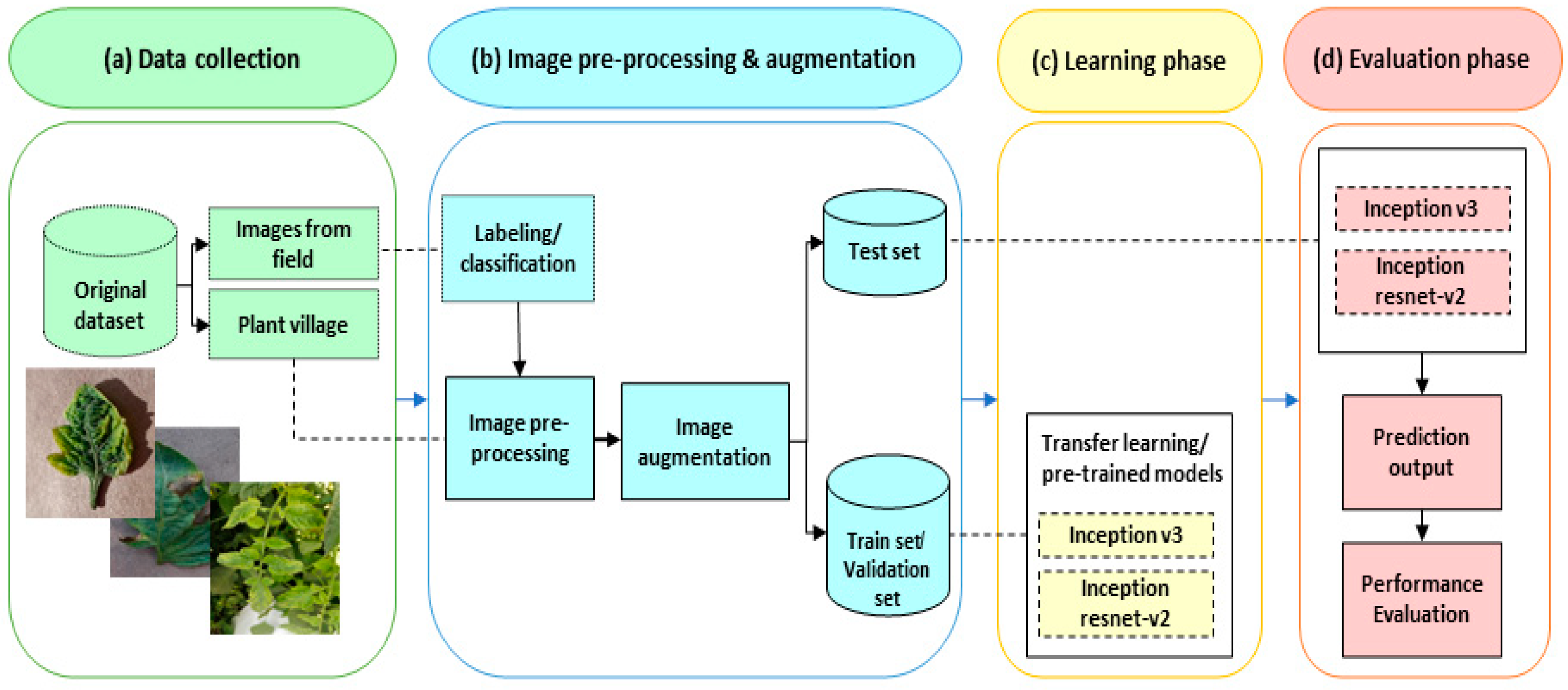
Figure 1. Diagram for identifying tomato leaf diseases.
Agriculture 13 00139 g001
Figure 2. Sample images of the tomato Leaf dataset: (A) Early Blight; (B) Yellow Leaf Curl Virus; and (C) Health.
Agriculture 13 00139 g002
Figure 3. Data augmentation for field-captured images of tomato leaf diseases. The image appears in different positions using flipping, rotation, and zooming together with randomly chosen values.
Agriculture 13 00139 g003
Figure 4. CNN architecture to develop a pre-trained model for tomato disease diagnosis.
Agriculture 13 00139 g004
Figure 5. Confusion matrix of tomato leaf disease detection for Inception V3 model with 5%, 10%, 15%, 20%, 25%, 30%, 40%, and 50% dropout values, numbers represent the classes used for testing where: 0 = Early Blight, 1 = Yellow Leaf Curl Virus, and 2 = Healthy.
Agriculture 13 00139 g005
Figure 6. Confusion matrix of tomato leaf disease detection for Inception ResNet V2 model with 5%, 10%, 15%, 20%, 25%, 30%, 40%, and 50% dropout values, numbers represent the classes used for testing where: 0 = Early Blight, 1 = Yellow Leaf Curl Virus, and 2 = Healthy.
Agriculture 13 00139 g006
Figure 7. The relationship between accuracy and loss with the number of epochs for the dataset before and after fine-tuning the Inception V3 model with 5%, 10%, 15%, 20%, 25%, 30%, 40%, and 50% dropout values.
Agriculture 13 00139 g007
Figure 8. The relationship between accuracy and loss with the number of epochs for the dataset before and after fine-tuning Inception ResNet V2 model at 5%, 10%, 15%, 20%, 25%, 30%, 40%, and 50% dropout values.
Agriculture 13 00139 g008
Table 1. Number of images used in the study for each category.
CategoryDisease NameImages from PlantVillage
(Number)
Images Captured from the Field (Number)
0Early Blight1000814
1Yellow Leaf Curl Virus938544
2Healthy1591338
Total35291696
Table 2. Description of the tomato diseases included in the study, defining each disease, and describing its symptoms.
ClassDescription
Early Blight
  • Destructive fungal disease of tomato and potato plants.
  • Initially appear on the lower leaves as plants age.
  • They resemble small, dark necrotic lesions with concentric rings that resemble targets and are frequently encircled by a yellowing zone [32].
Yellow Leaf Curl Virus
  • Infecting virus known as Tomato Yellow Leaf Curl Virus (TYLCV, Genus Begomovirus, Family Geminiviridae).
  • Spread by whiteflies (Bemisia tabaci).
  • Losses can occur when tomato plants with TYLCV infection display serious symptoms such as interveinal yellowing, curled leaves, and significantly stunted development [33].
Table 3. Parameters value used to build tomato disease diagnosis models for the CNN training and fine-tuning phases.
ParameterValue
Batch Size32
Dropout5%, 10%, 15%, 20%, 25%, 30%, 40%, and 50%
Activation functionReLU, SoftMax
OptimizerAdam
CNN Training
Epoch15
Learning Rate0.001
Fine-tuning
Epoch25
Learning Rate0.00001
Table 4. Summary of tomato disease diagnoses models.
Type of LayerInception V3Inception ResNet V2
Output ShapeParametersOutput ShapeParameters
CNN Training
Input(299, 299, 3)0(299, 299, 3)0
Sequential(299, 299, 3)0(299, 299, 3)0
Functional
(Inception V3, Inception ResNet V2)
(8, 8, 2048)21,802,784(8, 8, 1536)54,336,736
Average Pooling(0, 2048)0(0, 1536)0
Dropout(0, 2048)0(0, 1536)0
Dense(0, 3)6147(0, 3)4611
Total parameters21,808,93154,341,347
Trainable parameters61474611
Non-trainable parameters21,802,78454,336,736
Fine-Tuning
Trainable parameters16,344,96341,357,763
Non-trainable parameters5,463,96812,983,584
Table 5. Accuracy and loss for the training, validation, and testing phases of Inception V3 and Inception ResNet V2 models with different dropout values.
Drop Out
(%)
TrainValidationTest
Accuracy (%)LossAccuracy (%)LossAccuracy (%)Loss
Inception V3 model
599.330.016697.560.062497.850.0685
1099.570.010398.120.046698.830.0460
1599.950.003499.060.031198.830.0342
2099.550.010797.750.044699.020.0366
2599.900.004698.870.032198.630.0411
3099.810.005998.690.036198.630.0234
4099.830.006198.12 0.033298.630.0308
5099.780.006398.690.025299.220.0318
Inception ResNet V2 model
599.830.004698.310.059899.020.0438
1099.880.003798.870.031498.830.0322
1599.930.002298.870.027799.220.0309
2099.930.002198.690.039298.830.0396
2599.780.006598.690.045799.220.0522
3099.950.002499.060.039899.020.0495
4099.400.012898.500.063298.830.0636
5099.830.005898.500.037999.020.0467
Table 6. Compares the performance of the proposed work to that of other existing works.
No.Author (s)MethodImage NumberImage
Source
Accuracy (%)
1Agarwal et al. (2020) [25]CNN network17,500PlantVillage91.20
2Prajwala Tm et al. (2018) [26]LeNet based CNN18,160PlantVillage95
3Widiyanto et al. (2019) [23]CNN model 5000 PlantVillage96.60
4Keke Zhang et al. (2018) [22]ResNet 5550 PlantVillage97.28
5Karthik et al. (2020) [30]Attention-based Residual CNN95,999PlantVillage98
6Abbas et al. (2021) [21]DenseNet, C-GAN16,012PlantVillage99.51
7Proposed approachInception V3 and Inception ResNet V2 5225 PlantVillage and field99.22
Disclaimer/Publisher’s Note: The statements, opinions and data contained in all publications are solely those of the individual author(s) and contributor(s) and not of MDPI and/or the editor(s). MDPI and/or the editor(s) disclaim responsibility for any injury to people or property resulting from any ideas, methods, instructions or products referred to in the content.