A Time Series-Based Point Estimation of Stop Signal Reaction Times: More Evidence on the Role of Reactive Inhibition-Proactive Inhibition Interplay on the SSRT Estimations †

 ,
,  , , and
Abstract
1. Introduction
2. Methods and Materials
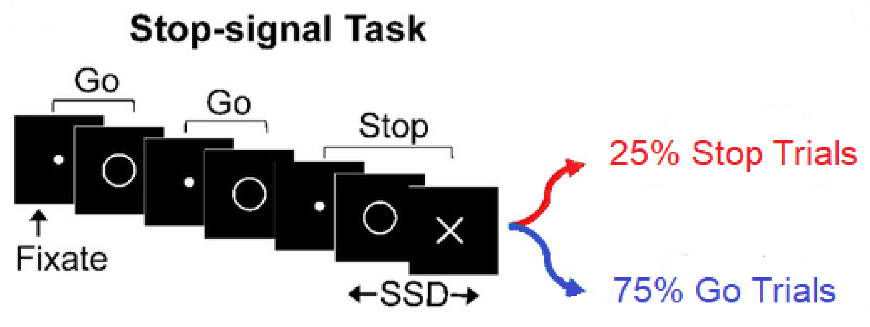
2.1. Data
2.1.1. The Real Data
2.1.2. The Simulated Data
2.2. Participants
2.3. Statistical Inference
2.3.1. Time Series Based State- Space SSRT (SSRTSS.Logan1994)
2.3.2. Inhibition Indices and Hypothesis Tests
3. Results
3.1. Disparities of the Internal Inhibition Indices
3.2. Time Series Based State-Space SSRT for the Real SST Data
3.3. Simulations and Asymptotic Behaviour
- Result (i):
- The difference between the and in the simulated data is the same as in the original real data. However, the size of differences in the former (8.1–11.8 ms) is smaller than the latter (13.1 ms), and with increasing simulated sample sizes, their gap diminishes.
- Result (ii):
- The difference between and in the simulated data is in the range 8.5–11.7 ms and very different from the non-significant difference in the original real data.
- Result (iii):
- The difference between and in the simulated data is in the range of 4.0–5.4 ms, and somewhat different than that of their non-significant difference in real data.
- Result (i):
- The difference between and in the simulated data (8.1 ms–11.8 ms) is significantly smaller than in the original real data (21.9).
- Result (ii):
- The difference between the and in the simulated data (8.1 ms–11.8 ms) is similar to that of the real data (8.3 ms).
- Result (iii):
- The difference between and in the simulated data (8.1 ms–11.8 ms) is similar to that of real data (7.7 ms).
4. Discussion
5. Conclusions
Author Contributions
Funding
Acknowledgments
Conflicts of Interest
Abbreviations
| ADHD | Attention Deficit Hyperactivity Disorder |
| AXCPT | AX Continuous Performance Task |
| CSST | Conditional Stop Signal Task |
| EM | Expectation Maximization |
| GORT | Reaction time in a go trial |
| GORTA | Reaction time in a type A go trial |
| GORTB | Reaction time in a type B go trial |
| LMM | Linear Mixed Model |
| RT | Reaction Times |
| SI | Successful Inhibition |
| SR | Signal Respond |
| SRRT | Reaction time in a failed stop trial |
| SSAT | Stop Signal Anticipation Task |
| SSD | Stop Signal Delay |
| SSRT | Stop Signal Reaction Times in a stop trial |
| SSRTA | Stop Signal Reaction Times in type A stop trial |
| SSRTB | Stop Signal Reaction Times in type B stop trial |
| SSRTLogan1994 | Logan 1994 SSRT |
| SSRTMixture | Mixture SSRT |
| SSRTSS.Logan1994 | Time Series-based State-Space SSRT |
| SSRTWeighted | Weighted SSRT |
| SSST | Standard Stop Signal Task |
| SST | Stop Signal Task |
| SWAN | Strengths and Weakness of ADHD-symptoms and Normal behavior rating scale |
Appendix A. R Software Simulation Code of Stop Signal Task Data with Tracking Method
Appendix B. Cluster Type Weight Calculations in the Simulation of SST Data
References
- Logan, G.D. On the Ability to Inhibit Thought and Action: A User’s Guide to the Stop Signal Paradigm. In Inhibitory Process in Attention, Memory and Language; Dagenbach, D., Carr, T.H., Eds.; Academic Press: San Diego, CA, USA, 1994. [Google Scholar]
- Verbruggen, F.; Aron, A.R.; Band, G.P.; Beste, C.; Bissett, P.G.; Brockett, A.T.; Brown, J.W.; Chamberlain, S.R.; Chambers, C.D.; Colonius, H.; et al. Capturing the ability to inhibit actions and impulsive behaviours: A Consensus Guide to the Stop Signal Task. Elife 2019, 8. [Google Scholar] [CrossRef] [PubMed]
- Bartholly, S.; Rennalls, S.J.; Jacques, C.; Danby, H.; Campbell, I.C.; Schmidt, U.; O’Daly, O.G. Proactive and reactive inhibitory control in eating disorders. Psychiatry Res. 2017, 255, 432–440. [Google Scholar] [CrossRef] [PubMed]
- Van Voorhis, A.C.; Kent, J.S.; Kang, S.S.; Goghani, V.M.; MacDonald, A.W., 3rd; Sponheim, S.R. Abnormal neural functions associated with motor inhibition deficits in schizophrenia and bipolar disorder. Hum. Brain Mapp. 2019, 40, 5397–5411. [Google Scholar] [CrossRef] [PubMed]
- Castro-Meneses, L.J.; Johnson, B.W.; Sowman, D.F. The effects of impulsivity and proactive inhibition on reactive inhibition and the go process: Insights from vocal and manual Stop Signal Tasks. Front. Hum. Neurosci. 2018, 9, 529. [Google Scholar] [CrossRef] [PubMed]
- Brevers, D.; Dubuisson, E.; Dejonghe, F.; Dutrieux, J.; Petieau, M.; Cheron, G.; Verbanck, P.; Foucart, J. Proactive and Reactive Motor Inhibition in Top Athletes Versus Nonathletes. Percept. Mot. Ski. 2018, 125, 289–312. [Google Scholar] [CrossRef]
- Zandbelt, B.B.; Bloemendaal, M.; Neggers, S.F.W.; Kahn, R.S.; Vink, M. Expectations and variations: Delineating the Neural Network of Proactive Inhibitory Control. Hum. Brain Mapp. 2013, 34, 2015–2024. [Google Scholar] [CrossRef]
- Vink, M.; Zandbelt, B.; Gladwin, T.E.; Hillegers, M.H.J.; Bas-Hoogendam, J.M.; Wildenberg, W.P.V.D.; Du Plessis, S.; Kahn, R.S. Frontostriatal Activity and Connectivity Increase During Proactive Inhibition Across Adolescence and Early Adulthood. Hum. Brain Mapp. 2014, 35, 4415–4427. [Google Scholar] [CrossRef]
- Di Caprio, V.; Modugno, N.; Mancini, C.; Olivia, E.; Mirabella, G. Early Stage Parkinson’s Patients Show Selective Impairment in Reactive But not Proactive Inhibition. Mov. Disord. 2020, 35, 409–418. [Google Scholar] [CrossRef]
- Pas, P.; Du Plessis, S.; Munkhof, H.E.V.D.; Gladwin, T.E.; Vink, M. Using subjective expectations to model the neural underpinnings of proactive inhibition. Eur. J. Neurosci. 2019, 49, 1575–1586. [Google Scholar] [CrossRef]
- Jahfari, S.; Stinear, C.M.; Claffey, M.; Verbruggen, F.; Aron, A.R. Responding with Restraint: What are the Neurocognitive Mechanisms? J. Cogn. Neurosci. 2010, 22, 1479–1492. [Google Scholar] [CrossRef]
- Rawji, V.; Modi, S.; Latorre, A.; Rocchi, L.; Hockey, L.; Bhatia, K.; Joyce, E.; Rothwell, J.C.; Jahanshahi, M. Impaired automatic but inact volitional inhibition in primary tic disorders. Brain 2020, 143, 906–919. [Google Scholar] [CrossRef] [PubMed]
- Baines, L.; Fiedel, M.; Christiansen, P.; Jones, A. Isolating Proactive Slowing from Reactive Inhibitory Control in Heavy Drinkers. Subst. Use Misuse 2020, 55, 167–173. [Google Scholar] [CrossRef] [PubMed]
- Lesh, T.A.; Westphal, A.J.; Niendam, T.A.; Yoon, J.H.; Minzenberg, M.J.; Ragland, J.D.; Solomon, M.; Carter, C.S. Proactive and reactive cognitive control and dorsolateral prefrontal cortex dyfunction in first episode schizophrenia. Neuroimage Clin. 2013, 2, 590–599. [Google Scholar] [CrossRef] [PubMed]
- Manza, P.; Hu, S.; Chao, H.H.; Zhang, S.; Leung, H.C.; Li, C.R. A dual but asymmetric role of the dorsal interior cingulate cortex in response inhibition and switching from non-salient to salient action. NeuroImage 2016, 134, 466–474. [Google Scholar] [CrossRef] [PubMed]
- Logan, G.D.; Cowan, W.B. On the Ability to Inhibit Though and Action: A Theory of an Act of Control. Psychol. Rev. 1984, 91, 295–327. [Google Scholar] [CrossRef]
- Matzke, D.; Dolan, C.V.; Logan, G.D.; Brown, S.D.; Wagenmakers, E.J. Bayesian Parametric Estimation of Stop Signal Reaction Time Distributions. J. Exp. Psychol. Gen. 2013, 142, 1047–1073. [Google Scholar] [CrossRef]
- Matzke, D.; Love, J.; Heathcote, A. A Bayesian Approach for estimating the probability of trigger failures in the stop signal paradigm. Behav. Res. 2017, 49, 267–281. [Google Scholar] [CrossRef]
- Soltanifar, M.; Dupuis, A.; Schachar, R.; Escobar, M. A frequentist mixture modelling of stop signal reaction times. Biostat. Epidemiol. 2019, 3, 90–108. [Google Scholar] [CrossRef]
- Bosch, L.T.; Ernestus, M.; Bores, L. Comparing Reaction Times Sequences from Human Participants and Computational Models. In Proceedings of the Interspeech 2014: 15th Annual Conference of the International Speech Communication Association, Singapore, 14–18 September 2014; pp. 462–466. [Google Scholar]
- Hyndman, R.J.; Khandakar, Y. Automatic Time Series Forecasting: The Forecast Package for R. J. Stat. Softw. 2008, 27. [Google Scholar] [CrossRef]
- Hyndman, R.; Athnasopaubs, G.; Bergmeir, C.; Caceres, G.; Chay, L.; O’Hara-wild, M.; Petropoulos, F.; Razbash, S.; Wang, E.; Yasmeen, F.; et al. Forecast: Forecasting Functions for Time Series and Linear Models (R-Package Version 8.4). 2018. Available online: http://pkg.robjhyndman.com/forecast (accessed on 4 September 2018).
- Kalman, R.E. A New Approach to Linear Fitting and Prediction Problems. Trans ASME J. Basic Eng. 1960, 82, 35–45. [Google Scholar] [CrossRef]
- Kalman, R.E.; Bucy, R.S. New Results in Filtering and Prediction Theory. Trans. ASME J. Basic Eng. 1961, 83, 95–108. [Google Scholar] [CrossRef]
- Jones, R.H. Fitting Multivariate Models to Unequally Spaced Data. In Time Series Analysis of Irregularity Observed Data; Parzen, E., Ed.; Lecture Notes in Statistics 25; Springer: New York, NY, USA, 1984; pp. 155–188. [Google Scholar]
- Diggle, P.J. Time Series: A Biostatistical Introduction; Oxford Science Publications: Oxford, UK, 1990; pp. 134–187. [Google Scholar]
- Shumway, R.H.; Stoffer, D.S. Time Series Analysis and Its Applications: With R Examples, 3rd ed.; Springer: New York, NY, USA, 2017; pp. 83–171. [Google Scholar]
- Crosbie, J.; Arnold, P.; Paterson, A.D.; Swanson, J.; Dupuis, A.; Li, X.; Shan, J.; Goodale, T.; Tam, C.; Strug, L.J.; et al. Response Inhibition and ADHD Traits: Correlates and heritability in a Community Sample. J. Abnorm. Child Psychol. 2013, 41, 497–597. [Google Scholar] [CrossRef] [PubMed]
- Brites, C.; Salgado-Azoni, C.A.; Ferreira, T.L.; Lima, R.F.; Ciasca, S.M. Development and Applications of the SWAN Rating Scale for Assessment of Attention Deficit Hyperactivity Disorder: A Literature Review. Braz. J. Med. Biol. Res. 2015, 48, 965–972. [Google Scholar] [CrossRef]
- Stasinopoulos, M.; Rigby, B.; Akantziliotou, C.; Heller, G.; Ospina, R.; Motpan, N.; McElduff, F.; Voudouris, V.; Djennad, M.; Enea, M.; et al. gamlss.dist: Distributions to be Used for GAMLSS Modelling (R package version 5.0-0). 2016. Available online: https://CRAN.R-project.org/package=gamlss.dist (accessed on 1 November 2016).
- Palmer, E.M.; Horowitz, T.S.; Toralba, A.; Wolfe, J.M. What are the Shapes of Response Times Distributions in visual Search? J. Exp. Psychol. 2011, 37, 58–71. [Google Scholar] [CrossRef] [PubMed]
- Rohere, D.; Wixted, J.T. An analysis of Latency and Inter-response Time in Free Recall. Mem. Cogn. 1994, 22, 511–524. [Google Scholar] [CrossRef]
- Luce, R.D. Response Times; Oxford University Press: New York, NY, USA, 1991; pp. 99–105. [Google Scholar]
- Bland, J.M.; Altman, D.G. Transforming Data: Statistical Notes. Br. Med. J. 1996, 312, 770. [Google Scholar] [CrossRef]
- Feng, C.; Wang, H.; Lu, N.; Chen, T.; He, H.; Lu, Y.; Tu, X.M. Log Transformation and Its Implications for Data Analysis. Shanghai Arch. Psychiatry 2014, 26, 105–109. [Google Scholar]
- Stoffer, D.S. ASTSA: Applied Statistical Time Series Analysis (R Package Version 1.8). 2017. Available online: http://CRAN.R-project.org/package=astsa (accessed on 4 September 2018).
- Ramautar, J.R.; Kok, A.; Rielderinkhof, K.R. Effects of stop signal probability in the stop signal paradigm: The N2/P3 complex further validated. Brain Cogn. 2004, 56, 234–252. [Google Scholar] [CrossRef]
- Lansbergen, M.M.; Bocker, K.B.E.; Beckker, E.M.; Kenemans, J.L. Neural Correlates of Stopping and Self-reported Impulsivity. Clin. Neurophysiol. 2007, 118, 2089–2113. [Google Scholar] [CrossRef]
- Nigg, J.T.; Wong, M.M.; Martel, M.M.; Jester, J.M.; Puttler, L.I.; Glass, J.M.; Adams, K.M.; Fitzgerald, H.E.; Zucker, R.A. Poor response inhibition as a predictor of problem drinking and illicit drug use in adolescents at risk for alcoholism and other substance use disorders. J. Am. Acad. Child Adolesc. Psychiatry 2006, 45, 468–475. [Google Scholar] [CrossRef]
- Agresti, A. Foundations of Linear and Generalized Linear Models; John Wiley & Sons Inc.: Hoboken, NJ, USA, 2015; p. 325. [Google Scholar]
- SAS/STAT Software Version 9.4. SAS/STAT Software of the SAS System for Windows (Version 9.4); SAS Institute: Cary, NC, USA, 2012. [Google Scholar]
- Sainani, K.L. What is Computer Simulation? Phys. Med. Rehabil. R 2015, 7, 1290–1293. [Google Scholar] [CrossRef] [PubMed]
- Ratcliff, R.; Murdock, B.B. Retrieval Processes in Recognition Memory. Psychol. Rev. 1976, 83, 190–214. [Google Scholar] [CrossRef]
- Strobach, T.; Frensch, P.A.; Schubert, T. Video Game Practice Optimizes Executive Control Skills in Dual Task and Task Switching Situations. Acta Psychol. 2012, 140, 13–24. [Google Scholar] [CrossRef]
- Li, L.; Chen, R.; Chen, J. Playing Action Video Games Improves Visumotor Control. Psychol. Sci. 2016, 27, 1092–1108. [Google Scholar] [CrossRef] [PubMed]


| SSRT (Δ Mean, Δ STD) | n (Participants) | Cluster Type | n (Participants): Cluster | GORT Distribution | SSRT Distribution |
|---|---|---|---|---|---|
| (increasing, increasing) | 11 | A | 11 | ExG (300,35,30) | ExG () |
| B | 11 | ExG (450,50,30) | ExG () | ||
| (increasing, decreasing) | 11 | A | 11 | ExG (300,35,30) | ExG () |
| B | 11 | ExG (450,50,30) | ExG () | ||
| (decreasing, increasing) | 11 | A | 11 | ExG (300,35,30) | ExG () |
| B | 11 | ExG (450,50,30) | ExG () | ||
| (decreasing, decreasing) | 11 | A | 11 | ExG (300,35,30) | ExG () |
| B | 11 | ExG (450,50,30) | ExG () |
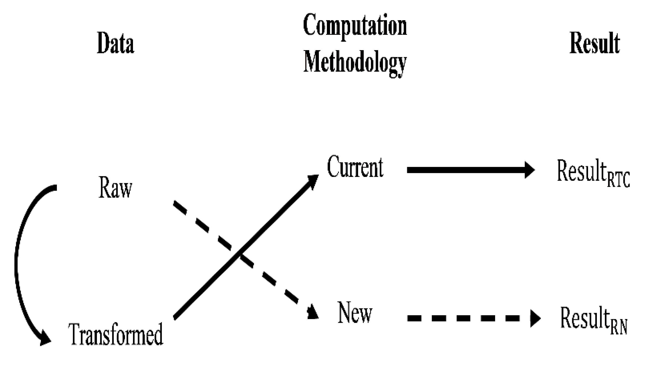
| Figure 3 (dashed path) | Used Data | Raw GORT and SSD | |
| Methodology | No impact of the preceding trial on the current trial | ||
| Distribution | Ex-Gaussian | ||
| Figure 3 (solid path) | Used Data | Estimated state-space GORT and SSD | |
| Methodology | Impact of the preceding trial on the current trial | ||
| Distribution | Lognormal/Normal |
| Inhibition Type | Index Disparities | Mean (95%CI) | t | Sig. (2-Tailed) |
|---|---|---|---|---|
| Proactive | 71.6 (51.4, 91.8) | 7.2 | <0.0001 | |
| Reactive | −10.3 (−20.6, 0.0) | −2.0 | ||
| Reactive | −19.1 (−39.6, −1.5) | −1.9 | ||
| Reactive | 8.8 (−20.1, 37.7) | 0.6 | 0.5 * |
| (a) Measurement Comparisons | |||||
| Measurement | Population | Distribution | Mean (95%CI) | t | Sig. (2-Tailed) |
| Overall | Lognormal | 13.1 (8.4, 17.6) | 5.7 | <0.0001 | |
| Normal | 21.9 (17.4, 26.3) | 9.9 | <0.0001 | ||
| Overall | Lognormal | −0.6 (−9.8, 8.7) | −0.1 | 0.9 | |
| Normal | 8.3 (0.2, 16.4) | 2.1 | 0.04 | ||
| Overall | Lognormal | −1.2 (−8.4, 6.0) | −0.3 | 0.7 | |
| Normal | 7.7 (1.3, 14.1) | 2.4 | 0.02 | ||
| (b) Differential Impact | |||||
| Measurement | Population | SST Distribution | Mean (95%CI) | t | Sig. (2-tailed) |
| ADHD vs. Control | Lognormal | 58.6 (3.0, 114.2) | 2.3 | 0.04 | |
| Normal | 58.8 (1.8, 115.6) | 2.3 | 0.04 | ||
| Ex-Gaussian | 66.5 (10.5, 122.5) | 2.6 | 0.02 | ||
| Ex-Gaussian | 65.6 (5.4, 125.9) | 2.4 | 0.04 | ||
| Ex-Gaussian | 62.3 (5.1, 119.5) | 2.4 | 0.04 | ||
| Pair | N(#SST) | m (#stop) | Mean (95%CI) | t | Sig. (2-Tailed) |
|---|---|---|---|---|---|
| 8.1 | <0.0001 | ||||
| 96 | 24 | 8.5 | <0.0001 | ||
| 4.0 | <0.0001 | ||||
| 10.2 | <0.0001 | ||||
| 192 | 48 | 10.4 | <0.0001 | ||
| 4.2 | <0.0001 | ||||
| 10.4 | <0.0001 | ||||
| 288 | 72 | 10.6 | <0.0001 | ||
| 4.9 | <0.0001 | ||||
| 11.4 | <0.0001 | ||||
| 384 | 96 | 11.1 | <0.0001 | ||
| 5.0 | <0.0001 | ||||
| 11.4 | <0.0001 | ||||
| 480 | 120 | 11.3 | <0.0001 | ||
| 4.8 | <0.0001 | ||||
| 11.8 | <0.0001 | ||||
| 960 | 240 | 11.7 | <0.0001 | ||
| 5.4 | <0.0001 |
© 2020 by the authors. Licensee MDPI, Basel, Switzerland. This article is an open access article distributed under the terms and conditions of the Creative Commons Attribution (CC BY) license (http://creativecommons.org/licenses/by/4.0/).
Share and Cite
Soltanifar, M.; Knight, K.; Dupuis, A.; Schachar, R.; Escobar, M. A Time Series-Based Point Estimation of Stop Signal Reaction Times: More Evidence on the Role of Reactive Inhibition-Proactive Inhibition Interplay on the SSRT Estimations. Brain Sci. 2020, 10, 598. https://doi.org/10.3390/brainsci10090598
Soltanifar M, Knight K, Dupuis A, Schachar R, Escobar M. A Time Series-Based Point Estimation of Stop Signal Reaction Times: More Evidence on the Role of Reactive Inhibition-Proactive Inhibition Interplay on the SSRT Estimations. Brain Sciences. 2020; 10(9):598. https://doi.org/10.3390/brainsci10090598
Chicago/Turabian StyleSoltanifar, Mohsen, Keith Knight, Annie Dupuis, Russell Schachar, and Michael Escobar. 2020. "A Time Series-Based Point Estimation of Stop Signal Reaction Times: More Evidence on the Role of Reactive Inhibition-Proactive Inhibition Interplay on the SSRT Estimations" Brain Sciences 10, no. 9: 598. https://doi.org/10.3390/brainsci10090598
APA StyleSoltanifar, M., Knight, K., Dupuis, A., Schachar, R., & Escobar, M. (2020). A Time Series-Based Point Estimation of Stop Signal Reaction Times: More Evidence on the Role of Reactive Inhibition-Proactive Inhibition Interplay on the SSRT Estimations. Brain Sciences, 10(9), 598. https://doi.org/10.3390/brainsci10090598