Addressing Complete New Item Cold-Start Recommendation: A Niche Item-Based Collaborative Filtering via Interrelationship Mining

Abstract

Recommender system (RS) can be used to provide personalized recommendations based on the different tastes of users. Item-based collaborative filtering (IBCF) has been successfully applied to modern RSs because of its excellent performance, but it is susceptible to the new item cold-start problem, especially when a new item has no rating records (complete new item cold-start). Motivated by this, we propose a niche approach which applies interrelationship mining into IBCF in this paper. The proposed approach utilizes interrelationship mining to extract new binary relations between each pair of item attributes, and constructs interrelated attributes to rich the available information on a new item. Further, similarity, computed using interrelated attributes, can reflect characteristics between new items and others more accurately. Some significant properties, as well as the usage of interrelated attributes, are provided in detail. Experimental results obtained suggest that the proposed approach can effectively solve the complete new item cold-start problem of IBCF and can be used to provide new item recommendations with satisfactory accuracy and diversity in modern RSs.

1. Introduction

With the rapid development of the Internet, data and information are being generated at an unprecedented rate. People cannot acquire useful information quickly and accurately from the huge amount of data around them. Further, the recommender system (RS) can provide personalized items for various types of users, and help users get useful information from large amounts of data. Hence, RSs have great commercial values and research potential and play a significant role in many practical applications and services [1,2,3,4,5,6].

Collaborative filtering (CF) is one of the most successful approaches often used in implementing RSs [7,8,9,10]. Item-based CF (IBCF) approach is a type of CF which supposes that an item will be preferred by a user if the item is similar to the one preferred by the user in the past [11]. IBCF is efficient and easy to implement and has good scalability, hence, it is widely applied in modern RSs, e.g., Amazon and Netflix [12]. One of the main problems of IBCF is the new item cold-start (NICS) problem [12,13,14,15]. NICS is very common in practical RSs, i.e., hundreds of new items are introduced in modern RSs every day. Generally, NICS can be divided into complete new item cold-start (CNICS) where no rating record is available (e.g., i₅ and i₆ in Table 1), and incomplete new item cold-start (INICS) where only a small number of rating records are available (e.g., i₃ and i₄ in Table 1). In this paper, we focus on the problem of producing effective recommendations for new items with no ratings, i.e., CNICS problem. Traditional IBCF suffers from CNICS problem as it relies on previous ratings of the users. In addition, to generate effective recommendations, traditional IBCF requires that items are rated by a sufficient number of users.

Table 1. Illustration of different types of items in RSs.

	u1	u2	u3	u4	u5	u6	u7	…
i1	3	2	3	5	2	2	3	…
i2	4	1	4	2	3	1	5	…
i3	2	1	*	*	*	*	*	…
i4	4	5	1	3	*	*	*	…
i5	*	*	*	*	*	*	*	…
i6	*	*	*	*	*	*	*	…

To solve CNICS problem of IBCF, a simple approach is to randomly present new items to the users in order to gather rating information about those new items. However, this approach tends to achieve low accuracy. On the other hand, additional information about items such as item profiles, tags, and keywords are used in related effective approaches [15,16,17,18,19,20,21,22,23,24]. However, some special additional information is often incomplete or unavailable. In addition, items in practical RSs often have a low amount of profile information (e.g., item attributes), but specific features of new items are difficult to be extracted using limited additional information. Therefore, researchers face difficulty in utilizing only easily obtained and a limited number of additional information in solving the CNICS problem of IBCF.

In this paper, we propose a niche approach which applies interrelationship mining theory to the IBCF approach in order to address the CNICS problem of IBCF. Figure 1 indicates the flow chart of the proposed approach. The proposed approach utilizes interrelationship mining technique to extract new binary relations between item attributes and subsequently construct interrelated attributes according to the original item-attribute matrix. Afterward, the similarity of items is computed with respect to the interrelated attribute information. Next, items with the highest similarity will be selected to comprise the neighborhood of a new item, and rating information of the neighborhood will be used to predict rating score for the new item. Finally, items with the highest predicted rating scores will be recommended to a target user. Experimental results obtained show that our new approach can ameliorate the CNICS problem, and present new item recommendation with better accuracy and diversity at the same time. The academic contributions of this paper can be summarized as follows:

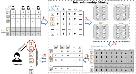
Figure 1. The flow chart of proposed approach. Our approach comprises the following main phases: ① extract item attribute matrix; ② construct interrelated attributes by extending the given binary relations between each pair of attributes; ③ form item interrelated attribute matrix; ④ compute item-item similarity; ⑤ predict rating scores and recommend top N items to the target user.

• Different from related approaches that need special information which is often difficult to obtain [15,16,17,18,19,20,21,22,23,24], the proposed approach can only utilize easily accessible and a limited number of additional information (e.g., item attributes) in solving the CNICS problem of IBCF.
• Different from current related approaches that only utilize attribute values [15,16,17,18,19,20,21,22,23,24], the proposed approach extends the binary relations between each pair of attributes using interrelationship mining and extracts new binary relations to construct interrelated attributes that can reflect the interrelationship between each pair of attributes. Furthermore, some significant properties of interrelated attributes are presented, and theorems for the number of interrelated attributes as well as a detailed process of proof are given in this paper.
• Unlike most related works that can enhance either accuracy or diversity of recommendations, but not in both [15,16,17,18,19,20,21,22,23,24], the proposed approach can provide new item recommendations with satisfactory accuracy and diversity simultaneously, and the experimental results in Section 4 confirm this.

The remaining part of this paper is organized as follows. In Section 2, we introduce the basic idea of IBCF and the associated CNICS problem; interrelationship mining theory is also discussed in this section. In Section 3, we present the proposed approach and discuss its construction and the number of interrelated attributes. In Section 4, we present the experimental setup and an analysis of the experimental results. Finally, we present the conclusion of the paper and suggestion for the future work in Section 5.

2. Background and Related Work

In this section, we introduce the traditional IBCF approach, CNICS problem suffered by IBCF, and the interrelationship mining theory.

2.1. Traditional IBCF Approach and the Associated CNICS Problem

First, we discuss some RS-related notations used in this paper. Given an RS, let $U$ and $I$ be finite sets of users and items, respectively. $R\cup \{\ast \}$ denotes the set of possible item rating scores, the absence of a rating is indicated by an asterisk ($\ast$). The rating score of a user $u\in U$ for item $i\in I$ is denoted by $r_{u,i}\in R\cup \{\ast \}$. $\theta$ is set as the threshold for rating scores, and items with $r_{u,i}\ge \theta$ are regarded as items that are relevant to a user u. Item attribute set is defined as $AT=\left\{a{t}_1,a{t}_2,\dots ,a{t}_l\right\}$, and $AV=\left\{a{v}_1,a{v}_2,\dots ,a{v}_l\right\}$ refers to a set of attribute values, where l is the number of attributes, and $a{t}_l\left(x\right)=a{v}_l\left(x\right)$ means that the value of attribute $a{t}_l$ on item $i_x$ is $a{v}_l$.

The IBCF approach was first proposed by Sarwar [7]. It is one of the most successful approaches and has been employed in famous online marts such as Amazon Inc. To predict the rating score for the target item $i_{ti}$ in which the target user $u_{tu}$ has not rated, first, the IBCF computes similarity between target item $i_{ti}$ and all other items to identify the neighborhood that has most similar items. Afterward, a rating score is computed for target item $i_{ti}$ using the ratings of the neighborhood made by the target user $u_{tu}$ (Equation (1)).

$$P_{tu,ti}=\frac{{{\displaystyle \sum }}_{q\in N_{ti}\left(L\right)\cap I_{tu}}Sim\left(ti,q\right)\ast r_{tu,q}}{{{\displaystyle \sum }}_{q\in N_{ti}\left(L\right)\cap I_{tu}}\left|Sim\left(ti,q\right)\right|}.$$

(1)

Here, $P_{tu,ti}$ denotes the predicted rating made by the target user $u_{tu}$ for the target item $i_{ti}$, $I_{tu}=\{i_x\in I|r_{tu,x}\ne \ast \}$ represents the set of items rated by target user $u_{tu}$, $N_{ti}\left(L\right)$ denotes the neighborhood of the target item $i_{ti}$ comprising most L similar items. Sim(ti,q) denotes the similarity value between target item $i_{ti}$ and item $i_q$. After predicting the rating score for each un-rated item of the target user $u_{tu}$. IBCF sorts all un-rated items in descending order with respect to the predicted rating scores, and the top N items are selected as recommendation for target user $u_{tu}$.

To obtain recommendations with satisfactory accuracy and diversity, the classical IBCF approach requires sufficient number of ratings from users on items [7]; however, if a new item just enters into the RSs, because it has not yet been evaluated by any user, it is crucial for the classical IBCF approach to produce high-quality recommendations for the new item, i.e., the traditional IBCF is susceptible to the CNICS problem. Presently, many approaches have been presented for solving the CNICS problem of IBCF. Gantner et al. [21] presented a framework for mapping item attributes to latent features of a matrix factorization model. The framework is applicable to both user and item attributes and can handle both binary and real-valued attributes. Kula [22] proposed a hybrid matrix factorization model which represents users and items as linear combinations of their content features’ latent factors. Mantrach et al. [23] proposed a matrix factorization model that exploits items’ properties and past user preferences while enforcing the manifold structure exhibited by the collective embedding. Sahoo et al. [24] showed that after forming a good/bad impression on one attribute of items, users will apply this impression to other items, so, item attribute information is often used to compute similarity among items. Herein, we give Jaccard (JAC), a simple and effective similarity measure which uses attribute information to ameliorate the CNICS problem of IBCF [18]:

$$Sim\left(x,y\right)=\frac{\overrightarrow{AV\left(x\right)}\ast \overrightarrow{AV\left(y\right)}}{{\Vert \overrightarrow{AV\left(x\right)}\Vert }^2+{\Vert \overrightarrow{AV\left(y\right)}\Vert }^2-\overrightarrow{AV\left(x\right)}\ast \overrightarrow{AV\left(y\right)}},$$

(2)

where $\overrightarrow{AV\left(x\right)}=\left\{a{v}_1\left(x\right),a{v}_2\left(x\right),\dots ,a{v}_l\left(x\right)\right\}$ is a vector which denotes attributes that item $i_x$ owns. However, these approaches only utilize attribute value of items without considering the hidden information between the given attributes. Furthermore, it is hard to dig out reliable features of new items with a limited number of attributes.

2.2. Interrelationship Mining Theory

Interrelationship mining, an extension of rough set-based data mining, was first proposed by Kudo et al [25]. It extends the domain of comparison of attributes from a value set, $A{V}_a$ of attribute $a$ of the Cartesian product $A{V}_a\times A{V}_b$ with another attribute b, and makes it possible to extract features with respect to a comparison of values of two different attributes. Herein, we provide some brief definitions and refer interested reader to [26,27,28] for more information about interrelationship mining.

Let $a,b\in AT$ be any attributes of a given information table, and $R\subseteq A{V}_a\times A{V}_b$ be any binary relations. We recall that attributes a and b are interrelated by R if and only if there exists an item $i_x\in I$ such that ($\rho \left(x,a\right),\rho \left(x,b\right))\in R$ holds, where $\rho \left(x,a\right)$ denotes the value of item $i_x$ at the attribute a. We denote the set of objects that those values of attributes a and b that satisfy the relation R as follows:

$$R\left(a,b\right)\triangleq \{i_x\in I|\rho \left(x,a\right),\rho \left(x,b\right))\in R\},$$

(3)

and we call the set $R\left(a,b\right)$ the support set of the interrelation between a and b by R.

To evaluate interrelationships between different attributes, Kudo et al. [23] proposed an approach for constructing new binary relation by using given binary relations between values of different attributes. In an information table, the new binary relation set ${\mathcal{R}}_{int}$ for performing interrelationship mining with respect to a given binary relation set ${\mathcal{R}}_{AT}$ can be defined as follows:

$${\mathcal{R}}_{int}={\mathcal{R}}_{AT}\cup \left\{\left\{R_{a_i\times b_i}\right\}|\exists a_i,b_i\in AT\right\}\cup \left\{\{=\}|\mathrm{For}\mathrm{each}aRb\right\},$$

(4)

where each family $\left\{R_{a_i\times b_i}\right\}=\left\{R_{a_i\times b_i}^1,\dots ,R_{a_i\times b_i}^{n_i}\right\}$ consists of $n_i\left(n_i\ge 0\right)$ binary relation(s) defined on $A{V}_{a_i}\times A{V}_{b_i}$. The symbol aRb denotes the interrelated attribute of attributes a and b by the binary relation $R\subseteq A{V}_a\times A{V}_b$.

It is worthy of note that the new binary relation set can not only include equality relation but also other binary relations such that “the value of attribute a is higher/lower than the value of attribute b”.

3. Proposed Approach: IBCF Approach based on Interrelationship Mining

In this section, we would first present the motivation of our proposed approach. Afterward, we introduce a method of constructing interrelated attributes and some significant properties of interrelated attributes. Next, we discuss the use of interrelated attributes based on JAC measure. Finally, we present an instance of how the proposed approach can be used.

3.1. Motivation of the Proposed Approach

To ameliorate the CNICS problem of IBCF, the proposed approach aims to extract more information from limited item attributes of a new item and utilizes the extracted information in selecting a more appropriate neighborhood for a new item in IBCF. This helps to ensure that new item recommendations can be more accurate and diverse.

For a new item, which often has no ratings, existing approaches can be used to restrictedly compare attribute values of the same attribute; however, they do not consider the interrelationship between different attributes. Therefore, it is difficult to extract the following characteristics that are based on a comparison of attribute values between different attributes using the existing approaches:

• A user prefers attribute a of movies more than attribute b,
• The significance of attribute a is identical to the attribute b.

Therefore, the domain of comparison of attribute values needs to be extended so that the values of different attributes can be compared. Hence, we can describe the interrelationships between attributes by a comparison between attribute values of different attributes, and the interrelated attributes can be constructed to incorporate available information of a new item.

3.2. Construction of Interrelated Attributes

First, based on Yao et al. [29], we define the item attribute information table AM in RSs as

$$AM=\left(I,AT,\left\{A{V}_a|a\in AT\right\},{\mathcal{R}}_{AT},\rho \right).$$

(5)

Where I denotes the set of items, AT denotes the set of items’ attributes, $A{V}_a$ denotes the set of attribute values for $a\in AT$, and ${\mathcal{R}}_{AT}=\left\{\left\{R_a\right\}\right|a\in AT\}$ denotes a set of binary relation $\left\{R_a\right\}$ defined on each $A{V}_a$. $\rho$ denotes an information function $\rho :U\times AT\to AV$ that yields a value $\rho \left(x,a\right)\in A{V}_a$ of the attribute $a\in AT$ for each item $i_x\in I$. $AV={\cup }_{a\in AT}A{V}_a$ denotes a set of all attributes’ values in AT. For each item $i_x\in I$ and each attribute $a\in AT$, we assume that the value $\rho \left(x,a\right)$ is either 1 or 0, and say that item $i_x$ owns $a$ if $\rho \left(x,a\right)=1$ holds. The proposed approach is an extension of the existing binary relation set ${\mathcal{R}}_{AT}$ to a new binary relation set ${\mathcal{R}}_{int}$ by using interrelationship mining, with the interrelated attributes constructed to include the available information of a new item. A detailed description of the procedure is presented as follows:

Generally, in RSs, every set of binary relation $\left\{R_a\right\}$ is supposed to be comprised of only the equality relation = on $A{V}_a$, e.g., an item has an attribute a or not. In this case, the characteristic of different attributes is not considered. Thus, to extract the characteristic between different attributes using the given binary relations ${\mathcal{R}}_{AT}$, the extended binary relations ${\mathcal{R}}_{int}$ can be defined as:

$${\mathcal{R}}_{int}={\mathcal{R}}_{AT}\cup \left\{\{=\}|\mathrm{For}\mathrm{each}{a}_{i}R{a}_j\right\}\cup \left\{\left\{R_{a_i\times a_j}\right\}\right|\exists a_i,a_j\in AT\},$$

(6)

where $\left\{R_{a_i\times a_j}\right\}=\left\{R_{a_i\times a_j}^1,\dots ,R_{a_i\times a_j}^{n_i}\right\}$ refers to the new binary relation set for attribute values of $a_i$ and $a_j$. Theoretically, the number of new binary relation can be unlimited. Based on extended binary relations, the interrelated attribute set $A{T}_{int}$ can be expressed as:

$$A{T}_{int}=\left\{a_{i}R{a}_j\right|\exists R\in \left\{R_{a_i\times a_j}\right\},R\left(a_i,a_j\right)\ne \varnothing \},$$

(7)

Further, we explore three types of the binary relation $\left\{{<}_{le},{=}_{eq},{>}_{mo}\right\}$ for each pair of attributes $a_i,a_j\in AT$, and the values of three newly defined interrelated attributes $a_i{<}_{le}{a}_j$, $a_i{=}_{eq}{a}_j$, and $a_i{>}_{mo}{a}_j$ are defined as follows:

$${\rho }_{int}\left(x,a_i{<}_{le}{a}_j\right)=\{\begin{array}{c}1,\rho \left(x,a_i\right)<\rho \left(x,a_j\right),\\ 0,\rho \left(x,a_i\right)\ge \rho \left(x,a_j\right).\end{array}$$

(8)

$${\rho }_{int}\left(x,a_i{=}_{eq}{a}_j\right)=\{\begin{array}{c}1,\rho \left(x,a_i\right)=\rho \left(x,a_j\right)=1,\\ 0,\mathrm{otherwise}.\end{array}$$

(9)

$${\rho }_{int}\left(x,a_i{>}_{mo}{a}_j\right)=\{\begin{array}{c}1,\rho \left(x,a_i\right)>\rho \left(x,a_j\right),\\ 0,\rho \left(x,a_i\right)\le \rho \left(x,a_j\right).\end{array}$$

(10)

In this paper, we consider the interrelated attributes $a_{i}R{a}_j$ of $a_i$ and $a_j$ if and only if $i<j$ holds. From Equations (8)–(10), we discover that ${\rho }_{int}\left(x,a_i{<}_{le}{a}_j\right)=1$ implies that item $i_x$ has attribute $a_j$, but does not have attribute $a_i$; ${\rho }_{int}\left(x,a_i{=}_{eq}{a}_j\right)=1$ implies that item $i_x$ owns both attribute $a_i$ and attribute $a_j$; and ${\rho }_{int}\left(x,a_i{>}_{mo}{a}_j\right)=1$ implies that item $i_x$ owns attribute $a_i$, but does not own attribute $a_j$.

3.3. Number of Interrelated Attributes

In this subsection, we discuss the number of interrelated attributes constructed in the proposed approach.

The proposed approach has an assumption: the interrelated attributes constructed from AT depend on the order of attributes. For any two attributes $a_i,a_j\in AT$ and any binary relation $R\in \left\{{<}_{le},{=}_{eq},{>}_{mo}\right\}$, the index i of $a_i$ must be smaller than the index j of $a_j$ in order to be able to construct the interrelated attributes $a_{i}R{a}_j$. Hence, if we exchange the order of attributes $a_i$ and $a_j$, interrelated attributes $a_{i}R{a}_{i+1}$, …, $a_{i}R{a}_j$ and $a_{i+1}R{a}_j$, …, $a_{j-1}R{a}_j$ are lost and $a_{j}R{a}_{i+1}$, …, $a_{j}R{a}_{j-1}$ and $a_{j}R{a}_i$ and $a_{i+1}R{a}_i$, …, $a_{j-1}R{a}_i$ are newly obtained.

Then, even though the order of the attributes $a_i$ and $a_j$ is exchanged, the number of interrelated attributes that have the value 1 does not change. It is based on the following property.

Lemma 1.

Let $a_i,a_j\in AT$ be any two attributes in which $i<$ j holds, and $i_x\in I$ be an arbitrary item. If the order of the attributes $a_i$ and $a_j$ is changed, there is no change in the number of interrelated attributes that the item $i_x$ owns.

Proof. 

Let $AT=\left\{a_1,\dots ,a_l\right\}$ be a set of attributes that comprises l attribute. Suppose the order of the attributes $a_i$ and $a_j$ is changed, i.e., the order $a_1$, …, $a_{i-1}$, $a_i$, $a_{i+1}$, …, $a_{j-1}$, $a_j$, $a_{j+1}$, …, $a_l$ is changed to $a_1$, …, $a_{i-1}$, $a_j$, $a_{i+1}$, …, $a_{j-1}$, $a_i$, $a_{j+1}$, …, $a_l$. It is obvious that there is no influence of change between $a_i$ and $a_j$ in the case of $\rho \left(x,a_i\right)=\rho \left(x,a_j\right)=1$ or $\rho \left(x,a_i\right)=\rho \left(x,a_j\right)=0$. Further, suppose $\rho \left(x,a_i\right)=1$ and $\rho \left(x,a_j\right)=0$ holds. Then, before changing the order of $a_i$ and $a_j$, it implies that for any attribute $a_k(i<k<j)$, the following three statements can easily be confirmed:

$$\begin{array}{c}{\rho }_{int}\left(x,a_i{=}_{eq}{a}_k\right)=1iff\rho \left(x,a_k\right)=1,\\ {\rho }_{int}\left(x,a_i{>}_{mo}{a}_k\right)=1iff\rho \left(x,a_k\right)=0,\\ {\rho }_{int}\left(x,a_k{>}_{mo}{a}_j\right)=1iff\rho \left(x,a_k\right)=1.\end{array}$$

Hence, if $\rho \left(x,a_k\right)=1$ holds, item $i_x$ owns two interrelated attributes $a_i{=}_{eq}{a}_k$ and $a_k{>}_{mo}{a}_j$. Otherwise, item $i_x$ owns one interrelated attributes $a_i{>}_{mo}{a}_k$. After changing the order of $a_i$ and $a_j$, the following three expressions are obtained:

$$\begin{array}{c}{\rho }_{int}\left(x,a_k{=}_{eq}{a}_i\right)=1iff\rho \left(x,a_k\right)=1,\\ {\rho }_{int}\left(x,a_k{<}_{le}{a}_i\right)=1iff\rho \left(x,a_k\right)=0,\\ {\rho }_{int}\left(x,a_j{<}_{le}{a}_k\right)=1iff\rho \left(x,a_k\right)=1.\end{array}$$

Therefore, by changing the order of $a_i$ and $a_j$, if $\rho \left(x,a_k\right)=1$ holds, the two interrelated attributes $a_i{=}_{eq}{a}_k$ and $a_k{>}_{mo}{a}_j$ are lost, however, item $i_x$ owns two the newly obtained interrelated attributes $a_k{=}_{eq}{a}_i$ and $a_j{<}_{le}{a}_k$. Otherwise, if $\rho \left(x,a_k\right)=0$ holds, the interrelated attribute $a_i{>}_{mo}{a}_k$ is lost, and item $i_x$ owns a new interrelated attribute $a_k{<}_{le}{a}_i$. This implies that changing the order of $a_i$ and $a_j$ does not change the number of interrelated attributes that have a value of 1 in the case of $\rho \left(x,a_i\right)=1$ and $\rho \left(x,a_j\right)=0$. Similarly, another case of $\rho \left(x,a_i\right)=0$ and $\rho \left(x,a_j\right)=1$ can be proven. □

Based on this lemma, the order of attributes can be freely changed without changing the number of interrelated attributes from the original situation. So, without loss of generality, the following situation can be assumed; let $i_x\in I$ be an item. There are l attributes in AT and there is a number $m(1<m<l)$ such that $\rho \left(x,a_1\right)$=…=$\rho \left(x,a_m\right)$= 1 and $\rho \left(x,a_{m+1}\right)$=…=$\rho \left(x,a_l\right)$= 0 hold, respectively. In other words, the item $i_x$ has all m attributes $a_1$, …, $a_m$ and does not have any l - m attributes $a_{m+1}$, …,$a_l$.

In this situation, the number of interrelated attributes with a value of 1 can easily be obtained. Thus, for every two attributes $a_i$,$a_j(1\le i<j\le m)$, it is clear that the value of $a_i{=}_{eq}{a}_j$ is 1 but the values of $a_i{>}_{mo}{a}_j$ and $a_i{<}_{le}{a}_j$ are 0. It can also be easily verified that the number of the interrelated attributes $a_i{=}_{eq}{a}_j$ is $C_m^2$. Similarly, for every two attributes $a_p$, $a_q\left(1\le p\le m\mathrm{and}m+1\le q\le l\right)$, it is also clear that the value $a_p{>}_{mo}{a}_q$ is 1 but $a_p{=}_{eq}{a}_q$ and $a_p{<}_{le}{a}_q$ are 0, hence, the number of interrelated attributes $a_p{>}_{mo}{a}_q$ is $m\times \left(l-m\right)$. These results conclude the following theorem about the number of interrelated attributes with the value 1.

Theorem 1.

Let AT be a set of attributes that comprises l attributes and $i_x\in I$ be an item that owns m attributes in AT. The number of interrelated attributes that item $i_x$ owns, denoted by num(x, l, m), can be obtained using

$$num\left(x;l,m\right)=C_m^2+m\left(l-m\right).$$

(11)

3.4. JAC based on Interrelated Attributes

In this subsection, we employ JAC measure (Equation (2)) to introduce the application of the interrelated attributes between two items and the number of interrelated attributes that each item owns. Note that the interrelated attributes can also be applied to other approaches which utilize item attributes in generating recommendations.

Let AT be the set of attributes that comprises l attributes and $i_x,i_y\in I$ be any two items. Suppose item $i_x$ owns $m_x$ attributes and item $i_y$ owns $m_y$ attributes, respectively. By changing the order of attributes freely with respect to Lemma 1, without loss of generality, the following condition can be assumed:

• Both items $i_x$ and $i_y$ have $n_1\left(n_1\ge 0\right)$ attributes $a_1,\dots ,a_{n_1}$.
• Item $i_x$ also has all $n_2\left(n_2\ge 0\right)$ attributes $b_1,\dots ,b_{n_2}$ but item $i_y$ does not have any of these attributes.
• Item $i_y$ also has all $n_3\left(n_3\ge 0\right)$ attributes $c_1,\dots ,c_{n_3}$ but item $i_x$ does not have any of these attributes.
• Both items $i_x$ and $i_y$ do not have $n_4\left(n_4\ge 0\right)$ attributes $d_1,\dots ,d_{n_4}$,

where, the conditions of the number of attributes that item $i_x$ and $i_y$ own, $n_1+n_2+n_3+n_4=l$, $n_1+n_2=m_x$, and $n_1+n_3=m_y$ hold, respectively.

Using Theorem 1, the number of interrelated attributes that item $i_x$ owns can be obtained as follows:

$$\begin{array}{ll}num\left(x;l,m_x\right)& =C_{m_x}^2+m_x\left(l-m_x\right)\\ & =C_{n_1+n_2}^2+(n_1+n_2)(n_3+n_4)\\ & =C_{n_1+n_2}^2+n_1{n}_4+n_1{n}_3+n_2{n}_3+n_2{n}_4\end{array}$$

(12)

Similarly, the number of interrelated attributes that item $i_y$ owns is

$$num\left(y;l,m_y\right)=C_{n_1+n_3}^2+n_1{n}_4+n_1{n}_2+n_2{n}_3+n_3{n}_4$$

(13)

Because both items $i_x$ and $i_y$ have $n_1\left(n_1\ge 0\right)$ attributes $a_1,\dots ,a_{n_1}$, either there is no interrelated attribute $a_i{=}_{eq}{a}_j(1\le i<j\le n_1)$ when $n_1=0$ or $n_1=1$, or there is $C_{n_1}^2$ attributes $a_i{=}_{eq}{a}_j(n_1\ge 2\mathrm{and}1\le i<j\le n_1)$ that both items $i_x$ and $i_y$ own commonly. Hence, in the case of item $i_x$, the rest $C_{n_1+n_2}^2-C_{n_1}^2$ interrelated attributes based on the relation ${=}_{eq}$ are owned by only item $i_x$ and not item $i_y$. Similarly, in the case of item $i_y$, $C_{n_1+n_3}^2-C_{n_1}^2$ interrelated attributes based on the relation ${=}_{eq}$ are owned by only item $i_y$ and not item $i_x$.

Moreover, similar to the above discussion, both item $i_x$ and item $i_y$ do not have $n_4\left(n_4\ge 0\right)$ attributes $d_1,\dots ,d_{n_4}$, either because there is no interrelated attribute $a_i{>}_{mo}{d}_q\left(1\le i\le n_1\mathrm{and}1\le q\le n_4\right)$ if when $n_1=0$ or $n_4=0$ or $n_1{n}_4$ interrelated attributes $a_i{>}_{mo}{d}_q$ that item $i_x$ and item $i_y$ own commonly. Based on the structure of attributes that item $i_x$ and item $i_y$ own, it is obvious that the remaining interrelated attributes denoted by ${>}_{mo}$ (or ${<}_{le}$) are owned by either item $i_x$ or item $i_y$ only.

These discussions conclude the following results about the relationship between JAC similarity between item $i_x$ and item $i_y$ and the number of interrelated attributes that item $i_x$ and item $i_y$ own commonly.

Theorem 2.

Let AT be a set of attributes that comprises l attributes, item $i_x,i_y\in I$ be any two items and suppose that item $i_x$ owns $m_x$ attributes and item $i_y$ owns $m_y$ attributes, respectively. The JAC similarity Sim(x,y) can be obtained as follows:

$$Sim\left(x,y\right)=\frac{com\left(x,y\right)}{num\left(x;l,m_x\right)+num\left(y;l,m_y\right)-com\left(x,y\right)},$$

(14)

where $com\left(x,y\right)$ is the number of interrelated attributes that item $i_x$ and item $i_y$ own commonly, which is defined as:

$$com\left(x,y\right)=C_{n_1}^2+n_1{n}_4.$$

(15)

It is important that the number $n_4$ of attributes that both item $i_x$ and item $i_y$ do not own is used in Equation (14). This implies that the JAC similarity based on interrelated attributes implicitly evaluates the number of attributes that both items do not own. Because JAC similarity based on the original attributes presented in Equation (2) evaluates only the ratio of commonly owned attributes, attributes that both items do not own are not considered in this case. This shows that it is possible that JAC obtained using interrelated attributes can be used to provide recommendations with high diversity based on the similarity obtained using the commonly owned attributes and attributes that are not commonly owned. It is necessary to conduct further research on this; hence, it would be one of our future works.

3.5. Example of Proposed Approach in CNICS Problem

Herein, we introduce the procedure of the proposed approach in Algorithm 1. Furthermore, we present an example to describe our proposed approach more clearly. Table 2 shows a user-item rating information table about rating scores obtained from four users and seven items; $i_{ti1}$ and $i_{ti2}$ denote the target items and have no ratings from users. The rating value is from 1 to 5, and a higher value indicates that the user likes the given item more. Table 3 shows the item attribute information table about seven items, and three attributes $a{t}_1,a{t}_2,$ and $a{t}_3$ are considered, where a value of 1 indicates that the item has that attribute and a value of 0 means it does not have that attribute. Note that items can be in several attributes simultaneously. Herein, we suppose user $u_4$ is the target user, therefore, we need to predict rating scores of $i_{ti1}$ and $i_{ti2}$ for user $u_4$.

Table 2. Example of user-item rating information table.

	u1	u2	u3	u4
i1	3	2	4	2
i2	5	4	5	4
i3	4	5	1	3
i4	1	3	1	1
i5	2	4	2	5
iti1	*	*	*	*
iti2	*	*	*	*

Table 3. Example of item attribute information table.

	at1	at2	at3
i1	1	0	0
i2	1	1	1
i3	1	0	1
i4	0	0	1
i5	0	1	0
iti1	0	1	1
iti2	1	1	0

Step 1: Construct interrelated attributes. Based on three item attributes $\{a{t}_1,a{t}_2,a{t}_3\}$ shown in Table 3, we extract the relation between each pair of attributes using Equations (8)–(10). Table 4 is the interrelated attribute information table.

Table 4. Example of item interrelated attribute information table.

	at1>leat2	at1>leat2	at1>leat2	at1=eqat2	at1=eqat2	at1=eqat2	at1<moat2	at1<moat2	at1<moat2
i1	1	1	0	0	0	0	0	0	0
i2	0	0	0	1	1	1	0	0	0
i3	1	0	0	0	1	0	0	0	1
i4	0	0	0	0	0	0	0	1	1
i5	0	0	1	0	0	0	1	0	0
iti1	0	0	0	0	0	1	1	1	0
iti2	0	1	1	1	0	0	0	0	0

Step 2: Similarity computation. Based on the information of new interrelated attributes, we employ Equation (14) to compute similarity between each pair of items. Herein, we use the similarity computation of $i_1$ and $i_3$ as an example. From Table 3, according to discussions in Section 3.4, we obtain that the following.

• Both $i_1$ and $i_3$ have $n_1=1$ attribute $a{t}_1$.
• There is no attribute that $i_1$ has but $i_3$ does not have, so $n_2=0$.
• $i_3$ has $n_3=1$ attribute $a{t}_3$ but $i_1$ does not have that.
• Both $i_1$ and $i_3$ do not have $n_4=1$ attribute $a{t}_2$.

Algorithm 1 Proposed approach
Input: User-item matrix RM, item-attribute matrix AM, and a target user $u_{tu}$.
Output: Recommended items for the target user $u_{tu}$.
	$AT$: The set of items’ attributes.
	$A{T}_{int}$: The set of interrelated attributes.
	$N_{ti}\left(L\right)$: Neighborhood of the target item $i_{ti}$.
	L: Number of items in the neighborhood $N_{ti}\left(L\right)$ of the target item $i_{ti}$.
	N: Number of items recommended to the target user $u_{tu}$.
	$I_{tu}^c$: The set of items that the target user $u_{tu}$ has not rated.
	$P_{tu,ti}$: Rating prediction of target item $i_{ti}$ for the target user $u_{tu}$.
1:	$A{T}_{int}=\varnothing$
2:	For each pair of attributes $\left\{a_i,a_j\right\}\subseteq AT(i<j)$ do
3:	Obtain the three interrelated attributers:
	$A{T}_{int}≔A{T}_{int}\cup \left\{a_{i}R{a}_j|R\in \left\{{<}_{le},{=}_{eq},{>}_{mo}\right\}\right\}$
4:	End for
5:	For each interrelated attribute $a_{i}R{a}_j\in A{T}_{int}$ do
6:	For each item $i_x\in I$ do
7:	Set the attribute value $\rho \left(x,a_{i}R{a}_j\right)$ of $i_x$ by Equations (8)–(10)
8:	End for
9:	End for
10:	For each pair of items $\left\{i_m,i_n\right\}\subseteq I$ do
11:	Compute the similarity between $i_m$ and $i_n$ according to interrelated attributes
12:	End for
13:	For each target item $i_{ti}\in I_{tu}^c$ do
14:	Find the L most similar items of target item $i_{ti}$ to comprise neighborhood $N_{ti}\left(L\right)$
15:	Predict rating score $P_{tu,ti}$ of target item $i_{ti}$ from the items in $N_{ti}\left(L\right)$
16:	End for
17:	Recommend the top N target items having the highest predicted rating scores to the target user $u_{tu}$

According to Equations (12) and (13), we can obtain the number of interrelated attributes of $i_1$ and $i_3$, respectively.

$$\begin{array}{c}num\left(i_1;l,m_{i_1}\right)=C_{n_1+n_2}^2+n_1{n}_4+\left(n_1{n}_3+n_2{n}_3+n_2{n}_4\right)=2;\\ num\left(i_3;l,m_{i_3}\right)=C_{n_1+n_3}^2+n_1{n}_4+\left(n_1{n}_2+n_2{n}_3+n_3{n}_4\right)=3;\end{array}$$

Then, according to Equation (15), we can obtain

$$com\left(i_1,i_3\right)=C_{n_1}^2+n_1{n}_4=1.$$

Finally, we can compute the similarity between $i_1$ and $i_3$ as

$$Sim\left(i_1,i_3\right)=\frac{com\left(i_1,i_3\right)}{num\left(i_1;l,m_{i_1}\right)+num\left(i_3;l,m_{i_3}\right)-com\left(i_1,i_3\right)}=0.25.$$

Similarly, we can compute similarity for each other pair of items, and the results of item similarity evaluation are shown in Table 5. For the target items $i_{ti1}$ and $i_{ti2}$, we sort their similar items according to a descending order of the value of similarity. If only three nearest items are considered as a neighborhood, the neighborhood $N_{ti1}\left(3\right)$ and $N_{ti2}\left(3\right)$ of target items $i_{ti1}$ and $i_{ti2}$ are:

$$N_{ti1}\left(3\right)=\left\{i_4,i_5,i_2\right\};N_{ti2}\left(3\right)=\left\{i_1,i_5,i_2\right\}.$$

Table 5. Example of item similarity information table.

	i1	i2	i3	i4	i5	iti1	iti2
i1	1	0	0.25	0	0	0	0.25
i2	0	1	0.20	0	0	0.20	0.20
i3	0.25	0.20	1	0.25	0	0	0
i4	0	0	0.25	1	0	0.25	0
i5	0	0	0	0	1	0.25	0.25
iti1	0	0.20	0	0.25	0.25	1	0
iti2	0.25	0.20	0	0	0.25	0	1

Step 3: Rating prediction. From the rating scores of $N_{ti1}\left(3\right)$ and $N_{ti2}\left(3\right)$, we can use Equation (1) to predict user $u_4$’s rating scores for $i_{ti1}$ and $i_{ti2}$. Here

$$P_{4,ti1}=3.286;P_{4,ti2}=3.643.$$

Step 4: Item recommendations. Because $P_{4,ti1}<P_{4,ti2}$, hence, if we select the top item as a recommendation, item $i_{ti2}$ will be recommended to user $u_4$.

4. Experiments and Evaluation

In this section, we describe the evaluation datasets and measures, examine the performance of the proposed approach, and compare the proposed approach’s effects with the traditional IBCF using different datasets.

4.1. Experimental Setup and the Evaluation Metrics

Here, we used two popular real-world datasets that are often used in evaluating RSs. One is the MovieLens 100K dataset [30], which contains 1,682 movies, 943 users, and a total of 100,000 ratings. The other dataset is the MovieLens 1M dataset that contains a total of 1,000,209 ratings of 3900 movies from 6040 users. In both of the two datasets, the ratings are on a {1, 2, 3, 4, 5} scale, and each user rated at least 20 movies, with each movie having the following attributes: Action, Adventure, Animation, Children’s, Comedy, Crime, Documentary, Drama, Fantasy, Film-Noir, Horror, Musical, Mystery, Romance, Sci-Fi, Thriller, War, and Western.

In the experiment, for each dataset, we randomly selected 20% items as test items, and the remaining 80% items were treated as the training items. To ensure that each item in the test items is a new item which has no rating records, all the ratings in each test item were masked. We utilized ratings of the training items to predict rating scores for the test items, and the test items were used to evaluate the performance of the proposed approach. Note that, in order to avoid the impact of overfitting problem, we repeat the experiments 10 times for each dataset and compute the average values as our experimental results.

To measure the performance of the proposed approach, we used precision and recall metrics to represent the accuracy of the recommendations. In addition, we used mean personality (MP) and mean novelty (MN) to evaluate the diversity of the recommendations. In accordance with Herlocker’s research [31], to maintain real-time performance, we selected different sized L neighborhoods from candidate neighbors, L$\in$ {20, 25, 30, …, 60}. Furthermore, to calculate the precision and recall, we treated items rated not less than three as relevant items, and the number of recommendations was set to 2, 4, 6, and 8.

Precision means the proportion of relevant recommended items from the total number of recommended items for the target user. Further, higher precision values indicate better performance. Suppose that $N_s$ is the number of recommended items for a target user, $N_{rs}$ denotes the number of items the target user likes that appear in the recommended list. The precision metric can be expressed as follows:

$$Precision=\frac{N_{rs}}{N_s}.$$

(16)

Recall indicates the proportion of relevant recommended items from all relevant items for the target user. Similar to precision, higher recall values indicate better performance. Herein, $N_r$ denotes the number of items preferred by the target user. The recall metric can be computed as follows:

$$Recall=\frac{N_{rs}}{N_r}.$$

(17)

MP indicates the average degree of overlap between every two users’ recommendations. For example, for two users $u_i$ and $u_j$, we count the number of recommendations of the corresponding top N items, $Re{c}_i\left(N\right)$ and $Re{c}_j\left(N\right)$, and further normalize this number using the threshold value N to obtain the degree of overlap between two sets of recommendations. It is clear that using an approach of higher recommendation diversity result in larger MP. As suggested by Gan and Jiang in [32], we set N = 20 in calculating this metric.

$$RMP\left(N\right)=1-\frac{1}{N}\frac{2}{\left|U\right|\left(\left|U\right|-1\right)}{\displaystyle \sum }_{1\le i\le j\le \left|U\right|}\left|Re{c}_i\left(N\right)\cap Re{c}_j\left(N\right)\right|,$$

(18)

MN indicates the novelty of recommendations provided to the users. First, it calculates the fraction of users who have ever rated each recommendation, and then computes the sum over all recommendations in $Re{c}_m\left(N\right)$ to obtain the novelty for user $u_m$. Finally, we calculate the average novelty over all users as

$$MN\left(N\right)=-\frac{1}{\left|U\right|}{\displaystyle \sum }_{1\le m\le \left|U\right|}{\displaystyle \sum }_{n\in Re{c}_m\left(N\right)}lo{g}_2{f}_n,$$

(19)

where $f_n$ indicates the fraction of users who rated the n-th item. We also set N = 20 in calculating this metric as suggested in [32], and an approach will have a larger MN if it can be used to make newer recommendations.

4.2. Experimental Results and Analysis

We conducted experiments to evaluate the performance of our proposed approach which applies interrelationship mining to IBCF as IM-IBCF. In addition, we compared the results obtained with that of IBCF. In all the experiments conducted, we employed JAC measure to compute similarity, and weighted sum approach was used to predict the rating scores. Finally, we selected the top N candidate items with highest predicted rating scores as the recommendations.

Table 6 and Table 7 show a comparison of the precision and recall results of the mentioned recommendation approaches on MovieLens 100K dataset. Moreover, the tables also show comparative results for a different number of neighborhoods and recommended items. It should be noted that we grouped experimental data according to the number of recommended items and neighborhoods (e.g., experimental results in N = 2 and L =20 will be a group), the best result of each group is boldfaced, and the best performance among all approaches in each table is underlined. From the results, it is clear that the highest precision and recall results are obtained for different numbers of recommended items and neighborhood. For example, if the number of recommended items is set to 2, the best result of precision measure is 0.500 when the number of neighborhoods is 60, and the best recall value is 0.242 when the number of neighborhood is set to 35. Moreover, when the number of neighborhoods is fixed, values of precision for each mentioned approach decrease as the number of recommended items increases; on the contrary, recall result increases as the number of recommended items increases. In addition, it can be concluded from each table results that precision and recall gain their best results for a different number of recommended items and neighborhood. For example, for the precision metric, the best value was obtained when N = 2 and L = 60; however, the best recall result was obtained when N = 8 and L = 45. According to the results in Table 6 and Table 7, we can conclude that although values of precision and recall of the proposed IM-IBCF approach are worse than the one obtained using IBCF when the number of neighborhoods is less than 45, IM-IBCF approach outperforms IBCF as the number of neighborhood increases. Furthermore, compared with IBCF, IM-IBCF can be used to obtain the best precision and recall results when L = 60, N = 2 and L = 45, N = 8, respectively. Therefore, the proposed IM-IBCF can provide more accurate recommendation than IBCF when used on MovieLens 100K dataset.

Table 6. Results of precision measure on the MovieLens 100K dataset.

#Recommended Items	Recommendation Approach	#Neighborhood
		L = 20	L = 25	L = 30	L = 35	L = 40	L = 45	L = 50	L = 55	L = 60
N = 2	IM-IBCF	0.478	0.479	0.480	0.476	0.473	0.468	0.462	0.473	0.500
	IBCF	0.474	0.524	0.526	0.475	0.417	0.434	0.450	0.447	0.444
N = 4	IM-IBCF	0.261	0.266	0.270	0.274	0.278	0.273	0.270	0.273	0.276
	IBCF	0.273	0.286	0.289	0.255	0.236	0.233	0.237	0.229	0.222
N = 6	IM-IBCF	0.196	0.199	0.209	0.211	0.214	0.207	0.204	0.198	0.191
	IBCF	0.234	0.221	0.222	0.219	0.216	0.201	0.193	0.189	0.186
N = 8	IM-IBCF	0.164	0.197	0.187	0.164	0.203	0.195	0.188	0.186	0.185
	IBCF	0.207	0.166	0.169	0.201	0.161	0.157	0.153	0.147	0.141

Table 7. Results of recall measure on the MovieLens 100K dataset.

#Recommended Items	Recommendation Approach	#Neighborhood
		L = 20	L = 25	L = 30	L = 35	L = 40	L = 45	L = 50	L = 55	L = 60
N = 2	IM-IBCF	0.235	0.238	0.237	0.242	0.239	0.235	0.233	0.236	0.241
	IBCF	0.231	0.239	0.238	0.239	0.240	0.232	0.230	0.232	0.239
N = 4	IM-IBCF	0.251	0.249	0.251	0.258	0.263	0.265	0.261	0.269	0.273
	IBCF	0.246	0.257	0.259	0.262	0.257	0.256	0.254	0.259	0.265
N = 6	IM-IBCF	0.273	0.264	0.271	0.281	0.278	0.279	0.284	0.285	0.289
	IBCF	0.268	0.269	0.279	0.277	0.273	0.280	0.281	0.283	0.287
N = 8	IM-IBCF	0.286	0.283	0.290	0.286	0.297	0.311	0.308	0.307	0.303
	IBCF	0.281	0.287	0.285	0.288	0.290	0.293	0.297	0.304	0.301

Table 8 and Table 9 indicate the precision and recall results with a different number of recommended items and neighborhoods on the MovieLens 1M dataset. According to the results, we can conclude that the proposed IM-IBCF can be used to obtain the best precision results when N = 2 and L = 35. And best performance of the recall metric can also be obtained using the proposed IM-IBCF approach when N = 8 and L = 40. Moreover, it can be concluded that higher precision and recall values among the above mentioned two approaches are obtained for different numbers of recommended items and neighborhood. For example, when the number of recommended items is set to 2 (i.e., N = 2), the highest precision value reported is 0.379 for the IM-IBCF approach when the number of neighborhoods is 35; however, if the number of recommended items is set to 8, the best precision result obtained is 0.191 when the number of neighborhoods is 30 (i.e., L = 30). Similarly, for the recall measure, if the number of neighborhood is set to 20 (i.e., L = 20), the best value 0.178 can be obtained using the IBCF approach when the number of recommended items is 8; however, if the number of neighborhood is 30 (i.e., L = 30), the highest recall result obtained using the proposed IM-IBCF approach is 0.194 when the number of recommended items is set to 8. From Table 6, Table 7, Table 8 and Table 9, we can conclude that, for precision and recall metrics, the proposed IM-IBCF gives higher values than IBCF in both MovieLens 100K and MovieLens 1M datasets. Because higher values indicate better accuracy performance, it implies that the proposed approach can predict rating scores for new items more accurately.

Table 8. Results of precision measure on the MovieLens 1M dataset.

#Recommended Items	Recommendation Approach	#Neighborhood
		L = 20	L = 25	L = 30	L = 35	L = 40	L = 45	L = 50	L = 55	L = 60
N = 2	IM-IBCF	0.374	0.373	0.375	0.379	0.371	0.369	0.367	0.364	0.361
	IBCF	0.372	0.375	0.376	0.374	0.368	0.366	0.364	0.362	0.360
N = 4	IM-IBCF	0.288	0.290	0.293	0.297	0.295	0.291	0.292	0.294	0.296
	IBCF	0.289	0.291	0.287	0.286	0.284	0.282	0.280	0.284	0.288
N = 6	IM-IBCF	0.217	0.216	0.213	0.210	0.218	0.216	0.214	0.211	0.210
	IBCF	0.215	0.218	0.219	0.213	0.213	0.212	0.210	0.207	0.202
N = 8	IM-IBCF	0.186	0.187	0.191	0.187	0.185	0.182	0.181	0.180	0.177
	IBCF	0.182	0.189	0.188	0.185	0.184	0.183	0.180	0.179	0.176

Table 9. Results of recall measure on the MovieLens 1M dataset.

#Recommended Items	Recommendation Approach	#Neighborhood
		L = 20	L = 25	L = 30	L = 35	L = 40	L = 45	L = 50	L = 55	L = 60
N = 2	IM-IBCF	0.128	0.131	0.133	0.130	0.129	0.122	0.118	0.119	0.115
	IBCF	0.089	0.126	0.129	0.132	0.112	0.123	0.115	0.112	0.109
N = 4	IM-IBCF	0.159	0.164	0.165	0.166	0.169	0.158	0.155	0.148	0.142
	IBCF	0.149	0.121	0.122	0.125	0.128	0.131	0.133	0.135	0.136
N = 6	IM-IBCF	0.166	0.169	0.171	0.177	0.181	0.172	0.165	0.157	0.153
	IBCF	0.162	0.166	0.174	0.179	0.171	0.168	0.164	0.156	0.151
N = 8	IM-IBCF	0.176	0.186	0.194	0.203	0.205	0.196	0.191	0.184	0.188
	IBCF	0.178	0.179	0.181	0.183	0.186	0.187	0.189	0.186	0.184

Figure 2 shows the performance of MP and MN for different sizes of neighborhoods on the MovieLens 100K dataset. From the figures, we can observe that increasing the size of the neighborhood would result in higher MP values for both approaches. However, the proposed IM-IBCF produces a better performance than IBCF. For MN metric, the proposed IM-IBCF surpasses IBCF in the whole range of size of neighborhoods. Figure 3 presents comparison of MP and MN results obtained using the MovieLens 1M dataset. As shown in the figures, MP values of IM-IBCF has no remarkable change in the whole size of the neighborhood range; however, IBCF increases clearly as the size of neighborhood increases. However, the proposed IM-IBCF can surpass IBCF over all ranges of neighborhoods. For MN metric, increasing the size of neighborhood results in an increase in MN values of the two approaches. Further, the proposed IM-IBCF approach surpasses IBCF for the whole range of neighborhoods. From Figure 2 and Figure 3, we can conclude that the proposed IM-IBCF approach produces better MP and MN results than the IBCF approach. This implies that a new item’s neighborhood selected using the proposed approach IM-IBCF includes a wider variety of items. Hence, IM-IBCF can provide recommendations with better diversity.

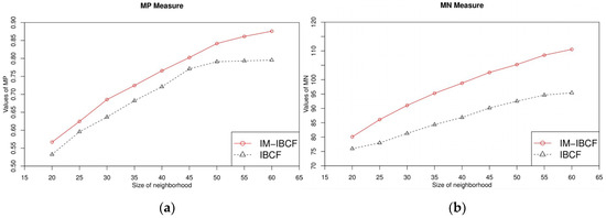
Figure 2. MP (a) and MN (b) results with MovieLens 100K dataset.

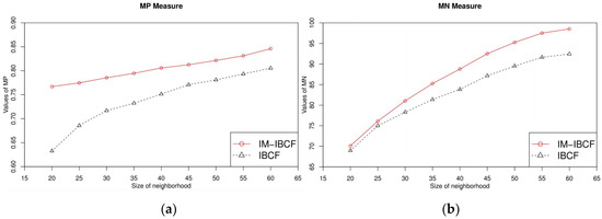
Figure 3. MP (a) and MN (b) results with MovieLens 1M dataset.

Experimental results above show that the proposed approach has better accuracy and diversity than IBCF on the CNICS problem. Because a new item often has no rating records, the IBCF uses JAC measure to compute similarity by comparing attribute values between items, however it cannot explore the hidden information from the given attributes. By extending binary relations between different attributes, the proposed approach constructs interrelated attributes for each item so that more information can be utilized in evaluating the similarity computation. Further, items in a new item’s neighborhood will be more similar to this new item, which shows that the accuracy of the recommendation has improved. Moreover, items with more common attributes will have higher similarity in IBCF, thereby making items in a neighborhood to concentrate on a few types. The proposed approach can be used to extract characteristic from different attributes, which can enhance distinction among different items. Thus, in IM-IBCF, items types in the neighborhood are more than in IBCF, and more types of items can be recommended to the target user. Therefore, the diversity of recommendations has also been enhanced.

5. Conclusions and Future Work

In this paper, we have proposed a new approach for solving the CNICS problem of the IBCF approach, which employs interrelationship mining to increase available information on a new item. First, it extends binary relations between different attributes using the given binary relations. Afterward, it constructs interrelated attributes that can express characteristics between a pair of different attributes by using the new binary relations. Next, interrelated attributes are used to compute similarity, and items with a higher similarity will be selected to be part of the neighborhood of a new item. Finally, the proposed approach uses rating information of the neighborhood to predict rating score, and items with the highest predicted rating scores will be recommended. We evaluated the performance of the proposed approach using not only the accuracy but also the diversity metric. Because more available information can be extracted by performing interrelationship mining (e.g., interrelated attributes) for a new item, the approach achieved significant improvements in both the accuracy and diversity performance. Therefore, the proposed approach can be used in RSs to ameliorate the CNICS problem of IBCF.

The interrelationship mining used in the proposed approach can extend the domain of comparison of different attribute values and make values of different attributes become comparable. But for RSs which have different types of binary relations and attributes, determining the type of binary relation that should be extracted and how many interrelated attributes should be constructed is a challenging issue; hence, we plan to look into this in our future work.

References

- Adomavicius, G.; Tuzhilin, A. Toward the next generation of recommender systems: A survey of the state-of-the-art and possible extensions. IEEE Trans. Knowl. Data Eng. 2005, 17, 734–749. [Google Scholar] [CrossRef]
- Bobadilla, J.; Ortega, F. Recommender system survey. Knowl.-Based Syst. 2013, 46, 109–132. [Google Scholar] [CrossRef]
- Lu, J.; Wu, D.; Mao, M.; Wang, W.; Zhang, W. Recommender system application developments: A survey. Decis. Support Syst. 2015, 74, 12–32. [Google Scholar] [CrossRef]
- Zhang, Z.; Kudo, Y.; Murai, T. Neighbor selection for user-based collaborative filtering using covering-based rough sets. Ann. Oper. Res. 2017, 256, 359–374. [Google Scholar] [CrossRef]
- Rosaci, D. Finding semantic associations in hierarchically structured groups of Web data. Form. Asp. Comput. 2015, 27, 867–884. [Google Scholar] [CrossRef]
- De Meo, P.; Fotia, L.; Messina, F.; Rosaci, D.; Sarné, G.M. Providing recommendations in social networks by integrating local and global reputation. Inf. Syst. 2018, 78, 58–67. [Google Scholar] [CrossRef]
- Sarwar, B.; Karypis, G.; Konstan, J.; Riedl, J. Item-based collaborative filtering recommendation algorithm. In Proceedings of the 10th International Conference on World Wide Web, Hong Kong, China, 1–5 May 2001; pp. 285–295. [Google Scholar]
- Chen, T.; Sun, Y.; Shi, Y.; Hong, L. On sampling strategies for neural network-based collaborative filtering. In Proceedings of the 23th ACM SIGKDD International Conference on Knowledge Discovery and Data Mining, Halifax, NS, Canada, 13–17 August 2017; pp. 767–776. [Google Scholar]
- Thakkar, P.; Varma, K.; Ukani, V.; Mankad, S.; Tanwar, S. Combing user-based and item-based collaborative filtering using machine learning. Inf. Commun. Technol. Intell. Syst. 2019, 107, 173–180. [Google Scholar]
- Guo, G.; Zhang, J.; Yorke-Smith, N. TrustSVD: Collaborative filtering with both the explicit and implicit influence of user trust and of item ratings. In Proceedings of the 29th AAAI Conference on Artificial Intelligence, Texas, TX, USA, 25–30 February 2015; pp. 123–129. [Google Scholar]
- Deshpande, M.; Karypis, G. Item-based top-n recommendation algorithms. ACM Trans. Inf. Syst. 2004, 22, 143–177. [Google Scholar] [CrossRef]
- Lika, B.; Kolomvatsos, K.; Hadjiefthymiades, S. Facing the cold start problem in recommender systems. Expert Syst. Appl. 2014, 41, 2065–2073. [Google Scholar] [CrossRef]
- Wei, J.; He, J.; Chen, K.; Zhou, Y.; Tang, Z. Collaborative filtering and deep learning based recommendation system for cold start items. Expert Syst. Appl. 2017, 69, 29–39. [Google Scholar] [CrossRef]
- Said, A.; Jain, B.J.; Albayrak, S. Analyzing weighting schemes in collaborative filtering: Cold start, post cold start and power users. In Proceedings of the 27th Annual Symposium on Applied Computing, Trento, Italy, 26–30 March 2012; pp. 2035–2040. [Google Scholar]
- Ahn, H.J. A new similarity measure for collaborative filtering to alleviate the new user cold-starting problem. Inf. Sci. 2008, 178, 37–51. [Google Scholar] [CrossRef]
- Basilico, J.; Hofmann, T. Unifying collaborative and content-based filtering. In Proceedings of the 21th International Conference on Machine Learning, Banff, AB, Canada, 4–8 July 2004; pp. 9–26. [Google Scholar]
- Cohen, D.; Aharon, M.; Koren, Y.; Somekh, O.; Nissim, R. Expediting exploration by attribute-to-feature mapping for cold-start recommendations. In Proceedings of the 7th ACM Conference on RecSys, Como, Italy, 27–31 August 2017; pp. 184–192. [Google Scholar]
- Koutrika, G.; Bercovitz, B.; Garcia-Molina, H. FlexRecs: Expressing and combining flexible recommendations. In Proceedings of the ACM SIGMOD International Conference on Management of Data, Providence, RI, USA, 29 June–2 July 2009; pp. 745–758. [Google Scholar]
- Schein, A.I.; Popescul, A.; Ungar, L.H.; Pennock, D.M. Generative models for cold-start recommendations. In Proceedings of the 2001 SIGIR Workshop Recommender Systems, New Orleans, LA, USA, September 2001; Volume 6. [Google Scholar]
- Stern, D.H.; Herbrich, R.; Graepel, T. Matchbox: Large scale online bayesian recommendations. In Proceedings of the 18th International Conference on World Wide Web, Madrid, Spain, 20–24 April 2009; pp. 111–120. [Google Scholar]
- Gantner, Z.; Drumond, L.; Freudenthaler, C.; Rendle, S.; Schmidt-Thieme, L. Learning Attribute-to-Feature Mappings for Cold-Start Recommendations. In Proceedings of the 10th IEEE International Conference on Data Mining, Sydney, Australia, 13–17 December 2010; pp. 176–185. [Google Scholar]
- Kula, M. Metadata embeddings for user and item cold-start recommendations. In Proceedings of the 2nd CBRecSys, Vienna, Austria, 16–20 September 2015; pp. 14–21. [Google Scholar]
- Mantrach, A.; Saveski, M. Item cold-start recommendations: Learning local collective embeddings. In Proceedings of the 8th ACM Conference on RecSys, Foster City, Silicon Valley, CA, USA, 6–10 October 2014; pp. 89–96. [Google Scholar]
- Sahoo, N.; Krishnan, R.; Duncan, G.; Callan, J. The halo effect in multicomponent ratings and its implications for recommender systems: The case of yahoo! movies. Inf. Syst. Res. 2013, 23, 231–246. [Google Scholar] [CrossRef]
- Kudo, Y.; Murai, T. Indiscernibility relations by interrelationships between attributes in rough set data analysis. In Proceedings of the IEEE International Conference on Granular Computing, Hangzhou, China, 11–13 August 2012; pp. 220–225. [Google Scholar]
- Kudo, Y.; Murai, T. Decision logic for rough set-based interrelationship mining. In Proceedings of the IEEE International Conference on Granular Computing, Beijing, China, 13–15 December 2013; pp. 172–177. [Google Scholar]
- Kudo, Y.; Murai, T. Interrelationship mining from a viewpoint of rough sets on two universes. In Proceedings of the IEEE International Conference on Granular Computing, Noboribetsu, Japan, 22–24 October 2014; pp. 137–140. [Google Scholar]
- Kudo, Y.; Murai, T. A Review on Rough Set-Based Interrelationship Mining; Fuzzy Sets, Rough Sets, Multisets and Clustering; Springer: Milano, Italy, 2017; pp. 257–273. [Google Scholar]
- Yao, Y.Y.; Zhou, B.; Chen, Y. Interpreting low and high order rules: A granular computing approach. In Proceedings of the Rough Sets and Intelligent Systems Paradigms (RSEISP), Warsaw, Poland, 28–30 June 2007; pp. 371–380. [Google Scholar]
- Herlocker, J.L.; Konstan, J.A.; Borchers, A.; Riedl, J. An algorithmic framework for performing collaborative filtering. In Proceedings of the 22th International ACM Conference Research and Development in Information Retrieval, Berkeley, CA, USA, 15–19 August 1999; pp. 230–237. [Google Scholar]
- Herlocker, J.L.; Konstan, J.A.; Riedl, J. An empirical analysis of design choices in neighborhood-based collaborative filtering algorithms. Inf. Retr. 2002, 5, 287–310. [Google Scholar] [CrossRef]
- Gan, M.; Jiang, R. Constructing a user similarity network to remove adverse influence of popular objects for personalized recommendation. Expert Syst. Appl. 2013, 40, 4044–4053. [Google Scholar] [CrossRef]
© 2019 by the authors. Licensee MDPI, Basel, Switzerland. This article is an open access article distributed under the terms and conditions of the Creative Commons Attribution (CC BY) license (http://creativecommons.org/licenses/by/4.0/).