Improving RNN Performance by Modelling Informative Missingness with Combined Indicators

Abstract

Daily questionnaires from mobile applications allow large amounts of data to be collected with relative ease. However, these data almost always suffer from missing data, be it due to unanswered questions, or simply skipping the survey some days. These missing data need to be addressed before the data can be used for inferential or predictive purposes. Several strategies for dealing with missing data are available, but most are prohibitively computationally intensive for larger models, such as a recurrent neural network (RNN). Perhaps even more important, few methods allow for data that are missing not at random (MNAR). Hence, we propose a simple strategy for dealing with missing data in longitudinal surveys from mobile applications, using a long-term-short-term-memory (LSTM) network with a count of the missing values in each survey entry and a lagged response variable included in the input. We then propose additional simplifications for padding the days a user has skipped the survey entirely. Finally, we compare our strategy with previously suggested methods on a large daily survey with data that are MNAR and conclude that our method worked best, both in terms of prediction accuracy and computational cost.

1. Introduction

Survey data from mobile applications can quickly generate large datasets suitable for deep learning. Recent literature demonstrates its potential in medical fields, in what is now referred to as ‘mobile health’ [1,2,3,4,5].

A relevant example is the emergence of just-in-time adaptive interventions (JITAIs). These are mobile applications designed to provide users with personalized treatment, generally aimed at improving lifestyle, through surveys and sensors. JITAIs have been developed for, among others: gestational weight management [6], insomnia [7], anxiety in children [8], sedentary behavior in the elderly [9], diabetes self-management [10], and smoking cessation [11].

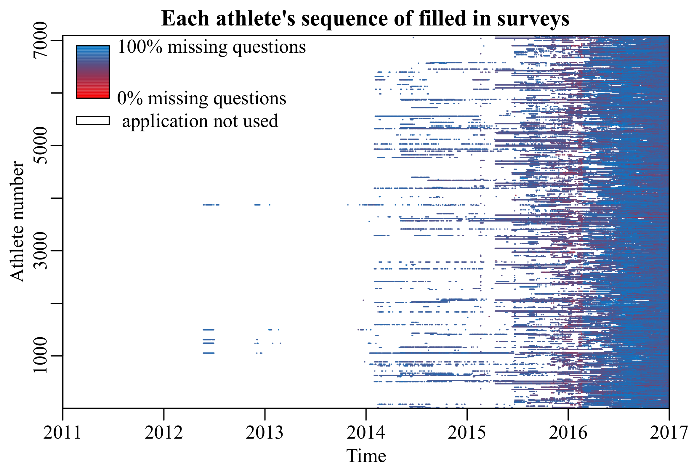
When surveys are included in the models that drive these applications, missing data are a persistent problem due to unanswered questions, or even entire missing surveys (Figure 1) [12,13]. Developers could choose to make each question mandatory to avoid unanswered questions, but this would bias the results towards a group that is inclined to answer every question, or increase the number of entirely missing surveys. Furthermore, the missingness generating process must be taken into account (Table 1). This raises the question of how to deal with missing data in longitudinal surveys.

Figure 1. Survey completion by all athletes. Absence of linepieces indicate ‘missing’ surveys; color indicates the amount of missingness within surveys. There are filled in surveys throughout the entire sequence, although usage in 2011–2012 is so sparse that it appears as though there are none.

Table 1. Description of types of missingness: missing completely at random (MCAR); missing at random (MAR); missing not at random (MNAR) [14].

	MCAR	MAR	MNAR
Meaning	Missingness is not correlated with the outcome.	Missingness could be correlated with other variables.	Missingness is correlated with the outcome.
Example	Question could be overlooked, survey forgotten.	Older individuals could be less inclined to state their weight.	Depressed individuals are less inclined to fill in depression survey.

A common solution to missing data in deep learning is to use indicators for missingness of the original variables [15], such that the model can learn to associate each variables’ missingness with the outcome. However, this still leaves the question of how to impute the missing values in the original data. Moreover, including an indicator for each original variable doubles the input size, which may be problematic for data sets with a low number of observations relative to the number of features. Hence we propose a simple alternative for when the increase in variables is too high given the number of observations by Z-scoring, summing the missingness indicators, including the last recorded outcome in the input, and simplifying the padding of missing surveys.

The golden standard in handling missing data that are MCAR or MAR is through full conditional specification (FCS), which repeatedly imputes missing values of one variable, given the others [16,17]. Each imputation then trains a separate model, and the resulting models are pooled for inference or prediction. By drawing multiple imputations from the posterior, FCS can reflect the variance of the original variables. Furthermore, pre-existing relationships between variables can be preserved through passive imputation, resulting in greater precision [18,19].

A downside to FCS is that it cannot impute data that are MNAR without introducing bias. Moreover, the computational cost is greatly increased by drawing the imputations and separately training models on each of them. Recent literature suggests the required number of imputations depends on the amount of missingness and can even exceed 100, which would increase the computational cost by a hundred-fold from training the individual models alone [20].

Gondara and Wang (2017) [21] proposed training a denoising autoencoder on corrupted copies of a complete subset of the training data, minimizing the reconstruction error on the non-corrupt, non-missing subset. For purely predictive purposes, their method requires considerably less domain knowledge to use correctly compared to FCS, since the model automatically learns relationships between variables, rather than requiring careful consideration of each variable’s imputation method. Moreover, in their experiments, the autoencoder outperformed FCS both in terms of predictive accuracy and computational cost. However, their method relies on two strong assumptions: Firstly, there must be a large enough complete subset of the data to train such an autoencoder and secondly, this complete subset must accurately represent the incomplete data (i.e., missing data are MCAR).

Lipton et al., (2016) [15] proposed simply including indicators for missingness of the original variables (Equation (1)), followed by 0–1 normalization (Equation (4)) and zero imputation. This method has the strong advantage that the model can learn direct relationships between missingness and the response, meaning that it should be able to model even MNAR. However, the number of variables can be increased by up to a two-fold, depending on how many columns contain missing values. For survey data largely consisting of partial entries, the individual missingness vectors may not bear enough information to justify the resulting increase in parameters. That is to say, the response variable might simply correlate with the number of questions an individual is inclined to answer on a given day.

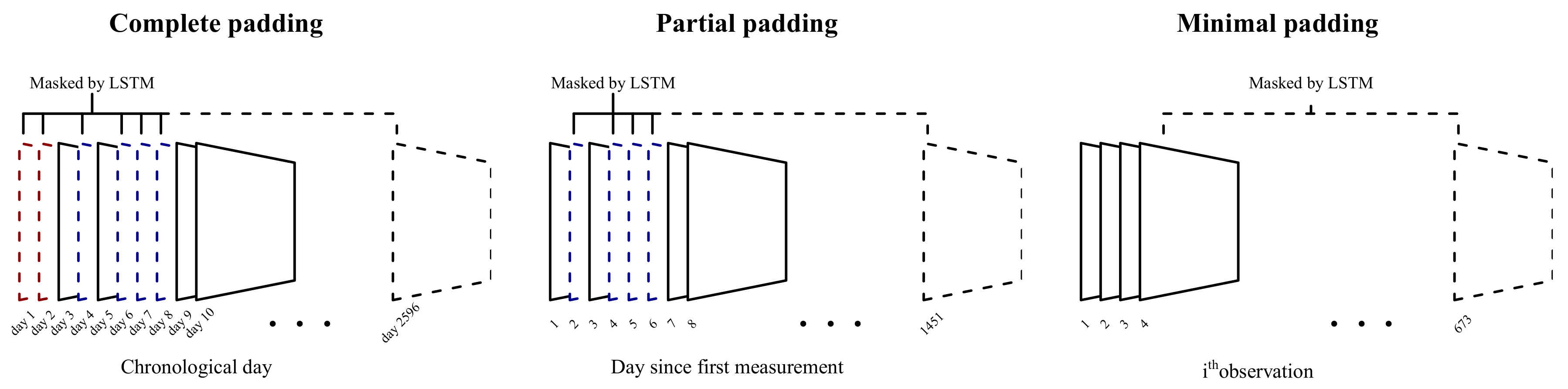
Hence we propose a simple alternative for when the amount of missingness sufficiently correlates with the outcome by summing the missingness indicators (Equation (2)), followed by Z-scoring (Equation (3)) of the non-binary features, including the last recorded outcome in the input, and simplifying the padding of entirely missing surveys (Figure 2).

Figure 2. Example of a sequence of surveys. Dashed surveys are missing (red: prior to first entry; blue: between entries; black: variable sequence length until the participant’s last entry).

2. Materials and Methods

This study has been approved by the ethical committee of Tokyo Institute of Technology under the approval number 2018069.

2.1. Description of Data

Repeated survey data spanning a 7-year period (2011–2017) was collected from a mobile application. This application was made available to 7098 athletes in Japan. Of these athletes, 5970 had at least one recorded outcome. These were randomly distributed into a train (80%), validation (10%), and test set (10%), each containing surveys from different athletes.

The survey consisted of 65 questions regarding the athletes’ physical activity, food intake, and biometric data (e.g., weight, body fat percentage) on a particular day. The outcome variable was the self-assessed condition on that day, ranging from 1 (very poor) to 10 (very good). Since the data are sparse and contain a considerable amount of missing data, the outcome variable was discretized to good condition (≥6) or poor condition (<6) to simplify the prediction problem to binary classification.

In total, $70.1\%$ of survey answers on filled in surveys were missing. Questions which were answered less than $5\%$ of the time were omitted, since these bear little information about the average user of the application. On average, participants only filled in the survey $2.9\%$ of all days, leaving a large number of missing days (Figure 1).

2.2. Imputation

For the FCS approach, $m=5$ imputed data sets were generated, as recommended by Van Buuren (2016) [16]. Although recent literature suggests a larger m might be more precise [20], the computation time already far exceeded other methods, taking upwards of m times as long. Logistic regression was used to impute binary variables and predictive mean matching otherwise.

The missingness indicators approach was implemented in the same manner as described in Lipton et al. (2016) [15], adding a matrix ${\mathbf{X}}^{*}$ of zeroes and ones corresponding to available and missing original data $\mathbf{X}$, respectively as in Equation (1), followed by zero imputation.

$$\begin{array}{c}\hfill \begin{array}{c}\hfill {\mathbf{X}}_{\mathrm{new}}=\left[\mathbf{X},{\mathbf{X}}^{*}\right];x_{ij}^{*}=\left\{\begin{array}{c}1\mathrm{if}{x}_{ij}=\varnothing \hfill \\ 0\mathrm{otherwise}\hfill \end{array}\right.\hspace{1em}\forall x_{ij}\in {\mathbf{X}}_{n\times p}\end{array}\end{array}$$

(1)

where n is the number of observations and p the number of questions on the survey. Categorical variables were restricted to two categories (yes/no), where missingness was imputed by the most sensible alternative. In our method, a missingness variable was added by summing the number of missing values in each row as in Equation (2). Other combinations (mean, standard deviation) were also considered but did not appear to perform better in initial experimentation.

$$\begin{array}{c}\hfill \begin{array}{c}\hfill {\mathbf{X}}_{\mathrm{new}}=\left[\mathbf{X},(1,1,\dots ,1){\mathbf{X}}^{*}\right];x_{ij}^{*}=\left\{\begin{array}{c}1\mathrm{if}{x}_{ij}=\varnothing \hfill \\ 0\mathrm{otherwise}\hfill \end{array}\right.\hspace{1em}\forall x_{ij}\in {\mathbf{X}}_{n\times p}\end{array}\end{array}$$

(2)

Studentized Z-scores were obtained from all non-binary variables using the non-missing training data as follows:

$$\begin{array}{c}\hfill \begin{array}{c}\hfill z_{ij}=\frac{x_{ij}-{\overline{x}}_{·j}}{s_j}\forall x_{ij}\in {\mathbf{X}}_{n\times p}\end{array}\end{array}$$

(3)

where ${\overline{x}}_{·j}$ and $s_j$ are the sample mean and standard deviation of non-missing observations from variable j, respectively. Whereas 0-1 normalization as in Equation (4) followed by zero imputation affects the mean (biased towards zero), Z-scoring as in Equation (3) followed by zero imputation is effectively mean-imputation, preserving the original mean. This assigns a ’neutral’ value to missing values, whereas normalization followed by zero imputation assigns an extreme value. Categorical variables were treated as aforementioned.

$$\begin{array}{c}\hfill \begin{array}{c}\hfill x_{\mathrm{normalized},ij}=\frac{x_{ij}-min\left(x_{·j}\right)}{max\left(x_{·j}\right)-min\left(x_{·j}\right)}\forall x_{ij}\in {\mathbf{X}}_{n\times p}\end{array}\end{array}$$

(4)

2.3. Padding

Most participants filled in the survey sporadically, leaving large gaps in the sequences. Three padding strategies (Figure 2) for these missing days were compared in terms of prediction error. The first involves simply padding all missing days as entries consisting entirely of zeroes (complete padding). These zeroes were then masked in the first layer of the model, allowing the LSTM to ignore these entries. This approach is very similar to that described in Che et al., (2018) [22], except that their version was based on a gated recurrent unit [23]. A quick comparison showed that an LSTM performed better on these data (results not included).

Since participants started using the application at different times, the second method ignores the missing days prior to a participant’s first entry (partial padding). In other words, the first day of entry was considered to be day 1. While this method cannot account for effects of a particular day (e.g., there might have been a national holiday), it reduces the total sequence length, which in turn reduces the model complexity and computational cost.

The third method simply ignores missing days and instead models the available data as an ordered sequence (minimal padding). While this method cannot account for the time between surveys, it further reduces the sequence length.

2.4. Lagged Response

Where available, the last recorded outcome was added to the input. For the first observation, this variable was set to zero instead, treating it in the same way as other missing values. In the results section, this is referred to as LR.

2.5. Experiments

All models consisted of a 3-layer LSTM network with 32, 24 and 16 nodes in the first, second, and third hidden layer, respectively [24]. A combination of non-recurrent and recurrent dropout was used, as proposed by Semeniuta et al. (2016) [25]. Non-recurrent dropout was set to $0.5$ and recurrent dropout to $0.4$. Additional regularization and different layer types were considered, but did not appear to improve accuracy (results not included). Gradient updates were performed in batch sizes equal to the longest complete sequence ($n=673$) using adaptive moment estimation with hyperparameters equal to that of the original paper [26]. Binary crossentropy was minimized on the validation set and overfitting was assessed by discrepancies between training and validation loss. Initial experimentation revealed that validation accuracy plateaued after around 2000 epochs. This number of epochs was used for each comparison in the results section, unless stated otherwise.

All experiments were conducted using the Windows version of the RStudio interface to Keras Tensorflow, with GPU acceleration enabled, on the system summarized in Table 2. ROC statistics were calculated using the ROCR package [27].

Table 2. Hardware used in the experiments.

CPU	i7 7820HK (@3.6 GHz)
GPU	NVidia GTX1070 (8GB VRAM)
RAM	32GB DDR4-2400

3. Results

Model selection was based on (macro) F${}_1$ score on the validation set. The F${}_1$ and area under the receiver operator curve (AUROC) statistics shown in this section were calculated by means of 10-fold cross validation (90% data) and on the independent test set (10% data). See Figure 3 for corresponding ROC curves.

Figure 3. Receiver operator curves corresponding to the AUROC values on the test set in Table 3.

3.1. Imputation

Table 3 shows the performance of FCS, compared to indicators for missingness and a simple count of missingness. Including a lagged response variable (last recorded observation) increased performance of all methods. These results were obtained using the simplest padding strategy (minimal padding).

Table 3. Performance of different imputation strategies. Abbreviations: full conditional specification (FCS), lagged response (LR), indicators (I), missingness count (MC). Our method is the combination MC, LR. The highest test performance is shown in bold.

		10-Fold CV Mean ± Std	Test Performance
F${}_1$	FCS	0.589 ± 0.037	0.585
	FCS, LR	0.591 ± 0.038	0.588
	I	0.679 ± 0.064	0.676
	I, LR	0.701 ± 0.050	0.696
	MC	0.728 ± 0.037	0.723
	MC, LR	0.780 ± 0.039	0.781
AUROC	FCS	0.474 ± 0.106	0.473
	FCS, LR	0.479 ± 0.103	0.477
	I	0.649 ± 0.069	0.645
	I, LR	0.667 ± 0.081	0.648
	MC	0.728 ± 0.079	0.717
	MC, LR	0.751 ± 0.040	0.740

Lipton et al. (2016) [15] normalized their input to $(0,1)$ (Equation (4)), while our method involved standardization (Equation (3)). Hence, a quick comparison is included using either scaling technique in conjunction with our method, which shows standardization resulted in better performance than normalization on these data (Table 4).

Table 4. Comparison of scaling methods, using a lagged response variable and a missingness count. The highest test performance is shown in bold.

		10-Fold CV Mean ± Std	Test Performance
F${}_1$	Unscaled	0.623 ± 0.078	0.618
	Standardized	0.780 ± 0.039	0.781
	Normalized	0.578 ± 0.064	0.576
AUROC	Unscaled	0.613 ± 0.084	0.601
	Standardized	0.751 ± 0.040	0.740
	Normalized	0.474 ± 0.061	0.465

3.2. Padding

Compared to the simplest strategy (minimal padding), padding the missing days in between measurements (partial padding) more than doubled the median training time per epoch (Table 5), while underperforming the unpadded approach (Table 6). Padding the missing days chronologically (complete padding) took even longer and resulted in inability to determine the test error, presumably due to the resulting large gaps in between observations and poor overlap between different individuals’ dates of filling in the survey.

Table 5. Seconds per epoch for different padding strategies. The highest performance is shown in bold.

	Minimal	Partial	Complete
Time per epoch (s)	35	81	145

Table 6. Comparison of padding strategies after 2k, 4k, and 6k epochs. The highest test performance is shown in bold.

		10-Fold CV Mean ± Std	Test Performance
F${}_1$	Minimal (2k)	0.780 ± 0.039	0.781
	Minimal (4k)	0.796 ± 0.034	0.795
	Minimal (6k)	0.796 ± 0.034	0.796
	Partial (2k)	0.779 ± 0.037	0.776
	Partial (4k)	0.787 ± 0.036	0.785
	Partial (6k)	0.788 ± 0.038	0.788
	Complete (2k)	-	-
	Complete (4k)	-	-
	Complete (6k)	-	-
AUROC	Minimal (2k)	0.751 ± 0.040	0.740
	Minimal (4k)	0.754 ± 0.044	0.743
	Minimal (6k)	0.758 ± 0.045	0.750
	Partial (2k)	0.723 ± 0.062	0.719
	Partial (4k)	0.736 ± 0.051	0.731
	Partial (6k)	0.735 ± 0.047	0.731
	Complete (2k)	-	-
	Complete (4k)	-	-
	Complete (6k)	-	-

To assess whether the padded approaches simply plateaued later than the minimal approach, testing accuracy was also assessed beyond the heuristically defined plateau at 2000 epochs. While a slight increase in accuracy after the additional training time was indeed observed, the minimal padding approach equally benefitted from the additional epochs.

4. Discussion

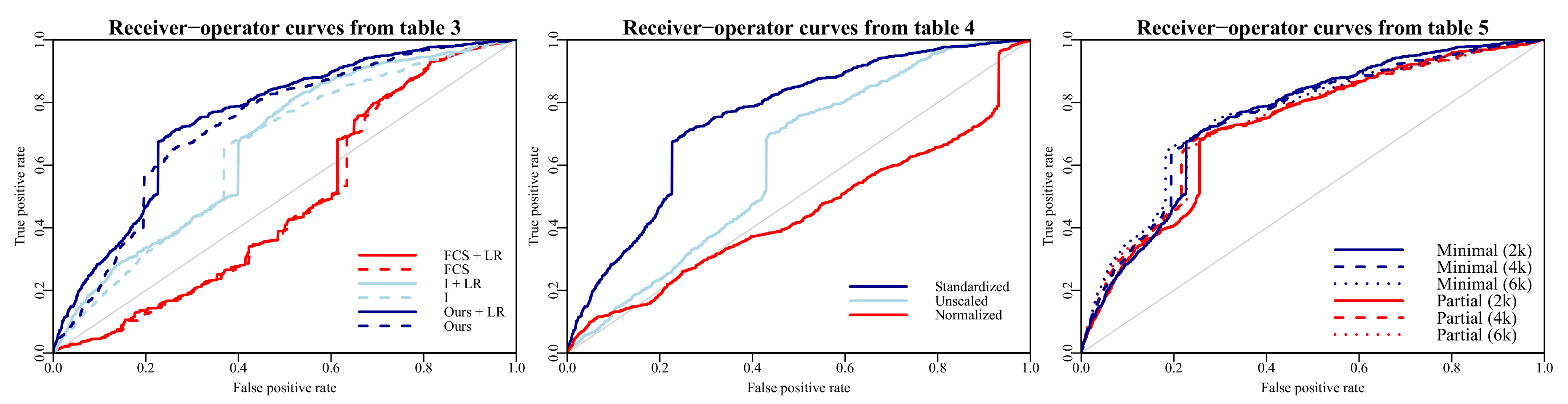
The FCS approach with $m=5$ imputations underperformed all other methods, both in terms of prediction accuracy and computation time (increased by a factor m). The most likely explanation for its subpar accuracy is that the missing data were MNAR, and FCS is not suitable for MNAR. This assertion is supported by the increased performance observed when directly specifying missingness through indicators (Table 3). Another contributing factor might be that the amount of missingness ($70.1\%$ on filled in surveys; $98.9\%$ in total) is simply too large, causing issues when imputing missing data and then ‘reusing’ the data for the predictive model.

While FCS might have benefitted from a considerably larger number of imputations, it was already the most computationally costly method. Since model averaging generally tends to increase performance, the additional computation time—if available—might perhaps be better spent on e.g., bagging other methods, rather than drawing additional imputations with FCS.

Interestingly, correctly padding and masking the missing days did not improve accuracy, nor did the forward filling strategy proposed in Lipton et al. (2016) [15]. The former could either be attributed to a small effect of time in between survey entries on the outcome, or inability of the model to learn this effect using the number of observations at hand ($n_{\mathrm{train}}=4776$) in conjunction with the high amount of missingness. A limitation of this comparison is that we did not further investigate how different regularization techniques might have affected the performance of the padding strategies. The forward filling strategy might be better justifiable for clinical data, where measurements are taken at intervals after which they are expected to change.

While ignoring the missing days resulted in the greatest performance (Table 6), reasonable performance could also be achieved by masking and padding the missing days in between measurements. This method might achieve higher accuracy on problems where the time in between observations is of greater relevance to the outcome.

These results demonstrate that with appropriate adjustments, a deep learning algorithm can even learn reasonably from a sparse sequence of gappy data. Various simplifications of previously suggested methods greatly reduced computational time, while simultaneously outperforming more costly methods in terms of prediction accuracy. The greatest accuracy was achieved on these data, by including a LR variable and a count of the missing variables, followed by Z-scoring and zero imputation.

Importantly, our method does not require a subset of the data which is complete, nor does it require the missing data to be MCAR or MAR. It must be noted, however, that our method might not perform well if the amount of missingness is not as informative about the outcome as it is in these survey data. Future work can demonstrate whether this approach also performs well on other time series with various forms of missingness.