Frequency Response Analysis of Perforated Shells with Uncertain Materials and Damage

Abstract

In this paper, we give an overview of the issues one must consider when designing methods for vibration based health monitoring systems for perforated thin shells especially in relation to frequency response analysis. In particular, we allow either the material parameters or the structure or both to be random. The numerical experiments are computed using the standard high order finite element method with stochastic collocation for the cases with random material and Monte Carlo for those with damaged or random structures. The results display a wide range of responses over the experimental configurations. In perforated shell structures, the internal boundary layers can play an important role especially when damage is allowed within the penetration patterns. The computational methodology advocated here can be used to build statistical databases that are necessary for development of probabilistic damage identification methods.

1. Introduction

Vibration based structural health monitoring remains a vibrant research area with an extensive body of literature. A review article from 2004 by Carden and others [1] alone cites over 150 publications. A more recent (2011) review article is by Fan and Qiao [2] concentrating on damage identification methods. To use the language of inverse problems, modelling of damage identification methods requires the forward part, i.e., simulation of the mechanical systems we are interested in, and the inverse part or identification of the structure or changes within. In this paper, we give an overview of the issues one must consider when designing methods for vibration based health monitoring systems for perforated thin shells, especially in relation to frequency response analysis.

Engineering constructions made of perforated materials are challenging from the computational mechanics point of view. Some examples of relevant industrial constructions are drying drums and Trommel screens. However, the literature on perforated materials is somewhat sparse. The introduction in Martikka et al. [3] serves as an excellent overview of the complexities of perforated shell designs—our interest—and their applications.

It is natural to seek a simplified problem via homogenization, a process where the material properties of a non-perforated structure are adjusted to match those of the perforated one. Recently, Jhung and his collaborators have published a number of papers within the nuclear reactor design context, see [4,5,6]. For a detailed and exhaustive case study for a single cylindrical shell submerged in fluid, see [7]. In this paper, however, we do not advocate such an approach. The homogenization of shell structures under loading and especially in dynamic settings is not well understood. The main culprit is that this class of engineering problems is a parameter-dependent problem, where the parameter is the (dimensionless) thickness. It is characteristic of such problems that there are local features in the solution that vary in size and amplitude depending on the parameter and one can always define a critical value of the parameter where the local features become dominant, and homogenization fails. In frequency response analysis, there is an added complication. Let us consider shells of revolution. It follows immediately that in free vibration the eigenmodes must have integer valued wave numbers in the angular part of the mode. This wave number in turn depends on the parameters of the problem, including the shell geometry and the material parameters; see [8]. Thus, successful homogenization would require matching of modes which would be a more difficult problem than simply associating the first ten modes, say, in both cases. In addition, the dependence on the shell geometry means that it is not feasible to homogenize a perforated plate (a sheet of metal) and then ignore the effects of the curvature changes.

Here, we are interested in the frequency response of perforated shells when either the material parameters such as Young’s modulus or the structure or both are random in a well-defined way. The structural randomness is introduced via a simple damage model where the perforation patterns are perturbed with uniform intensity over the whole domain. We study two structures, a cylindrical shell which is of practical importance, and an example of different shell geometry, a perforated hyperbolic shell (cooling tower), which is more of an academic interest but serves to underline the central issues. It follows naturally that inclusion of uncertainty in the simulations leads to distribution of frequency responses that require statistical analysis [9].

The main contribution of this work can be divided into two interconnected parts: First, through understanding and analysis of the model problems, we can design a set of experiments that illustrate the expected phenomena, and, second, the experiments can be computed and the results analyzed within the standard stochastic framework. We see that in multi-parametric problems the responses can be widely varying as well. In perforated shell structures, the internal boundary layers can play an important role, especially when damage is allowed within the penetration patterns. The computational methodology advocated here can be used to build statistical databases that are necessary for development of probabilistic damage identification methods. The important observation is that at least in some cases the distributions of quantities of interest in such settings can be recovered and hopefully utilized in the design of, e.g., damage identification methods.

All simulations are computed with an $hp$-version of the finite element method [10,11], using standard elements. This choice is based on our desire to avoid any issues related to numerical locking.

The rest of the paper is structured as follows: In Section 2, we discuss the deterministic shell eigenproblems and issues specific to perforated structures; Section 3 sets the reference results for the free vibration of our model structures. The important concept of mixing of modes is demonstrated by comparing results over perforated and non-perforated shell geometries; frequency response analysis under uncertainty is briefly outlined in Section 4; our extensive set of numerical experiments is the topic of Section 5; Finally, conclusions are drawn in Section 6.

2. Preliminaries

In this section, the basic characteristics of perforated shell problems are introduced. Much of the material has been covered in the literature before, but here the notations have been normalized to conform to discussion in this paper. We assume that the reader is familiar with the finite element method and do not cover it here at all. It is also assumed that the existence of internal boundary layers in structures is at least accepted.

The shell problem is discussed as an eigenproblem, since it is the underlying problem despite the eventual formulation of the actual frequency response problem below. The dimensionally reduced shell model and the effect of the shell geometry are outlined in this context.

Special issues related to perforated domains are the penetration patterns, here with the damage model, and in the shell context the boundary layers. All three are briefly covered in this section as well.

2.1. Shell Eigenproblems

Assuming a time harmonic displacement field, the free vibration problem for a general shell leads to the following abstract eigenvalue problem: Find $\mathbf{u}\in {\mathbb{R}}^3$ and ${\omega }^2\in \mathbb{R}$ such that

$$\left\{\begin{array}{c}\mathbf{S}\mathbf{u}={\omega }^2\mathbf{M}\mathbf{u}\hfill \\ +\mathrm{boundary} \mathrm{conditions}.\hfill \end{array}\right.$$

(1)

Above, $\mathbf{u}=\{u,v,w\}$ represents the shell displacement field, while ${\omega }^2$ represents the square of the eigenfrequency. In the abstract setting, $\mathbf{S}$ and $\mathbf{M}$ are differential operators representing deformation energy and inertia, respectively. In the discrete setting, they refer to corresponding stiffness and mass matrices.

2.1.1. Shell Geometry

In the following, we denote $\mathbf{x}=(x_1,x_2,x_3)\in {\mathbb{R}}^3$ and let a profile function $x_2=f\left(x_1\right)$ revolve about the $x_1$-axis. Naturally, the profile function defines the local radius of the shell. Shells of revolution can now formally be characterized as domains in ${\mathbb{R}}^3$ of type

$$\mathsf{\Omega }=\left\{\mathbf{x}+\eta \left(\mathbf{x}\right)\mathbf{n}\left(\mathbf{x}\right)|\mathbf{x}\in \widehat{D},-d_0\left(\mathbf{x}\right)<\eta \left(\mathbf{x}\right)<d_1\left(\mathbf{x}\right)\right\},$$

(2)

where $\widehat{D}$ is a (mid)surface of revolution, $\mathbf{n}\left(\mathbf{x}\right)$ is the unit normal to $\widehat{D}$, and $d\left(\mathbf{x}\right)=d_1\left(\mathbf{x}\right)+d_0\left(\mathbf{x}\right)$ is the thickness of the shell measured in the direction of the normal. An illustration of such configurations is given in Figure 1. Throughout this paper, we consider parabolic and hyperbolic shells with profile functions $f_P\left(x_1\right)=1$ and $f_H\left(x_1\right)=1+{(x_1/\pi )}^2$, respectively. This classification of surfaces follows from Gaussian theory of surfaces, where it holds that for general profile functions $f^{″}\left(x_1\right)=0$ for parabolic, and $f^{″}\left(x_1\right)>0$ for hyperbolic surfaces.

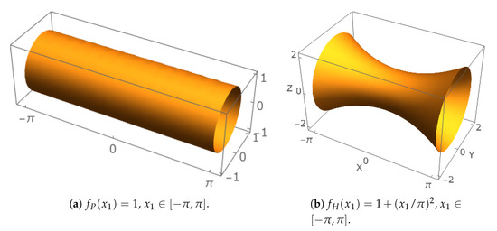
Figure 1. Shell geometries. Parabolic and hyperbolic examples with profile functions $f_P\left(x_1\right)=1$ and $f_H\left(x_1\right)=1+{(x_1/\pi )}^2$, respectively. Notice the scaling of the subfigures, in both cases $x_1\in [-\pi ,\pi ]$. The shells of revolution are shown in ${\mathbb{R}}^3$, with $x_1$- and x-coordinates coinciding.

Let us have $d\left(\mathbf{x}\right)=d$ (constant) and define principal curvature coordinates, where only four parameters, the radii of principal curvature $R_1$, $R_2$, and the so-called Lamé parameters, $A_1$, $A_2$, which relate coordinates changes to arc lengths, are needed to specify the curvature and the metric on $\widehat{D}$. The displacement vector field of the midsurface $\mathbf{u}=\{u,v,w\}$ can be interpreted as projections to directions  

$${\mathbf{e}}_1=\frac{1}{A_1}\frac{\partial \mathsf{\Psi }}{\partial x_1},{\mathbf{e}}_2=\frac{1}{A_2}\frac{\partial \mathsf{\Psi }}{\partial x_2},{\mathbf{e}}_3={\mathbf{e}}_1\times {\mathbf{e}}_2,$$

(3)

where $\mathsf{\Psi }(x_1,x_2)$ is a suitable parametrization of the surface of revolution, ${\mathbf{e}}_1,{\mathbf{e}}_2$ are the unit tangent vectors along the principal curvature lines, and ${\mathbf{e}}_3$ is the unit normal. In other words,

$$\mathbf{u}=u{\mathbf{e}}_1+v{\mathbf{e}}_2+w{\mathbf{e}}_3.$$

(4)

Assuming that the shell profile is given by $f\left(x_1\right)$, the geometry parameters are

$$A_1\left(x_1\right)=\sqrt{1+{\left[f^{\prime }\left(x_1\right)\right]}^2},A_2\left(x_1\right)=f\left(x_1\right),$$

(5)

and

$$R_1\left(x_1\right)=-\frac{A_1{\left(x_1\right)}^3}{f^{″}\left(x_1\right)}, R_2\left(x_1\right)=A_1\left(x_1\right)A_2\left(x_1\right).$$

(6)

We can now define the dimensionless thickness t as $t=d/R$, where $R\sim R_2$ is the unit length. In the following we assume that $R\sim 1$ and thus use the two thickness concepts denoted by d and t interchangeably.

2.1.2. Reduction in Thickness

The free vibration problem for a general shell (1) in the case of shell of revolution with constant thickness t leads to the following eigenvalue problem: Find $\mathbf{u}\left(t\right)$ and ${\omega }^2\left(t\right)\in \mathbb{R}$ such that

$$\left\{\begin{array}{c}t{A}_m\mathbf{u}\left(t\right)+t{A}_s\mathbf{u}\left(t\right)+t^3{A}_b\mathbf{u}\left(t\right)={\omega }^2\left(t\right)M\left(t\right)\mathbf{u}\left(t\right)\hfill \\ +\mathrm{boundary\; conditions}.\hfill \end{array}\right.$$

(7)

Again, $\mathbf{u}\left(t\right)$ represents the shell displacement field, while ${\omega }^2\left(t\right)$ represents the square of the eigenfrequency. The differential operators $A_m$, $A_s$, and $A_b$ account for membrane, shear, and bending potential energies, respectively, and are independent of t. Finally, $M\left(t\right)$ is the inertia operator, which in this case can be split into the sum $M\left(t\right)=t{M}^l+t^3{M}^r$, with $M^l$ (displacements) and $M^r$ (rotations) independent of t.

Let us next consider the variational formulation of problem (7). Accordingly, we introduce the space V of admissible displacements, and consider the problem: Find $(\mathbf{u}\left(t\right),{\omega }^2\left(t\right))\in V\times \mathbb{R}$ such that

$$\begin{array}{c}\hfill t{a}_m(\mathbf{u}\left(t\right),\mathbf{v})+t{a}_s(\mathbf{u}\left(t\right),\mathbf{v})+t^3{a}_b(\mathbf{u}\left(t\right),\mathbf{v})=\\ \hfill {\omega }^2\left(t\right)m(t;\mathbf{u}\left(t\right),\mathbf{v})\forall \mathbf{v}\in V,\end{array}$$

(8)

where $a_m(·,·)$, $a_s(·,·)$, $a_b(·,·)$ and $m(t;·,·)$ are the bilinear forms associated with the operators $A_m$, $A_s$, $A_b$ and $M\left(t\right)$, respectively. Obviously, the space V and the three bilinear forms depend on the chosen shell model (see for instance [12]).

2.1.3. Two-Dimensional Model

Our two-dimensional shell model is the so-called Reissner–Naghdi model [12], where the transverse deflections are approximated with low-order polynomials. The resulting vector field has five components $\mathbf{u}=(u,v,w,\theta ,\psi )$, where the first three are the standard displacements and the latter two are the rotations in the axial and angular directions, respectively. Here, we adopt the convention that the computational domain $D\subset {\mathbb{R}}^2$ is given by the surface parametrisation and the axial/angular coordinates are denoted by x and y:

$$D=\left\{\right(x,y\left)\right|a\le x\le b,0\le y<2\pi \}.$$

(9)

Deformation energy $\mathcal{A}(\mathbf{u},\mathbf{u})$ is divided into bending, membrane, and shear energies, denoted by subscripts B, M, and S, respectively:

$$\mathcal{A}(\mathbf{u},\mathbf{u})=t^2{\mathcal{A}}_B(\mathbf{u},\mathbf{u})+{\mathcal{A}}_M(\mathbf{u},\mathbf{u})+{\mathcal{A}}_S(\mathbf{u},\mathbf{u}).$$

(10)

Notice that we can safely cancel out one power of t.

Bending, membrane, and shear energies are given as [13]

$$\begin{array}{c}\hfill t^2{\mathcal{A}}_B(\mathbf{u},\mathbf{u})=t^2{\int }_{{\widehat{\mathsf{\Omega }}}_t}E(x,y)[\nu {({\kappa }_{11}\left(\mathbf{u}\right)+{\kappa }_{22}\left(\mathbf{u}\right))}^2\\ \hfill +(1-\nu )\sum _{i,j=1}^2{\kappa }_{ij}{\left(\mathbf{u}\right)}^2]A_1(x,y)A_2(x,y)dxdy,\end{array}$$

(11)

$$\begin{array}{c}\hfill {\mathcal{A}}_M(\mathbf{u},\mathbf{u})=12{\int }_{{\widehat{\mathsf{\Omega }}}_t}E(x,y)[\nu {({\beta }_{11}\left(\mathbf{u}\right)+{\beta }_{22}\left(\mathbf{u}\right))}^2\\ \hfill +(1-\nu )\sum _{i,j=1}^2{\beta }_{ij}{\left(\mathbf{u}\right)}^2]A_1(x,y)A_2(x,y)dxdy,\end{array}$$

(12)

$$\begin{array}{c}\hfill {\mathcal{A}}_S(\mathbf{u},\mathbf{u})=6(1-\nu ){\int }_{{\widehat{\mathsf{\Omega }}}_t}E(x,y)\left[({\rho }_1{\left(\mathbf{u}\right)}^2+{\rho }_2{\left(\mathbf{u}\right)}^2)\right]\times \\ \hfill A_1(x,y)A_2(x,y)dxdy,\end{array}$$

(13)

where $\nu$ is the Poisson ratio (constant), and $E(x,y)$ is the Young’s modulus with scaling $1/\left(12(1-{\nu }^2)\right)$.

The symmetric 2D strains, bending ($\kappa$), membrane ($\beta$), and shear ($\rho$), are defined as

$$\begin{array}{cc}\hfill {\kappa }_{11}& =\frac{1}{A_1}\frac{\partial \theta }{\partial x}+\frac{\psi }{A_1{A}_2}\frac{\partial A_2}{\partial y},\hfill \end{array}$$

(14)

$$\begin{array}{cc}\hfill {\kappa }_{22}& =\frac{1}{A_2}\frac{\partial \psi }{\partial y}+\frac{\theta }{A_1{A}_2}\frac{\partial A_2}{\partial x},\hfill \end{array}$$

(15)

$$\begin{array}{cc}\hfill {\kappa }_{12}& =\frac{1}{2}\left[\frac{1}{A_1}\frac{\partial \psi }{\partial x}+\frac{1}{A_2}\frac{\partial \theta }{\partial y}\right.\hfill \\ \hfill & -\frac{\theta }{A_1{A}_2}\frac{\partial A_2}{\partial y}-\frac{\psi }{A_1{A}_2}\frac{\partial A_2}{\partial x}\hfill \\ \hfill & -\frac{1}{R_1}\left(\frac{1}{A_2}\frac{\partial u}{\partial y}-\frac{v}{A_1{A}_2}\frac{\partial A_2}{\partial x}\right)\hfill \\ \hfill & -\left.\frac{1}{R_2}\left(\frac{1}{A_1}\frac{\partial v}{\partial x}-\frac{u}{A_1{A}_2}\frac{\partial A_1}{\partial y}\right)\right],\hfill \end{array}$$

(16)

$$\begin{array}{cc}\hfill {\beta }_{11}& =\frac{1}{A_1}\frac{\partial u}{\partial x}+\frac{v}{A_1{A}_2}\frac{\partial A_1}{\partial y}+\frac{w}{R_1},\hfill \end{array}$$

(17)

$$\begin{array}{cc}\hfill {\beta }_{22}& =\frac{1}{A_2}\frac{\partial v}{\partial y}+\frac{u}{A_1{A}_2}\frac{\partial A_2}{\partial x}+\frac{w}{R_2},\hfill \end{array}$$

(18)

$$\begin{array}{cc}\hfill {\beta }_{12}& =\frac{1}{2}\left(\frac{1}{A_1}\frac{\partial v}{\partial x}+\frac{1}{A_2}\frac{\partial u}{\partial y}\right.\hfill \\ \hfill & -\left.\frac{u}{A_1{A}_2}\frac{\partial A_1}{\partial y}-\frac{v}{A_1{A}_2}\frac{\partial A_2}{\partial x}\right),\hfill \end{array}$$

(19)

$$\begin{array}{cc}\hfill {\rho }_1& =\frac{1}{A_1}\frac{\partial w}{\partial x}-\frac{u}{R_1}-\theta ,\hfill \end{array}$$

(20)

$$\begin{array}{cc}\hfill {\rho }_2& =\frac{1}{A_2}\frac{\partial w}{\partial y}-\frac{v}{R_2}-\psi .\hfill \end{array}$$

(21)

In our experiments, the shell profiles are functions of x only, but not necessarily constant, hence the strains are presented in a general form.

The stiffness matrix $\mathbf{S}$ is obtained after integration and assembly. Here, the mass matrix $\mathbf{M}$ is the standard 2D one with density $\sigma$ except for the scaling of the rotation components and surface differential $A_1(x,y)A_2(x,y)$.

2.2. Perforated Domains

Perforated domains are characterized by the penetration patterns which in turn depend on the underlying manufacturing processes and the related hole coverage, typically given as a percentage. Here, we consider standard structured patterns and extend the concepts to quasi-random patterns. We also consider a simple randomized damage model.

2.2.1. Penetration Patterns

The quantity used to characterize perforated sheets of metal is the ligament efficiency $\eta$. Let us assume that the holes are ellipses with a, b as the horizontal and perpendicular semi-axis, and the separation of the centres is $P_x$ and $P_y$, respectively. Following [5,14,15], we define horizontal and perpendicular ligament efficiency, denoting them ${\eta }_x$, ${\eta }_y$, respectively. For regular arrays of holes

$${\eta }_x=(P_x-2a)/P_x,{\eta }_y=(P_y-2b)/P_y,$$

(22)

and for triangular arrays, allowing for alternating layers,

$${\eta }_x=(P_x-4a)/P_x,{\eta }_y=(P_y-4b)/P_y.$$

(23)

For circular holes, the radius $r=a=b$, of course, and further if the pattern is regular $\eta ={\eta }_x={\eta }_y$. Both pattern types are illustrated in Figure 2. Notice that the triangular pattern in the figure has a tighter packing than that implied by Equation (23).

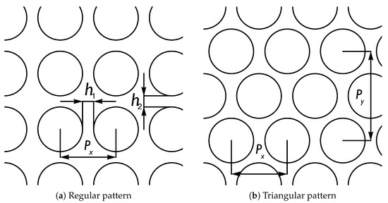
Figure 2. Penetration patterns.

An intriguing option is to replace a regular pattern with one induced by a quasi-random process. Notice that quasi-random means that the process is deterministic which has implications to manufacturing. One of the simplest sequences of points generated by such a process is the Halton sequence [16].

Definition 1 (Halton).

Let $i\in {\mathbb{N}}_0$ and basis $b\in \mathbb{N}$ be such that $b\ge 2$. Then, the inverse representation function ${\varphi }_b\left(i\right)$ is given by

$$i=\sum _{k=1}^{\infty }{i}_k{b}^{k-1},i_k\in \{0,1,\dots ,b-1\}⟶{\varphi }_b\left(i\right)=\sum _{k=1}^{\infty }\frac{i_k}{b^k}.$$

Let $q_1,q_2,\dots ,q_s$ be the s first primes. The s-dimensional Halton sequence is

$$H(q_1,q_2,\dots ,q_s)={\{{\varphi }_{q_1}\left(i\right),{\varphi }_{q_2}\left(i\right),\dots ,{\varphi }_{q_s}\left(i\right)\}}_{i=0}^{\infty }.$$

The choice of the primes is crucial, and, in the context of this paper, only two have to be chosen. The effect of this selection is shown in Figure 3, where the local structures of two sequences are compared. As can be seen from the definition of the Halton sequences, in 2D, the points populate the unit square ${[0,1]}^2$ and have to be mapped to the actual computational domain. We do not attempt to define averaging ligament efficiencies for such penetration patterns.

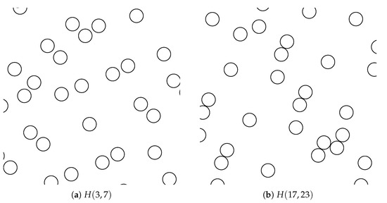
Figure 3. Quasi-random penetration patterns of Halton type. Samples are taken from a 1600 point set at $[-2/5,2/5]\times [\pi -2/5,\pi +2/5]$. The sequences have been selected by trial and error.

However, a useful concept used to relate different kinds of patterns is the cell size $ϵ$, which is the size of the cell containing exactly one hole on average. In the case of a regular $n\times n$-grid on a shell of revolution over $(x,y)\in [-\pi ,\pi ]\times [0,2\pi ]$, we have $ϵ=2\pi /n$. In the limit as $ϵ\to 0$, we expect regular and quasi-regular penetration patterns to converge.

2.2.2. Damage Model

Since we are committed to simulating the systems with faithful geometry description, we can similarly adopt a destructive damage model, where cracks between two holes are modelled simply by removing the area between the respective holes. This is illustrated in Figure 4. The model is straightforward: first, a sample X is chosen with intensity $\mu$ from the set of holes C. Every hole $x_i\in X$ is paired with one of its four nearest neighbors, and together they form a damaged region $d_k$. As can be seen in Figure 4b,d, it can happen that, for both holes in a pair $d_k=(x_i,x_j)$, it holds that $x_i\in X$ and $x_j\in X$, $i\ne j$, and thus the damage can spread over a larger region. Thus, one must ensure that the domain remains simply connected.

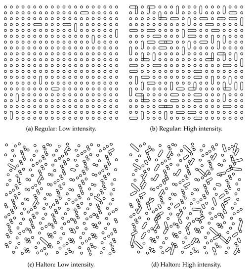
Figure 4. Damage Model. For both regular and quasi-random penetration patterns, damage has been added with uniform global intensity. The regular grid is a $20\times 20$, and the Halton one is $H(5,23)$ with 400 points. Low intensity level for damaged holes is 10/400 and high 100/400.

2.2.3. Layer Chart over Representative Cells

Even though the shell problems are elliptic partial differential equations, the solutions may exhibit local features, formally boundary layers, with characteristic length scales much larger than the chosen cell size $ϵ$. Therefore, it is necessary to review the possible boundary layers that may occur in different scenarios.

For our discussion, it is useful to define the concept of boundary layer generators first (see [17]). The layer generators are independent of the length scale of the problem under consideration.

Definition 2 (Layer Generator).

The subset of the domain from which the boundary layer decays exponentially, is called the layer generator. Formally, the layer generator is of measure zero.

In perforated structures, the hole boundaries are natural layer generators. The boundary layers are not concentrated only around the holes but can emanate along the characteristics of the shell surface. Elliptic, parabolic, and hyperbolic structures each possess a distinctive set of layer deformations. The layer structure is classically assumed to be an exponential solution to the homogeneous Euler equations of the shell problem. In Pitkäranta, Matache, and Schwab [17], it is shown using the Ansatz

$$\mathbf{u}(s,r)=\mathbf{U}{e}^{\lambda s}{e}^{\mathrm{i}kr}$$

(24)

that solutions with $\mathrm{Re}\lambda <0$ such that the characteristic lengths $L=1/\mathrm{Re}\lambda \to 0$ are of the form $L\sim d^{1/n}$, where $n\in \{1,2,3,4\}$. Here, s is the coordinate orthogonal to the layer generator and r the one along it. From these, the layer with $n=2$ is present in all geometries, whereas layers with $n=3$ and $n=4$ are present only in hyperbolic and parabolic geometries, respectively, and thus play a role here as well. The case $n=1$, i.e., the shortest one arises from a shear deformation and can be captured by the shallow shell formulation [17], if necessary. In the 3D visualizations for the very thin case (Figure 5b and Figure 6b), distinct features of the solution, that is, the boundary layers, are clearly visible. In Figure 7, the layer chart is given both for the parabolic and hyperbolic representative cells, with the exception of the shortest one, which is present on every boundary.

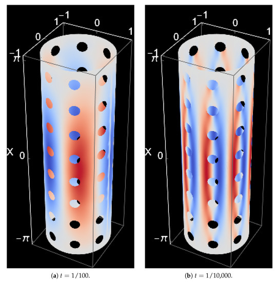
Figure 5. Parabolic shell. Regular $8\times 8$ pattern. The smaller thickness is chosen to conform with a natural characteristic length scale $\sqrt[4]{t}$.

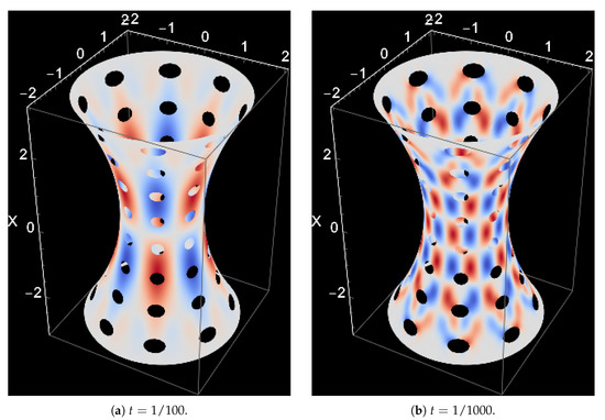
Figure 6. Hyperbolic shell. Regular $8\times 8$ pattern. The smaller thickness is chosen to conform with a natural characteristic length scale $\sqrt[3]{t}$.

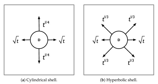
Figure 7. Representative cells: Layer charts with one hole D. The characteristic length scales are indicated in terms of the dimensionless thickness. In the hyperbolic case for the non-axial layers, the directions depend on the actual geometry, in this case, the decay is in the orthogonal direction to the one indicated by the arrow.

3. Free Vibration of Reference Configurations

In this section, we establish the reference configurations on which the numerical experiments below are based and explain the rationale for these experiments. As already given above, the profile functions are $f_P\left(x_1\right)=1$ and $f_H\left(x_1\right)=1+{(x_1/\pi )}^2$, for the parabolic and hyperbolic cases, respectively.

In Table 1, the first 10 eigenpairs are tabulated for both non-perforated shells with $t=1/100$. In the two other tables (Table 2 and Table 3), the first 10 eigenpairs are listed for perforated configurations, including quasi-random ones. The eigenmodes are characterized using axial ($K_x$) and angular ($K_y$) wave numbers, where the fractional axial wave numbers refer to symmetric modes that is, the pair $(K_x,K_y)=(1/2,4)$ refers to mode $\phi (x,y)\sim cos(x/2)cos\left(4y\right)$ or $\phi (x,y)\sim cos(x/2)sin\left(4y\right)$ due to symmetry. The numbers are universal, that is, no material parameters are included except for the Poisson ratio $\nu =1/3$. For non-perforated shells, every eigenvalue (disregarding torsional modes) is a double one due to symmetry. Theoretically, the lowest mode can have an order four, but this occurs only at critical values of t which is not the case here. Even for perforated shells, the eigenvalues are observed to appear in clusters of two.

Table 1. Reference results for the non-perforated test cases. Parameters: $p=8$, $t=1/100$; No material scaling.

a Parabolic				b Hyperbolic
$\mathit{k}$	$\mathit{\lambda }$	${\mathit{K}}_{\mathit{x}}$	${\mathit{K}}_{\mathit{y}}$	$\mathit{k}$	$\mathit{\lambda }$	${\mathit{K}}_{\mathit{x}}$	${\mathit{K}}_{\mathit{y}}$
1	0.0325658	1/2	4	1	0.129749	3/2	5
2	0.0325658	1/2	4	2	0.129749	3/2	5
3	0.0344515	1/2	3	3	0.136477	2	5
4	0.0344515	1/2	3	4	0.136477	2	5
5	0.0613855	1/2	5	5	0.138588	2	4
6	0.0613855	1/2	5	6	0.138588	2	4
7	0.0920303	1	4	7	0.142168	3/2	4
8	0.0920303	1	4	8	0.142168	3/2	4
9	0.0922696	1	5	9	0.156955	2	6
10	0.0922696	1	5	10	0.156955	2	6

Table 2. Parabolic. Parameters: $ϵ=2\pi /20$, $t=1/100$; No material scaling.

a Regular				b Halton: $\mathit{H}(7,37)$
$\mathit{k}$	$\mathit{\lambda }$	${\mathit{K}}_{\mathit{x}}$	${\mathit{K}}_{\mathit{y}}$	$\mathit{k}$	$\mathit{\lambda }$	${\mathit{K}}_{\mathit{x}}$	${\mathit{K}}_{\mathit{y}}$
1	0.028346	1/2	4	1	0.0275997	1/2	3
2	0.0283483	1/2	4	2	0.0280266	1/2	3
3	0.0288704	1/2	3	3	0.0282583	1/2	4
4	0.028872	1/2	3	4	0.0286645	1/2	4
5	0.0543918	1/2	5	5	0.0551038	1/2	5
6	0.0543927	1/2	5	6	0.0553621	1/2	5
7	0.0773403	1	4	7	0.0743065	1/2	2
8	0.0773436	1	4	8	0.0744545	1/2	2
9	0.0779846	1/2	2	9	0.075735	1	4
10	0.0779899	1/2	2	10	0.0759866	1	4

Table 3. Hyperbolic. Parameters: $ϵ=2\pi /30$, $t=1/100$; No material scaling.

a Regular				b Halton: $\mathit{H}(7,37)$
$\mathit{k}$	$\mathit{\lambda }$	${\mathit{K}}_{\mathit{x}}$	${\mathit{K}}_{\mathit{y}}$	$\mathit{k}$	$\mathit{\lambda }$	${\mathit{K}}_{\mathit{x}}$	${\mathit{K}}_{\mathit{y}}$
1	0.108012	3/2	5	1	0.106164	3/2	5
2	0.108026	3/2	5	2	0.106785	3/2	5
3	0.112789	2	5	3	0.110631	1	4
4	0.112798	2	5	4	0.110981	1	4
5	0.112905	1	4	5	0.113495	2	5
6	0.112909	1	4	6	0.113902	2	5
7	0.114934	3/2	4	7	0.114367	3/2	4
8	0.114939	3/2	4	8	0.114711	3/2	4
9	0.132725	2	6	9	0.131692	2	6
10	0.132736	2	6	10	0.132256	2	6

The discrepancies between the eigenvalues in a cluster are a simple measure of homogeneity. In the Halton cases, the discrepancies are larger than in the regular case but still remarkably small.

Remark 1.

Even though the regular perforation pattern results in a symmetric configuration, there exist clusters with relatively large discrepancy. If the pattern is a $n\times n$-grid, then the modes with angular wave number n, for instance, belong to such a cluster.

Two further observations: first, the reference eigenvalues cannot be simply scaled to match the perforated ones, and, second, the modes are observed out of order. For homogenization, it would be necessary to perform minimization over a set of perforations to get the eigenvalues reasonably approximated, but similar process for the eigenmodes cannot be performed unless the subspaces are the same. At the moment, we are not aware of any efficient way short of computing the whole eigenspaces to accomplish this. Based on these results, we do not attempt to select modes in the frequency response a priori, but compute the results using full systems regardless of the cost.

4. Frequency Response Analysis under Uncertainty

In this section, we consider the stochastic version of the shell eigenproblem, which is obtained by introducing uncertainties in the material properties or geometry of the shell. We discuss key properties of the problem and present a framework for frequency response analysis under uncertainty. A stochastic collocation algorithm combined with statistical sampling is proposed for computing the expected value as well as higher moments for the quantity of interest.

4.1. The Stochastic Eigenproblem

As before, let $D\subset {\mathbb{R}}^2$ denote the computational domain. Assume that the Young’s modulus is a random field expressed in a series of the form

$$E(x,y,\xi )=E_0(x,y)+\sum _{m=1}^M{E}_m(x,y){\xi }_m,(x,y)\in D,$$

(25)

where $M\in \mathbb{N}$ and $\xi =({\xi }_1,{\xi }_2,\dots ,{\xi }_M)$ is a vector of mutually independent random variables. For simplicity, we assume here that each ${\xi }_m$ is uniformly distributed in some interval of $\mathbb{R}$ and, therefore, after suitable rescaling, the random vector $\xi$ takes values in the domain $\mathsf{\Gamma }:={[-1,1]}^M$. A parametrization of the form (25) is standard in the literature and may be seen to result from a Karhunen–Loéve expansion of the underlying random field $E(x,y,\xi )$, see e.g., [18]. We assume that $E(x,y,\xi )$ is strictly uniformly positive and uniformly bounded, i.e., there exist $E_{min},E_{max}>0$ such that

$$E_{min}\le \underset{(x,y)\in D}{ess\; inf}E(x,y,\xi )\le \underset{(x,y)\in D}{ess\; sup}E(x,y,\xi )\le E_{max}\forall \xi \in \mathsf{\Gamma }.$$

(26)

Given an integrable function $v=v\left(\xi \right)$, we denote by

$${\mathbb{E}}_{\mathsf{\Gamma }}\left[v\right]=2^{-M}{\int }_{\mathsf{\Gamma }}v\left(\xi \right)d\xi$$

its expectation taken over the parameter space $\mathsf{\Gamma }$.

Assuming the stochastic model (25) for the Young’s modulus, the eigenpairs of the free vibration problem now depend on $\xi \in \mathsf{\Gamma }$. The stochastic version of the eigenvalue problem is obtained simply by replacing the differential operators in Equation (7) with their stochastic counterparts and assuming that the resulting equation holds for every realization of $\xi \in \mathsf{\Gamma }$. In variational form, the problem reads: find functions $\mathbf{u}(t,·):\mathsf{\Gamma }\to V$ and ${\omega }^2(t,·):\mathsf{\Gamma }\to \mathbb{R}$ such that, for all $\xi \in \mathsf{\Gamma }$, we have

$$\begin{array}{cc}\hfill t{a}_m(\xi ;\mathbf{u}(t,\xi ),& \mathbf{v})+t{a}_s(\xi ;\mathbf{u}(t,\xi ),\mathbf{v})+t^3{a}_b(\xi ;\mathbf{u}(t,\xi ),\mathbf{v})\hfill \\ \hfill & ={\omega }^2(t,\xi )m(t;\mathbf{u}(t,\xi ),\mathbf{v})\forall \mathbf{v}\in V.\hfill \end{array}$$

(27)

Here, $a_m(\xi ;·,·)$, $a_s(\xi ;·,·)$ and $a_b(\xi ;·,·)$ are stochastic equivalents of the deterministic bilinear forms in Equation (8).

After integration and assembly, we obtain the stochastic stiffness matrix $\mathbf{S}\left(\xi \right)$, which can now be expressed as

$$\mathbf{S}\left(\xi \right)={\mathbf{S}}^{\left(0\right)}+\sum _{m=1}^M{\mathbf{S}}^{\left(m\right)}{\xi }_m,\xi \in \mathsf{\Gamma }.$$

Here, each matrix ${\mathbf{S}}^{\left(m\right)}$ corresponds to a term in the series (25). Observe that the mass matrix $\mathbf{M}$ does not depend on the parameter vector $\xi \in \mathsf{\Gamma }$.

Remark 2.

From the free vibration examples of the previous section, it should be clear that special care must be taken in matching of eigenmodes. When the problem is cast into the stochastic setting, the eigenvalues are bound to cross within the parameter space, and therefore it makes sense to match eigenmodes according to their axial and angular waveunumbers $K_x$ and $K_y$ rather than by simple increasing enumeration. This has previously been illustrated in [8,9].

4.2. Frequency Response Analysis

In frequency response analysis, the idea is to study the excitation or applied force in the frequency domain. Therefore, the uncertainty in the eigenproblem is directly translated to frequency response. Given $\xi \in \mathsf{\Gamma }$ the procedure is as follows [19]: We start from the equation of motion for the system

$$\mathbf{M}\ddot{\mathbf{v}}\left(\xi \right)+\mathbf{C}\dot{\mathbf{v}}\left(\xi \right)+\mathbf{S}\left(\xi \right)\mathbf{v}\left(\xi \right)=\mathbf{f},$$

(28)

where $\mathbf{M}$ is the mass matrix, $\mathbf{C}$ the viscous damping matrix, $\mathbf{S}\left(\xi \right)$ the stochastic stiffness matrix, $\mathbf{f}$ the (deterministic) force vector and $\mathbf{v}\left(\xi \right)$ the displacement vector. The matrices $\mathbf{M}$ and $\mathbf{S}\left(\xi \right)$ are defined as above, whereas the viscous damping matrix is taken to be a constant diagonal matrix $\mathbf{C}=2\delta \mathbf{I}$, where $\delta =1/2000$. The choice of the viscous damping matrix is simply for convenience. There are many problem-dependent choices such as Rayleigh damping where $\mathbf{C}$ would be some linear combination of $\mathbf{M}$ and $\mathbf{S}\left(\xi \right)$.

In the case of harmonic excitation, a steady-state solution is sought and the force and the corresponding response can be expressed as harmonic functions as

$$\begin{array}{c}\mathbf{f}=\widehat{\mathbf{f}}\left(\omega \right)e^{\mathrm{i}\omega t},\\ \mathbf{v}\left(\xi \right)=\widehat{\mathbf{v}}(\xi ,\omega )e^{\mathrm{i}\omega t}.\end{array}$$

(29)

Taking the first and second derivatives of Equation (28) and substituting using (29) leads to

$$-{\omega }^2\mathbf{M}\widehat{\mathbf{v}}(\xi ,\omega )e^{\mathrm{i}\omega t}+\mathrm{i}\omega \mathbf{C}\widehat{\mathbf{v}}(\xi ,\omega )e^{\mathrm{i}\omega t}+\mathbf{S}\left(\xi \right)\widehat{\mathbf{v}}(\xi ,\omega )e^{\mathrm{i}\omega t}=\widehat{\mathbf{f}}\left(\omega \right)e^{\mathrm{i}\omega t},$$

(30)

thus reducing to a linear system of equations:

$$(-{\omega }^2\mathbf{M}+\mathrm{i}\omega \mathbf{C}+\mathbf{S}\left(\xi \right))\widehat{\mathbf{v}}(\xi ,\omega )=\widehat{\mathbf{f}}\left(\omega \right).$$

(31)

Any quantity of interest can then be derived from the solution $\widehat{\mathbf{v}}(\xi ,\omega )$. In the following, we consider the mechanical energy defined by the natural energy norm as the quantity of interest in matrix notation

$$E\left(\widehat{\mathbf{v}}(\xi ,\omega )\right)=\sqrt{\widehat{\mathbf{v}}{(\xi ,\omega )}^T\mathbf{S}\left(\xi \right)\widehat{\mathbf{v}}(\xi ,\omega )}.$$

This is a mathematically reasonable choice, yet in practice it may be difficult to measure. We have ruled out the use of maximal deflections since the effects of the boundary layers should then be taken into account.

4.3. Stochastic Collocation

We consider an anisotropic Smolyak-type collocation operator defined with respect to a finite multi-index set (see e.g., [20,21,22,23]). In principle, a simpler formulation would also suffice for the purpose of our numerical experiments. However, we wish to keep the general form of the operator here, since it allows for efficient computation even in high-dimensional parameter spaces.

Let $L_p$ be the univariate Legendre polynomial of degree p. Denote by ${\left\{{\chi }_k^{\left(p\right)}\right\}}_{k=0}^p$ the zeros of $L_{p+1}$ and by ${\left\{w_k^{\left(p\right)}\right\}}_{k=0}^p$ the associated Gauss–Legendre quadrature weights. We define the one-dimensional Lagrange interpolation operators ${\mathcal{I}}_p^{\left(m\right)}$ via

$$\left({\mathcal{I}}_p^{\left(m\right)}v\right)\left({\xi }_m\right)=\sum _{k=0}^{p}v\left({\chi }_k^{\left(p\right)}\right){\ell }_k^{\left(p\right)}\left({\xi }_m\right),$$

(32)

where ${\left\{{\ell }_k^{\left(p\right)}\right\}}_{k=0}^p$ are the related Lagrange basis polynomials of degree p. Observe that

$${\int }_{-1}^1\left({\mathcal{I}}_p^{\left(m\right)}v\right)\left({\xi }_m\right)\frac{d{\xi }_m}{2}=\sum _{k=0}^{p}v\left({\chi }_k^{\left(p\right)}\right)w_k^{\left(p\right)}.$$

Now, let $\mathcal{A}\subset {\mathbb{N}}_0^M$ be a finite set of multi-indices. For $\alpha ,\beta \in \mathcal{A}$, we write $\alpha \le \beta$ if ${\alpha }_m\le {\beta }_m$ for all $m=1,\dots ,M$. We assume that $\mathcal{A}$ is monotone In the following, sense:

$$\exists \alpha \in \mathcal{A}\mathrm{such}\mathrm{that}\beta \le \alpha \Rightarrow \beta \in \mathcal{A}.$$

The sparse collocation operator is defined as

$${\mathcal{I}}_{\mathcal{A}}:=\sum _{\alpha \in \mathcal{A}}\underset{m=1}{\overset{M}{⨂}}\left({\mathcal{I}}_{{\alpha }_m}^{\left(m\right)}-{\mathcal{I}}_{{\alpha }_m-1}^{\left(m\right)}\right),$$

(33)

where ${\mathcal{I}}_{-1}^{\left(m\right)}:=0.$ This may be rewritten in a computationally more convenient form

$${\mathcal{I}}_{\mathcal{A}}=\sum _{\alpha \in \mathcal{A}}\sum _{\beta \in {\mathcal{G}}_{\alpha }}{(-1)}^{{\left|\right|\alpha -\beta ||}_1}\underset{m=1}{\overset{M}{⨂}}{\mathcal{I}}_{{\beta }_m}^{\left(m\right)},$$

(34)

where ${\mathcal{G}}_{\alpha }:=\{\beta \in {\mathbb{N}}_0^M|\alpha -1\le \beta \le \alpha \}$. The collocation points are of the form

$$\begin{array}{c}\hfill {\chi }_{\gamma }^{\left(\alpha \right)}=\left({\chi }_{{\gamma }_1}^{\left({\alpha }_1\right)},\dots ,{\chi }_{{\gamma }_M}^{\left({\alpha }_M\right)}\right)\in \mathsf{\Gamma }\end{array}$$

(35)

for some $\gamma \in {\mathbb{N}}_0^M$ such that $\gamma \le \alpha \in \mathcal{A}$. Similarly, we define the tensorized quadrature weights $w_{\gamma }^{\left(\alpha \right)}=w_{{\gamma }_1}^{\left({\alpha }_1\right)}\cdots w_{{\gamma }_M}^{\left({\alpha }_M\right)}$. Statistics, such as the expected value and variance, for the collocated solution may now be computed by applying the quadrature rule

$${\mathbb{E}}_{\mathsf{\Gamma }}\left[\underset{m=1}{\overset{M}{⨂}}{\mathcal{I}}_{{\alpha }_m}^{\left(m\right)}v\right]=\sum _{\gamma \le \alpha }v\left({\chi }_{\gamma }^{\left(\alpha \right)}\right)w_{\gamma }^{\left(\alpha \right)}$$

(36)

on the terms in (34).

The accuracy of the collocated approximation is ultimately determined by the smoothness of the solution as well as the choice of the multi-index set $\mathcal{A}\subset {\mathbb{N}}_0^M$. We refer to [21,23] for a detailed analysis.

4.4. Computing Statistics under Hybrid Uncertainty

Stochastic collocation is an efficient method for resolving the effects of the random material model. However, due to the nature of our damage model, the effects of the random deformations to the actual computational domain are easier to resolve using traditional statistical sampling, in other words the Monte Carlo method. In Algorithm 1, we have outlined a hybrid strategy for computing the expected value for some quantity of interest $\mathsf{\Phi }\left(\widehat{\mathbf{v}}\right)$ derived from the solution $\widehat{\mathbf{v}}=\widehat{\mathbf{v}}\left(\xi \right)$, when both the material parameters and the computational domain are random. Higher moments may be computed in a similar way.

Algorithm 1

Let $S\in \mathbb{N}$ and $\mathcal{A}\subset {\mathbb{N}}_0^M$. For $j=1,2,\dots ,S$ do (1) Construct a computational domain $D\subset {\mathbb{R}}^2$ using the damage model from Section 2.2.2. (2) For each $\alpha \in \mathcal{A}$ and $\gamma \le \alpha$ compute the solution $\widehat{\mathbf{v}}(\xi ,\omega )$ to Equation (31) at the collocation point $\xi ={\chi }_{\gamma }^{\left(\alpha \right)}$. Evaluate $$Y_j:={\mathbb{E}}_{\mathsf{\Gamma }}\left[{\mathcal{I}}_{\mathcal{A}}\left(\mathsf{\Phi }\left(\widehat{\mathbf{v}}(·,\omega )\right)\right)\right]$$ using (34) and (36). Return the sample average $$\overline{Y}:=\frac{1}{S}\sum _{j=1}^S{Y}_j$$ as the approximate expected value.

5. Numerical Experiments: Frequency Response

In order to reduce combinatorial complexity and thus focus the message, let us fix some parameters over the whole set of experiments. As throughout this paper, the representative parabolic profile function is $f_P\left(x_1\right)=1$ and the corresponding hyperbolic one $f_H\left(x_1\right)=1+{(x_1/\pi )}^2$. In all cases, we let $x_1\in [-\pi ,\pi ]$ so that the 2D computational domain is

$$D=[-\pi ,\pi ]\times [0,2\pi ]\backslash \left\{\mathrm{perforations}\&\mathrm{damage}\right\}.$$

Material constants adopted for all simulations are: $E=2.069\times {10}^{11}$$\mathrm{MPa}$, $\nu =1/3$, and $\rho =7868$$\mathrm{kg} {\mathrm{m}}^{-3}$, unless otherwise specified. All numerical experiments are solved with the $hp$-FEM using standard elements at $p=3$ or 4. We select the $20\times 20$ regular penetration pattern as the representative configuration for both geometries, that is, let $ϵ=\pi /10$ with ligament efficiency $\eta =0.61$, and hole coverage of 12%. This corresponds to a hole diameter $2r$ where the radius $r=\sqrt{3\pi }/50\approx 0.061$, with $(20\times 20\times \pi r^2)/\left(4{\pi }^2\right)=0.12$ exactly. The corresponding Halton grid $H(7,37)$ is used in one of the experiments. The dimensionless thickness is constant $t=1/100$, which is a realistic value in engineering context. The loads or excitation functions act only on the transverse direction w and are simply Fourier modes in the angular direction and constant in the axial direction, i.e., $\widehat{f}(x,y)=Ccos\left(Ky\right)$$\mathrm{N}$, where $C=1000$ is a scaling parameter, and K is the angular wave number (We used $K_y$ above). The random Young’s modulus depends only on the axial direction and has the form

$$E(x,y,\xi )=E_0\left(x\right)+\sum _{m=1}^M{E}_m\left(x\right){\xi }_m,(x,y)\in D,\xi \in {[-1,1]}^M,$$

where we choose $E_0\left(x\right)=E$ (constant), and $E_m\left(x\right)=\sqrt{{\lambda }_m}Esin\left(mx\right)$ with ${\lambda }_m=1/{(m+1)}^4$. Finally, in the damage model, the intensity $\mu$ is constant over the whole domain.

The experiments progress in a natural order: first, we only consider the effect of the excitation (or loading) in a deterministic setting, second, the material parameter, Young’s modulus is assumed to be random, and the responses are computed at the collocation points, third, the damage model is introduced with deterministic materials, and finally the damage model is combined with material uncertainty to complete the sequence so that the set of experiments spans the different possibilities discussed above.

On average, the meshes have 6000 triangles corresponding to 150,000 d.o.f. at $p=3$ and 250,000 at $p=4$. One full solve at $p=3$ took roughly 2 min on Aalto cluster with Intel Xeon processors (varied models) (Santa Clara, CA, USA). In other words, one full experiment with uncertain material parameters required one hour, and the last experiment with 100 such instances 100 h.

5.1. Effect of Loading

First, we study the effect of the angular wave number in the loading in a purely deterministic setting. We choose three cases, $K=1/2$, 4, and 20, and let $p=4$. The last one is chosen to illustrate the special case where the related cluster has the largest discrepancy. In the example, this is reflected in differing responses to trigonometric basis functions with the same wave number.

The angular frequency range is for the first two cases $\omega =2\pi f$$\mathrm{Hz}$, $f=5,10,\dots ,200$, and for $K=20$, $f=100,200,\dots ,2000$, where f denotes the ordinary frequency. The responses are shown in Figure 8 and Figure 9, respectively. Indeed, for $K=20$, we observe the curious effect that, despite rotational symmetry, the frequency responses for cosine and sine-type loadings are different. This does not occur at $K=1/2$ or 4. The reason for this is illustrated in Figure 10; with regular penetration patterns, it is possible that either one, cosine, say, has maximal amplitude exactly at the holes, whereas the other one has very small ones. Thus, the observed energies can have a difference of an order of magnitude. In the following, this effect does not play a role since we are content to use $K=4$ only. However, this effect is real and its importance depends on the overall configuration, of course.

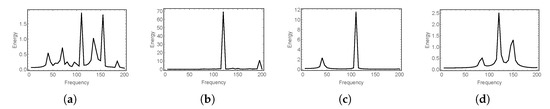
Figure 8. Frequency response: Regular penetration pattern and isotropic material. Loading $\widehat{f}(x,y)=1000cos\left(Ky\right)$. Cases: (a) parabolic: $K=1/2$; (b) hyperbolic: $K=1/2$; (c) parabolic: $K=4$; (d) hyperbolic: $K=4$.

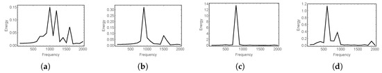
Figure 9. Frequency response: Regular penetration pattern and isotropic material. Loading is adapted to the penetration pattern for a special effect. Despite the symmetric configuration, the responses depend on the phase of the loading. Cases: (a) parabolic: $\widehat{f}(x,y)=1000cos\left(20y\right)$; (b) parabolic: $\widehat{f}(x,y)=1000sin\left(20y\right)$; (c) hyperbolic: $\widehat{f}(x,y)=1000cos\left(20y\right)$; (d) hyperbolic: $\widehat{f}(x,y)=1000sin\left(20y\right)$.

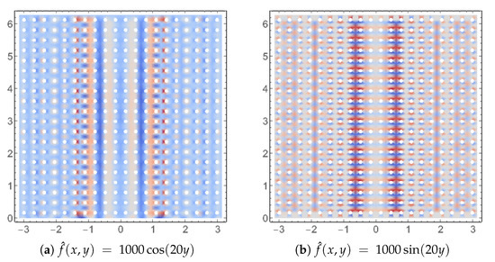
Figure 10. Hyperbolic: Grid adapted loading; Transverse deflections (w component) of the solutions with highest energies. Cosine case has maximal loads on the perforations whereas sine has minimal. Corresponding energies have an order of magnitude difference (see Figure 9).

The frequency response graphs show typical resonance patterns. The responses clearly depend not only on the loading, but also on the shell geometry. The observed maximal energies differ considerably, and, for a fixed frequency interval with $K=1/2$, the highest one is hyperbolic, but with $K=4$ parabolic.

5.2. Effect of the Random Material Parameter

In the second experiment, we let the Young’s modulus be random. We let $M=3$, and use full three point Gaussian quadrature in all stochastic dimensions. Thus, the associated collocation operator is given by (33) with the multi-index set $\mathcal{A}=\{\alpha \in {\mathbb{N}}_0^M|{\alpha }_m\le 2,m=1,\dots ,M\}$ and every example consists of 27 separate experiments covering the frequency range, now reduced to $\omega =2\pi f$$\mathrm{Hz}$, $f=30,40,\dots ,130$. Due to increased computational cost, we lower the polynomial order to $p=3$ in all remaining experiments.

The analysis of the results can now be performed on two levels, either by collocation or by sample statistics. Indeed, these results are very close, but of course not the same. See Figure 11 and Figure 12. We can take one step further and compute higher moments and even plot them. In Figure 13 and Figure 14, we show two solutions (expected solutions) with highest energies and their respective variances, one on a regular grid and another one on the Halton grid. Notice that for both geometries the variances in the regular grid cases reflect the fact that the random material parameter depends only on the axial direction.

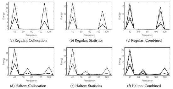
Figure 11. Parabolic: Expected frequency response and one standard deviation; Random material parameter. Top row: Regular grid; Bottom row: Halton grid. Solid line, expected response; Dashed line, expected response with one standard deviation added; Dot-dashed line, sample mean; Dotted line, sample mean with sample based standard deviation added.

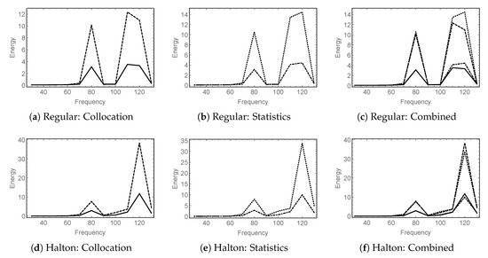
Figure 12. Hyperbolic: Expected frequency response and one standard deviation; Random material parameter. Top row: Regular grid; Bottom row: Halton grid. Solid line, expected response; Dashed line, expected response with one standard deviation added; Dot-dashed line, sample mean; Dotted line, sample mean with sample based standard deviation added.

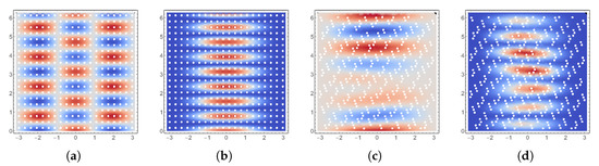
Figure 13. Parabolic: Random material; Transverse deflections (w component) of the solutions with highest energies. Expected solution and variance are computed using collocation; (a) and (b) on regular grid; (c) and (d) on Halton grid.

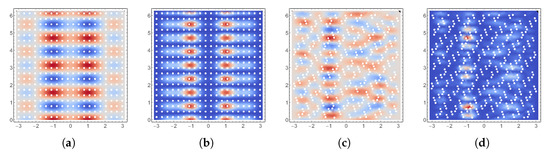
Figure 14. Hyperbolic: Random material; Transverse deflections (w component) of the solutions with highest energies. Expected solution and variance are computed using collocation; (a) and (b) on regular grid; (c) and (d) on Halton grid.

In Figure 14c, the response on the Halton grid is shown in the hyperbolic case. Interestingly, the irregular grid leads to a response that has an approximate angular wave number $K_H=7$, even though the excitation has $K=4$. This is an example where it is very difficult to predict the number of modes for the subspace if one wanted to apply some reduced basis method. In Table 3, we see that in the hyperbolic case the lowest modes are in a tight cluster and therefore it is likelier than in the parabolic case that perturbations result in higher order responses.

5.3. Effect of Local Low Intensity Damage

Next, we only perturb the penetration pattern using the damage model described above. Here, two interesting events can take place. It can happen that the damaged model leads to a response that is a close approximation of one the eigenmodes. An example of this is shown in Figure 15b,c. On the other hand, the damage may be close to the boundary and the associated boundary layer can result in local high energy feature in the response.

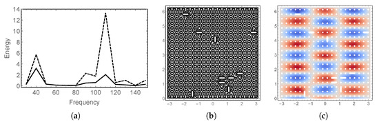
Figure 15. Parabolic: Damage model; Cases: (a) frequency response; (b) and (c) mesh and transverse deflection of the case with highest energy, respectively.

In Figure 15a and Figure 16a, the standard response profiles are shown. Again, a rare, but significant response is indicated with a large standard deviation (i.e., large variance). In Figure 15a, we see that the important frequencies are $f=40$ and $f=110$. We interpret the differences in the responses at the two frequencies so that it is likelier that there is a response at $f=40$, but at $f=110$ a very energetic response is possible but rare.

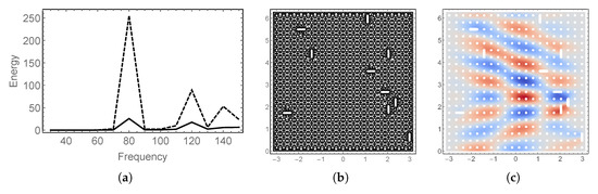
Figure 16. Hyperbolic: Damage model; Cases: (a) frequency response; (b) and (c) mesh and transverse deflection of the case with highest energy, respectively. Notice the internal boundary layers along the characteristics of the surface.

Of particular interest is the hyperbolic case of Figure 16c. Even though the loading is constant in the axial direction and periodic in the angular, the transverse deflection clearly shows internal layers (refer to Figure 7 above). The damaged holes perturb the regular pattern and generate internal layers which travel along the characteristics of the surface. Since the shells are surfaces of revolution, the characteristic lines align themselves close to the boundary. In fact, a similar phenomenon occurs for the parabolic case in Figure 15c but is obscured by the effect of the axially aligned loading.

5.4. Hybrid Uncertainty

Finally, we consider the full model where both the material parameter and the damage are included in the uncertainty quantification. Since the damage model does not preserve the symmetries, it follows that the variances of the highlighted solutions do vary over the whole domain and the structure of for instance Figure 13a is not preserved.

In the spirit of Algorithm 1, we simulate $S=100$ damage models each with a random material parameter as above leading to 2900 solutions per geometry type. The frequency responses and highlighted cases are given in Figure 17 and Figure 18. Again, the internal boundary layers are clearly visible in the transverse deflections, and even in the variance plots as well!

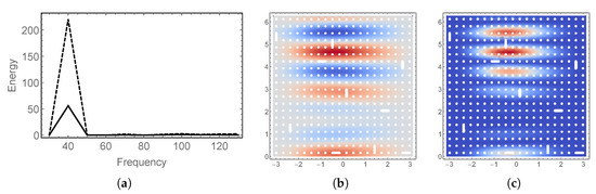
Figure 17. Parabolic: Damage model with random material; Cases: (a) frequency response; (b) and (c) expectation and variance of the transverse deflection of the case with highest energy, respectively.

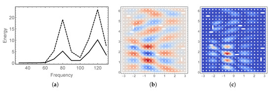
Figure 18. Hyperbolic: Damage model with random material; Cases: (a) frequency response; (b) and (c) expectation and variance of the transverse deflection of the case with highest energy, respectively. Notice the internal boundary layers along the characteristics of the surface.

In Figure 19, the energy distributions at the frequencies where the most energetic cases occur are shown. The distributions are exponential, which makes design of reliable damage detection algorithms challenging. However, this underlines the fact that comprehensive statistical understanding of the problem class is required, and systematic use of the stochastic finite element method and related techniques is well motivated.

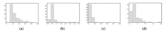
Figure 19. Energy distributions of the expected solutions ${\mathbb{E}}_{\mathsf{\Gamma }}\left[\widehat{\mathbf{v}}\right]$ for each of the 100 different simulations of the damage model. Cases: (a) and (b) parabolic samples at $f=40$ and 110, respectively; (c) and (d) hyperbolic samples at $f=80$ and 120, respectively.

6. Conclusions

For perforated shell structures, frequency response analysis is complicated by the wide range of parameters affecting the results. Indeed, shell is not referred to as the primadonna of structures for nothing. For instance, one has to have a good a priori understanding of the boundary layer structure, since, for sufficiently thin shells, the local features dominate and the damage detection algorithm has to be selected or tuned accordingly.

In general cases, any successful homogenization procedure should be able to match the subspaces between the perforated and non-perforated configurations. At the moment, solutions to this problem are at least as complex as direct simulations, which is the approach chosen here. Adding material uncertainties and simple damage models makes this problem even harder to resolve. In specific cases where the relevant parameters and their ranges can be reliably identified, homogenization can be accomplished with less effort.

Nevertheless, the simulations indicate that statistical and/or probabilistic modeling techniques are likely to be the best candidates for widely applicable damage detection methods in this context. Through reliable computations, it is possible to establish good approximations to distributions of the quantities of interest. The computational methodology advocated here can be used to build statistical databases that are necessary for development of probabilistic damage identification algorithms.

References

- Carden, E.P.; Fanning, P.; Carden, E.P.; Fanning, P. Vibration based condition monitoring: A review. J. Struct. Health Monit. 2004, 3, 355–377. [Google Scholar] [CrossRef]
- Fan, W.; Qiao, P. Vibration-based Damage Identification Methods: A Review and Comparative Study. Struct. Health Monit. Int. J. 2011. [Google Scholar] [CrossRef]
- Martikka, H.; Taitokari, E. Design of perforated shell dryings drums. Mech. Eng. Res. 2012, 2. [Google Scholar] [CrossRef]
- Jhung, M.J.; Jo, J.C. Equivalent material properties of perforated plate with triangular or square penetration pattern for dynamic analysis. Nucl. Eng. Technol. 2006, 38, 689–696. [Google Scholar]
- Jhung, M.J.; Yu, S.O. Study on modal characteristics of perforated shell using effective Young’s modulus. Nucl. Eng. Des. 2011, 241, 2026–2033. [Google Scholar] [CrossRef]
- Jhung, M.J.; Jeong, K.H. Free vibration analysis of perforated plate with square penetration pattern using equivalent material properties. Nucl. Eng. Technol. 2015, 47, 500–511. [Google Scholar] [CrossRef]
- Korea Institute of Nuclear Safety. Free Vibration Analysis of Perforated Cylindrical Shell Submerged in Fluid; Technical Report, KINS/RR-493; Korea Institute of Nuclear Safety: Daejeon, Korea, 2007. [Google Scholar]
- Hakula, H.; Laaksonen, M. Multiparametric shell eigenvalue problems. Comput. Methods Appl. Mech. Eng. 2019, 343, 721–745. [Google Scholar] [CrossRef]
- Hakula, H.; Kaarnioja, V.; Laaksonen, M. Cylindrical Shell with Junctions: Uncertainty Quantification of Free Vibration and Frequency Response Analysis. Shock Vib. 2018, 2018, 5817940. [Google Scholar] [CrossRef]
- Szabo, B.; Babuska, I. Finite Element Analysis; Wiley: Hoboken, NJ, USA, 1991. [Google Scholar]
- Schwab, C. p- and hp-Finite Element Methods; Oxford University Press: Oxford, UK, 1998. [Google Scholar]
- Chapelle, D.; Bathe, K.J. The Finite Element Analysis of Shells; Springer: Berlin/Heidelberg, Germany, 2003. [Google Scholar]
- Malinen, M. On the classical shell model underlying bilinear degenerated shell finite elements: General shell geometry. Int. J. Numer. Methods Eng. 2002, 55, 629–652. [Google Scholar] [CrossRef]
- Forskitt, M.; Moon, J.R.; Brook, P.A. Elastic properties of plates perforated by elliptical holes. Appl. Math. Model. 1991, 15, 182–190. [Google Scholar] [CrossRef]
- Burgemeister, K.A.; Hansen, C.H. Calculating resonance frequencies of perforated panels. J. Sound Vib. 1996, 196, 387–399. [Google Scholar] [CrossRef]
- Halton, J.H. Algorithm 247: Radical-inverse Quasi-random Point Sequence. Commun. ACM 1964, 7, 701–702. [Google Scholar] [CrossRef]
- Pitkäranta, J.; Matache, A.M.; Schwab, C. Fourier mode analysis of layers in shallow shell deformations. Comput. Methods Appl. Mech. Eng. 2001, 190, 2943–2975. [Google Scholar] [CrossRef]
- Ghanem, R.; Spanos, P. Stochastic Finite Elements: A Spectral Approach; Dover Publications, Inc.: Mineola, NY, USA, 2003. [Google Scholar]
- Inman, D.J. Engineering Vibration; Pearson: London, UK, 2008. [Google Scholar]
- Babuška, I.; Nobile, F.; Tempone, R. A stochastic collocation method for elliptic partial differential equations with random input data. SIAM J. Numer. Anal. 2007, 45, 1005–1034. [Google Scholar] [CrossRef]
- Nobile, F.; Tempone, R.; Webster, C.G. An Anisotropic Sparse Grid Stochastic Collocation Method for Partial Differential Equations with Random Input Data. SIAM J. Numer. Anal. 2008, 46, 2411–2442. [Google Scholar] [CrossRef]
- Bieri, M. A Sparse Composite Collocation Finite Element Method for Elliptic SPDEs. SIAM J. Numer. Anal. 2011, 49, 2277–2301. [Google Scholar] [CrossRef]
- Andreev, R.; Schwab, C. Sparse Tensor Approximation of Parametric Eigenvalue Problems. In Lecture Notes in Computational Science and Engineering; Springer: Berlin, Germany, 2012; Volume 83, pp. 203–241. [Google Scholar]
© 2019 by the authors. Licensee MDPI, Basel, Switzerland. This article is an open access article distributed under the terms and conditions of the Creative Commons Attribution (CC BY) license (http://creativecommons.org/licenses/by/4.0/).