Stressing State Analysis on a Single Tube CFST Arch Under Spatial Loads

Abstract

This paper analyzes the stressing state characteristics of a concrete-filled steel tubular (CFST) arch model under spatial loads, using the method of modeling structural stressing state and the thin plate simulating interpolation (TSI) method. Firstly, the parameter-generalized strain energy density (GSED) is applied to model the stressing state of the arch. Then, the normalized GSED sum at each load plots the characteristic curve. The characteristic loads P (66 kN) and Q (85 kN) in the curve are distinguished by the Mann–Kendall (M–K) criterion. To characterize structural axial and bending stressing states, the parameters of the sectional average strain and generalized bending strain are proposed as stressing state submodes. Finally, the TSI method is used to interpolate strain data for deep analysis of internal forces. By modeling the structural stressing state, the working behavior characteristics of arch structures are greatly revealed in a particular view and the results could provide a reference for the development of bridge design.

1. Introduction

Concrete-filled steel tubular (CFST) arches, which consist of thin-walled steel tubes and concrete cores, are gaining more and more popularity in bridge construction because of their high bearing capacity, light self-weight, and convenient construction [1,2]. The thin-walled steel tube could provide effective confinement for the concrete core and significantly improve its compressive performance and ductility; meanwhile, the concrete core can also provide restraint to improve the local buckling of the steel tube [3]. Therefore, CFST arches are considered good alternatives for reinforced concrete bridges or steel arch bridges. The well-bonded steel tube and concrete core composite cross section can provide enough structural stiffness and strength in practical application. Furthermore, the steel consumption can be minimized to reduce project cost [4]. The composite members have hitherto been constructed throughout the world with rapid development because of the mutual promotion between concrete and steel tubes [5,6]. Especially in China, more than 400 CFST arch bridges have been built or are currently under construction [7].

As the development of CFST arches is fast-growing, the working behavior of CFST arches is of more and more concern. Over the last 20 years, many researchers have paid attention to the in-plane stabilities of CFST arches and obtain important achievements. Theories and methods were proposed to investigate the stability of arches. Furthermore, experimental analysis were conducted [8,9,10,11,12]. Some simplified formulas were also proposed to evaluate the load-bearing capacity of arch bridges [13].

As for out-plane stability of the CFST arches, research findings are quite limited. Lin [14] carried out the experimental study on a CFST (single tube) arch with one rib under spatial loads and laid the foundation for future research on the spatial load-carrying capacity of CFST arches. Chen et al. [15] used the finite element (FE) method to carry out the dual non-linearity analyses for CFST arches with a single rib under spatial loads and found that the influence of geometric nonlinearity increased, compared to arches under in-plane loads. Li [16] analyzed the out-plane stability of CFST arches and proposed corresponding design formula. Deng et al. [17] established a co-rotational formulation in the setting of finite elements for three-dimensional nonlinear analysis of ultimate bearing capacity of a circular CFST arch subjected to in-plane and out-plane loads, considering both geometric and material nonlinearities. Wang et al. [18] analyzed the out-plane elastic stability of typical tube CFST arch bridge by FE method, and the results indicate that the FE model, based on the statistical data, could reflect the working performance of the structure. Yang et al. [19] presented a self-adaptive method of elastic modulus reduction to evaluate the ultimate load bearing capacity of CFST arch bridges. Geng et al. [20] proposed designing equations on the basis of the FE analysis to predict the ultimate loads of CFST arches.

As noted, the limited research in the open literature indicates that there are a shortage of sufficient large-scale experiments on CFST arches to analyze the complex out-plane working behaviors and instability mechanisms [21]. The high experimental cost confines the development of research to some degree. Furthermore, the experimental data are always not fully utilized, leading to the negligence of extensive unseen information of structural working behavior characteristics. It is significant to use appropriate methods to analyze the working behavior of CFST arches on the basis of existing experimental data. Besides, in the simulation analysis, the FE models are simplified on the basis of assumptions. Consequently, the calculation results are deficient in universality and conservative in application, leading to the overuse and/or irrational use of materials.

All these problems indicate that the existing theories/methods cannot completely reveal the working characteristics hidden in CFST arches and new methods are required. On the basis of the analysis on CFST arches under in-plane loads [22], this paper reveals the working characteristics of a single tube CFST arch model under spatial loads, applying the method of modeling structural stressing state. By adopting the parameters of the generalized strain energy density (GSED), the stressing state mode of the arch is characterized. The Mann–Kendall (M–K) criterion is then used to distinguish the characteristic loads. Using the thin plate simulating interpolation (TSI) method, the stress/strain fields and internal forces of the arch are obtained to further analyze the structural behavior.

2. Method of Modelling Structural Stressing State

2.1. Modelling of Structural Stresing State

The stressing state mode of the one arch structure is the numerical description of the working behavior characterized by structural responses. Strains and stress can reflect the working behavior and deformation of the structure. From this angle, the generalized strain energy density (GSED) [23,24], a microcosmic scalar relating to strain and stress, can be used to describe the stressing state of the arch. Although other structural response parameters, such as strains and displacements, can also embody the inner or outer working characteristics under loads, they are considered limiting.

For one measured point of the arch structure, its GSED value can be expressed as

$$E_{ij}={\displaystyle {\int }_0^{{\epsilon }_{ij}}\sigma \mathrm{d}\epsilon },$$

(1)

where E_ij is the GSED value of i-th point under j-th load; ε_ij is the strain value measured at this point. To calculate the stressing state of the entire structure or some segments of the whole (components, joints, etc.), GSED values of all concerned points should be summed, that is

$$E_j={\displaystyle \sum _{i=1}^n{E}_{ij}},$$

(2)

where E_j is the GSED sum of all related points, n is the total number of points. By use of a dimensionless process, the GSEDs are normalized as the dimensionless physical quantity E_j,norm to characterize the distribution mode of the stressing state, that is

$$E_{j,\mathrm{norm}}=\frac{E_j}{E_{\max }},$$

(3)

where E_max is the maximum GSED sum throughout the loaded process. Thus, all these E_j,norm values are assembled with load F_j as the numerical mode to plot the E_j,norm-F_j (denoted as E-F for convenience) curve and calculate the working characteristics of the arch.

2.2. The Application of Mann–Kendall Criterion

According to the natural law that the evolution of a system always requires a course of gradual accumulation, and one from quantitative to qualitative changes, the working behaviors of a structure subjected to certain loads are bound to evolve with load increasing and reflect different stressing state characteristics at different loading stages [25,26]. As long as the load reaches a certain level, the structural stressing state may present the qualitative leap characteristic from the quantitative change. This certain load indicates that from then on, the structure exists great potential safety hazard and is unsuitable for load bearing. As a trend analysis tool in hydrometeorology, the Mann–Kendall (M–K) criterion [27,28,29] is found to detect well the leap characteristics from the E-F curve [22].

It is assumed that the sequence of {E_j,norm} (the load step j = 1, 2, …, n) is statistically independent. For the sequence {E_j,norm}, the cumulative number m_i is taken if E_i,norm is greater than E_j,norm (1 ≤ j ≤ i). We define a new stochastic variable q_k at k-th load step (2 ≤ k ≤ n) by

$$q_k={\displaystyle {\sum }_{i=1}^k{m}_i}.$$

(4)

The mean value E(q_k) and variance V(q_k) are calculated, they are

$$E(q_k)=k(k-1)/4,$$

(5)

$$V(q_k)=k(k-1)(2k+5)/72.$$

(6)

Then, a new statistic UF_k is defined by

$$U{F}_k=\{\begin{array}{ll}0& k=1\\ \left(q_k-V(q_k)\right)/\sqrt{V(q_k)}& 2\le k\le n\end{array}.$$

(7)

For all the UF_k data, it can form the UF-F curve. A similar procedure is proceeded to the inverse sequence {E_j,norm} to calculate another statistic UB_k and form the UB-F curve. Consequently, the intersecting point of the UF and UB curves is the characteristic load of the E-F curve.

3. Introduction of the Experiment

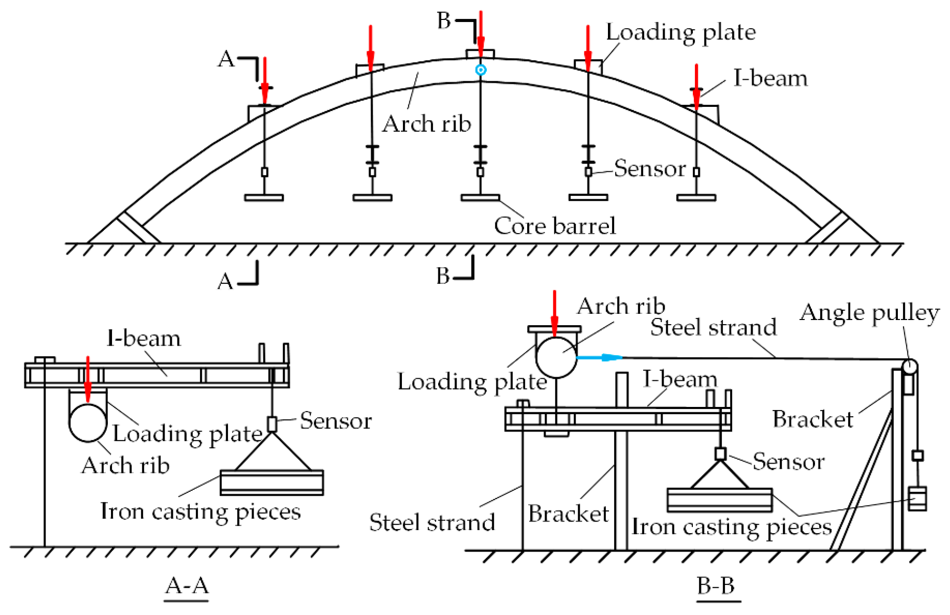
3.1. Test Setup

Chen [15] conducted the experiment of a parabolic single tube CFST arch subjected to spatial loads in the lab of Fuzhou University. The model arch was 7.5 m in span, 1/5 rise-span ratio, 121 mm in diameter and 4.5 mm in thickness of steel tube. The yield stress, elastic modulus of steel and cubic compressive strength, elastic modulus of concrete were 322 MPa, 206 GPa and 66.7 MPa, 35.6 GPa, respectively.

As shown in Figure 1, the experimental loading apparatus was fabricated to apply horizontal and vertical loads simultaneously. Five sets of loading apparatus were set at equal intervals along the arch span respectively to apply in-plane point loads, and a set of horizontal loading devices was arranged at arch vault to apply the out-plane point load. For applying vertical loads, lever method was adopted to enlarge the gravity action of iron casting pieces, as shown in the A-A profile. A fixed pulley was used to transform gravity action into a horizontal point load, as shown in the B-B profile.

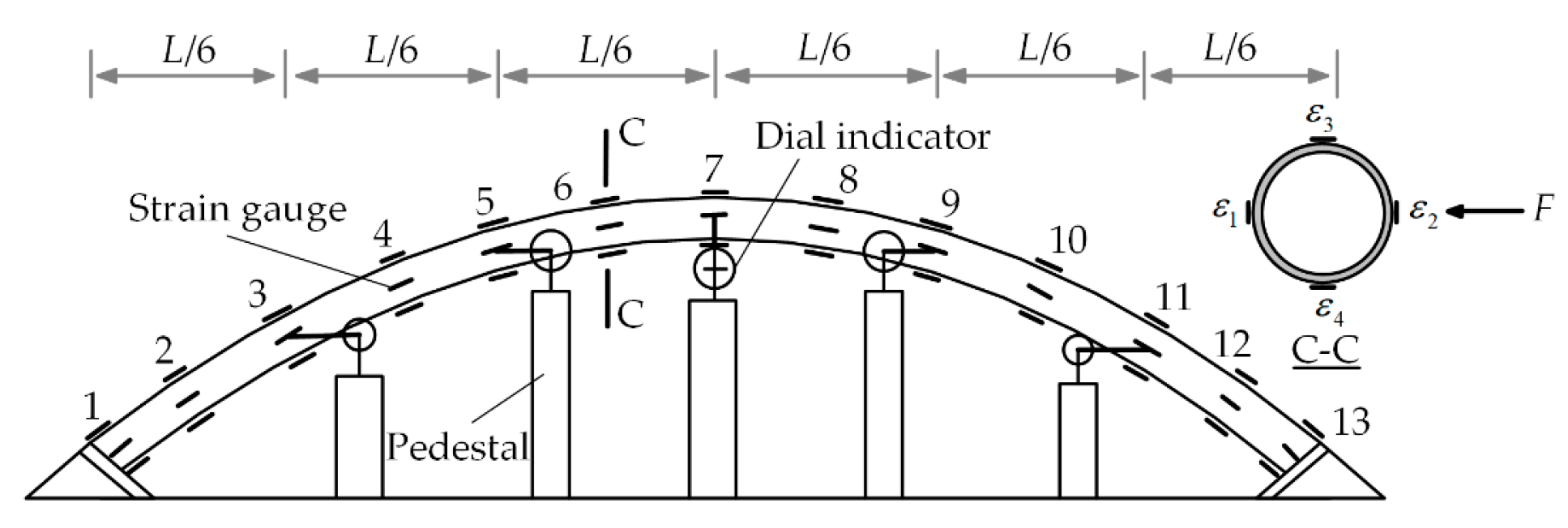
3.2. Test Scheme

As shown in Figure 2, in total, thirteen measuring sections 1–13 were set equally spaced along the arch span. Around each section, four strain gauges (numbered from ε₁–ε₄) were placed on the outer surface of the steel tube to monitor longitudinal strains. Besides, dial indicators were distributed at spans L/6, L/3, L/2, 2L/3 and 5L/6 (Sections 3, 5, 7, 9, 11 and 13) to record both horizontal and vertical displacements.

During the loading process, in-plane vertical loads and out-plane load were simultaneously loaded to simulate the process of spatial loads. By employing step loading, vertical loads increased 10 kN at each load level before 30 kN and then 5 kN until 60 kN. After 60 kN, each load level was 2.5 kN until the instability of the arch model at 97 kN. The value of the horizontal load was applied at 10% of the vertical load each time, so that the load F in the paper represents the value of vertical loads without an additional description of horizontal loads.

4. Stressing State Analysis of the Arch Model

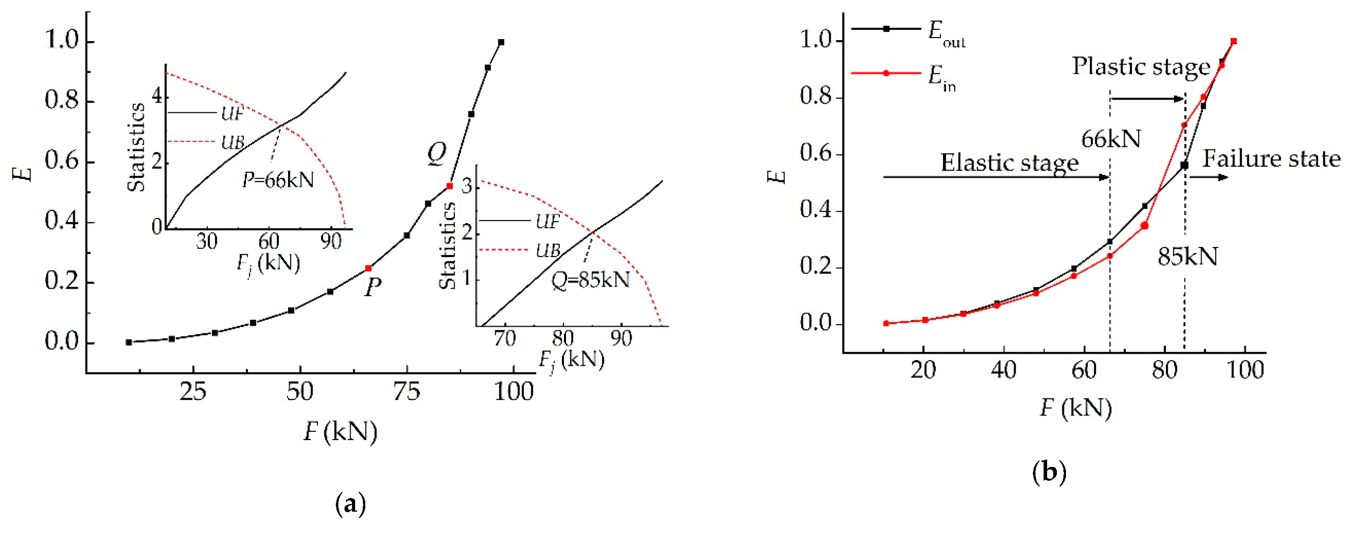
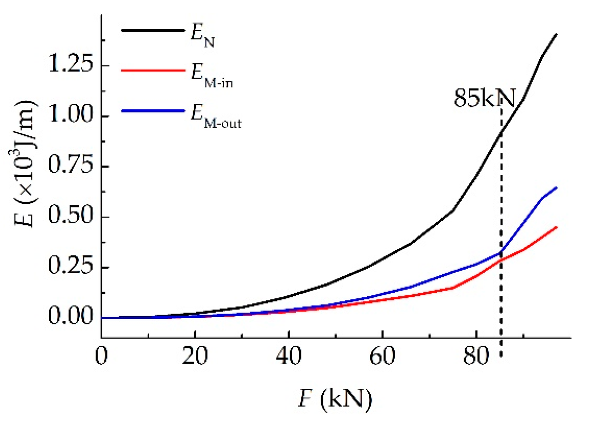
4.1. Investigation into the E-F Curve

By calculating GSED values with strains of each measured point according to Equations (1)–(3), it can directly model the stressing state mode of the arch under spatial loads. Thus, the E-F curve is plotted to describe the working characteristics of the arch model during the whole loading process, as shown in Figure 3a. To distinguish the first characteristic load in the curve, the M–K criterion is applied to achieve the intersecting point of the UF and UB curves based on the sequence of {E_j,norm} from 0 kN to 97 kN. As for the second characteristic load, the sequence {E_j,norm} is from 66kN to 97 kN. Hence, two characteristic loads, P (66 kN) and Q (85 kN), are obtained. According to the two loads, the structural stressing state curve of the arch model is directly divided into three different stages. Before load P, the curve presents steady changes with load increase, indicating that the arch is basically in the linear-elastic working state in this stage. After load P, the arch model is in the elastic-plastic working state due to the local plastic development of steel tube. According to the natural law from quantitative change to qualitative change, characteristic load Q is detected, whereas thereafter a trend of relatively sharper increase of the E emerges and the arch enters the unstable working state until its finally failure at ultimate load (97 kN).

Since the arch model is subjected to in-plane and out-plane loads simultaneously, the formation of strains ε₁, ε₂ and ε₃, ε₄ are considered the action results of both axial forces but out-plane and in-plane bending moments, respectively. Thus, the strains ε₁, ε₂ and ε₃, ε₄ of one section can be normalized as the out-plane and in-plane GSED values, respectively, to observe their stressing state characteristics. When calculating the value of out-plane GSEDs (E_out) by Equations (1)–(3), only ε₁ and ε₂ of each cross section are considered, similarly, we consider strains ε₃, ε₄ only to calculate the in-plane GSEDs (E_in). Therefore, the E-F curves for out-plane and in-plane ones can be plotted, as illustrated in Figure 3b. From loads P to Q, the E_in-F curve has an obvious change at 75 kN, while the E_out-F curve keeps a normal increase. At 85 kN, E_out has an obvious change (turning point) together with a little trend change of E_in. It seems that the in-plane and out-plane working behaviors are relatively independent before load P (66 kN); but from loads P to Q (85 kN), the in-plane and out-plane working behaviors could be coupled with each other. After point Q, the whole arch is in failure state controlled by out-plane behaviors.

According to the investigation above, two common characteristics are summarized to describe the stressing state of the arch model. Firstly, characteristic load P is the branch point that the stressing state of the arch changes from elasticity to elastoplasticity. The whole structure keeps a stable stressing state until load Q. In other words, the arch’s stressing state keeps quantitative change rather than qualitative change. Secondly, characteristic load Q is the branch point where the arch’s stress state qualitatively changes/leaps to an unstable stressing state state that is different from before. Hence, the load at point Q is defined as the failure load of the arch structure to represent the starting point of structural failure process. It is the essential and general working behavior characteristic that arch structures certainly present during their loading process. This certain load indicates that from then on, the structure presents a great, potential safety hazard and is unsuitable for load bearing. The updated failure load just matches this certain load, and the following sections further investigate the characteristics of structural stressing state modes formed by GSED values and internal forces. To make a distinction, the present failure load we defined at the ultimate load is the load that the structures have already been destroyed.

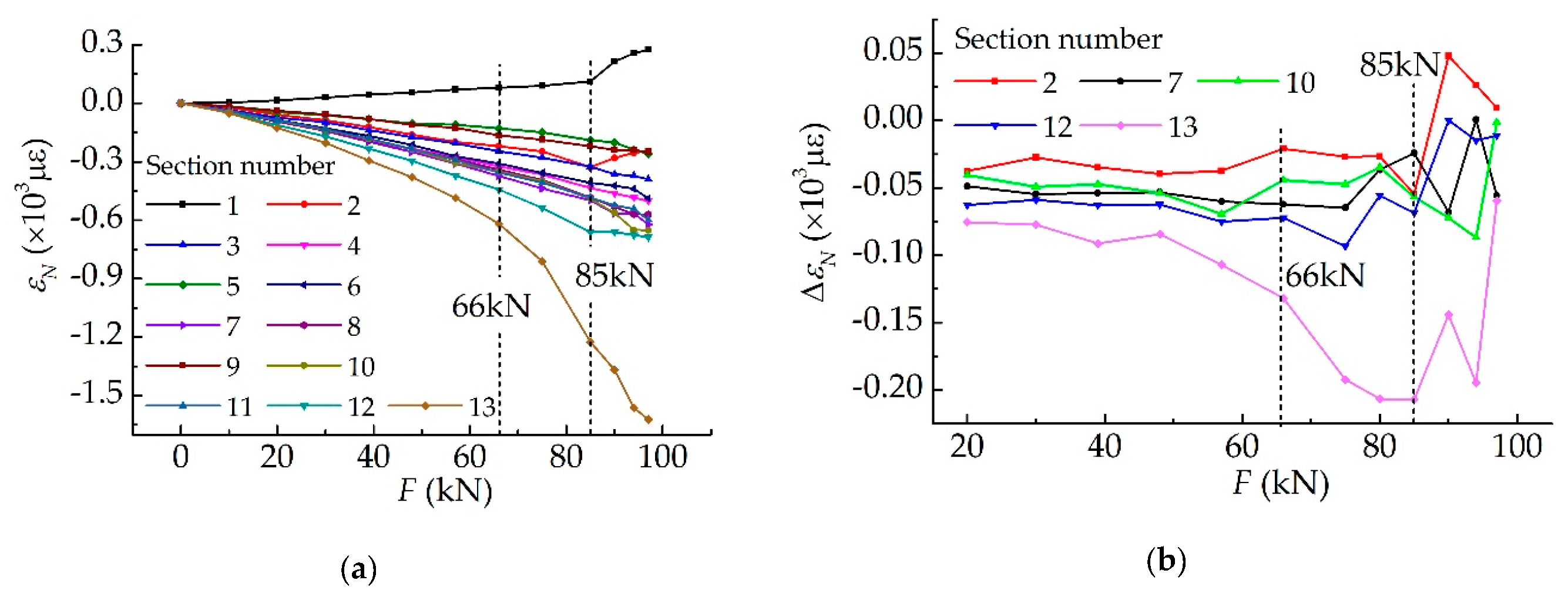
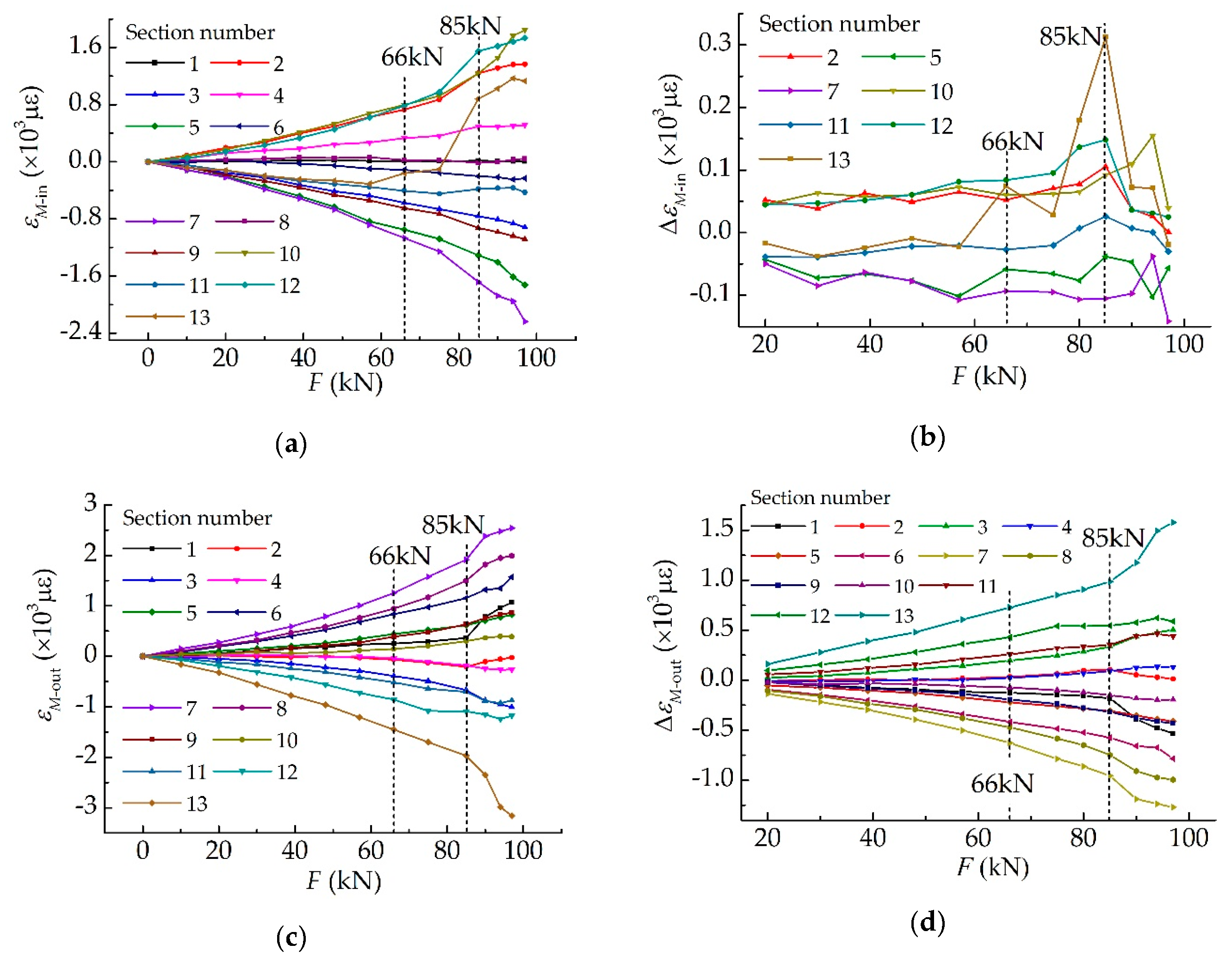
4.2. Characteristic Investigation into Strains

Strains can reflect the working state of the structure to some extent. Thus, by modelling the experimental strains at typical sections, it can reflect the internal working behavior characteristics of the arch model. Here, the GSED sum of each cross section are adopted to describe the stressing state of one section, that is

$$E_j=E_1+E_2+E_3+E_4,$$

(8)

where E_j is the GSED sum of the cross section under j-th load, E₁~E₄ are GSEDs calculated by strains ε₁~ε₄ under the j-th load, respectively.

As shown in Figure 4a, the E_j-F curves of each cross section are plotted to reflect the change trend of the structural stressing state mode. It can be seen that before 66 kN, E_j at all these sections keeps a slight and stable increase with no sharp break between adjacent loads. From then on, with the increasing of loading, E_j at some sections embody greatly faster increasing trends than other sections, especially sections at the arch foot and mid-span (Sections 7 and 13). The larger the E_j is, the greater the stress the cross section has. Therefore, it indicates that these zones, around Sections 7 and 13, are the weak parts of the arch, which controls the arch’s instability failure during the later part of the loading application. Besides, the asymmetry of the E_j-F curves at symmetrical sections also embodies the effect of many factors, such as uncertainties in the experiment, both geometrical and material nonlinearities. Even so, the developing trend of the curves would not be changed and have a good presentation of mutation characteristics of the stressing state mode.

To better view the change trend of the E_j-F curves, the increment difference of E_j between adjacent loads are modelled as the characteristic parameter ∆E_j, that is

$$\Delta E_j=E_j-E_{j-1}.$$

(9)

As shown in Figure 4b, the ∆E_j-F curves of some typical sections are plotted. It shows that curves of some sections, like Sections 1 and 3, have little increments during the whole load process, and the fluctuating ranges of these curves are not obvious enough after 85 kN. By comparison, the curves of typical sections, like Sections 7 and 13, show an obvious increasing trend from 66 kN to 85 kN and great increments after 85 kN, illustrating the important qualitative change of stressing the state mode of the arch model. Hence, from the perspective of experimental strains, it can evidently embody the leap change of the arch’s stressing state mode after the failure load.

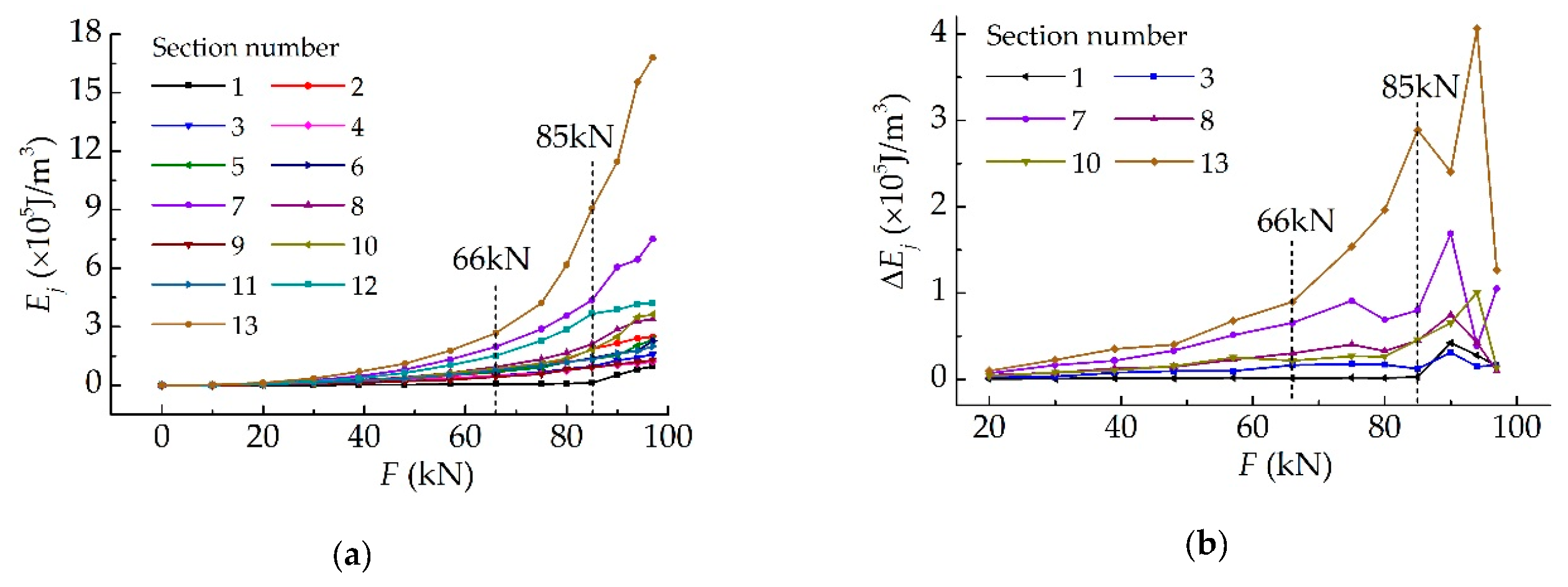
4.3. Modelling of Stressing State Submodes

As for the internal forces of the arch model, it withstands axial force, bending moment, and torsion under spatial loads. Due to the little effect of torsion, it can be ignored in analysis [14]. Thus, the stressing state mode of the arch can be mainly decomposed into stressing state submodes for axial compression and the bending moment, respectively, to characterize their working behavior and illustrate their different roles in the loading process.

Longitudinal strains measured around each cross section are the most direct reflection of axial force. However, the strains of separate points have high variability and low determinacy, so they could not accurately judge the stressing state submode for axial compression. Therefore, the mean value of sectional strains is calculated as a quantitative index, called the “axial strain” ε_N, to represent the action effect of axial compression at the sectional centroid point, that is

$${\epsilon }_N=\frac{1}{4}({\epsilon }_1+{\epsilon }_2+{\epsilon }_3+{\epsilon }_4).$$

(10)

Thus, the ε_N of all these sections can be calculated to embody the developing trend of the stressing state submode for the axial force. To better observe the increasing trend of ε_N between adjacent loads, the difference value ∆ε_N is also calculated.

As shown in Figure 5, the stressing state submode for axial forces and the increasing trend of some typical sections are plotted. It shows that the curves are divided into three different developing trends. Before 66 kN, the ε_N increases slowly with no obvious mutation; during 66 kN to 85 kN, the ε_N of some sections increase rapidly; after 85 kN, the curves signify the unstable stressing state. Due to the sensitivity of the arch foot, the ε_N shows great values at Section 13. Besides, the axial forces in the arch appear as compression under normal circumstances, so the ε_N should be negative normally. But it is found in Figure 5a that the ε_N present positive at Section 1, while other sections are all negative. This may be caused by an inaccuracy in the measurement or by the geometric and material nonlinearity of the arch, whereby local buckling of steel tube may also be produced.

Compared to the submode for axial force, the stressing state submodes for bending moments of the arch model come into greater focus. Similar to the construction of ε_N, sectional strains are applied to construct the parameter “generalized bending strain” ε_M, to quantitatively describe the submodes for bending moments. Under spatial loads, the bending moments can be decomposed into in-plane bending moments and out-plane ones. Hence, the strains ε₁, ε₂ and ε₃, ε₄ are divided to calculate the out-plane ε_M-out and in-plane ε_M-in , respectively, they are

$${\epsilon }_{M-\mathrm{out}}=\frac{1}{2}({\epsilon }_1-{\epsilon }_2),{\epsilon }_{M-\mathrm{in}}=\frac{1}{2}({\epsilon }_3-{\epsilon }_4).$$

(11)

Thus, the ε_M of all these sections are calculated to embody the distribution of stressing state submodes for in-plane or out-plane bending moments. To better observe their growth trend between adjacent loads, the differences ∆ε_M-out or ∆ε_M-in are also calculated.

Figure 6 shows the changing features of the arch model’s stressing state submodes for bending moments, as well as the corresponding characteristic parameters ∆ε_M-out and ∆ε_M-in. Before 66 kN, the developing trends of both ε_M-in and ε_M-out are stable with light undulation. The obvious leap at about 75 kN (before failure load at 85 kN) in Figure 6a,b demonstrates that for the in-plane bending moment, the mutation characteristic may happen before failure load. This phenomenon is the same as the change characteristics embodied in Figure 3b. It can be seen from Figure 6c that the obvious increments after 85 kN greatly reflect the leap characteristic of the stressing state mode at failure load, especially the typical Sections 7 and 13.

Based on the elastic theory in a generalized sense, the energy densities per unit micro-segment corresponding to the axial and bending deformation forms are calculated by ε_N and ε_M, to approximately evaluate their contributions to the structural load-bearing behavior. Here, the energy-based characteristic parameters for axial force and bending moments (decomposing into in-plane and out-plane ones) are constructed, they are

$$E_N={\displaystyle \sum _{i=1}^m\frac{1}{2}N{\epsilon }_{Ni}}={\displaystyle \sum _{i=1}^m\frac{1}{2}EA{\left({\epsilon }_{Ni}\right)}^2},$$

(12)

$$E_M={\displaystyle \sum _{i=1}^m\frac{1}{2}M{\kappa }_i}={\displaystyle \sum _{i=1}^m\frac{1}{2}EI{\kappa }_i^2},{\kappa }_i=2\frac{{\epsilon }_{Mi}}{h},$$

(13)

where E_N and E_M are the arch’s generalized energy densities for axial force and bending moments, respectively; A and I mean cross-sectional area and moment of inertia, respectively; ĸ is curvature for cross section; m = 13 is the total number of cross sections.

Figure 7 illustrates the generalized energy densities for internal forces under loads. It shows that E_N corresponding to the effect of axial force are significantly higher than E_M-in or E_M-out, while the values of E_M-in and E_M-out are close to each other. Due to the weaker out-plane stiffness than the in-plane one, E_M-out have great values and effect the working behavior of the arch under small out-plane loads. Therefore, the failure of the arch is mainly controlled by out-plane factors, as well as the change characteristics embodied by them at failure load.

5. Stressing State Analysis Based on the Interpolation of Strains

The limited data of structural response collected from experiments can, to some extent, reflect the working behavior of the structure under loading, but, it cannot have a fully clear reflection of structural mechanical characteristics. By applying interpolation methods, more strain data can be obtained at non-sample points to have a more detailed reflection of the structural stressing state. However, the existing interpolation methods are almost on the basis of mathematical methods or statistical methods and lack clear physical meanings, leading to unsatisfactory interpolation results. Therefore, the authors propose the thin-plate simulating interpolation (TSI) method, with reference to the interpolation method of Thin Plate Splines (TPS) [22,30]. TSI applies the FE simulation of a specific thin-plate model to obtain the discrete weighting functions of sampled points. Then, the data at non-sampled points are acquired with the interpolation calculation of discrete weighting function and the sampled data. In addition, the interpolated smooth surface of TPS has the minimum bending energy, while that of TSI automatically possesses minimum potential energy (including bending energy). Hence, the interpolation results of TSI can reflect the deformation characteristics of the thin-plate more realistically, which is better to analyze the working behavior of the arch structure.

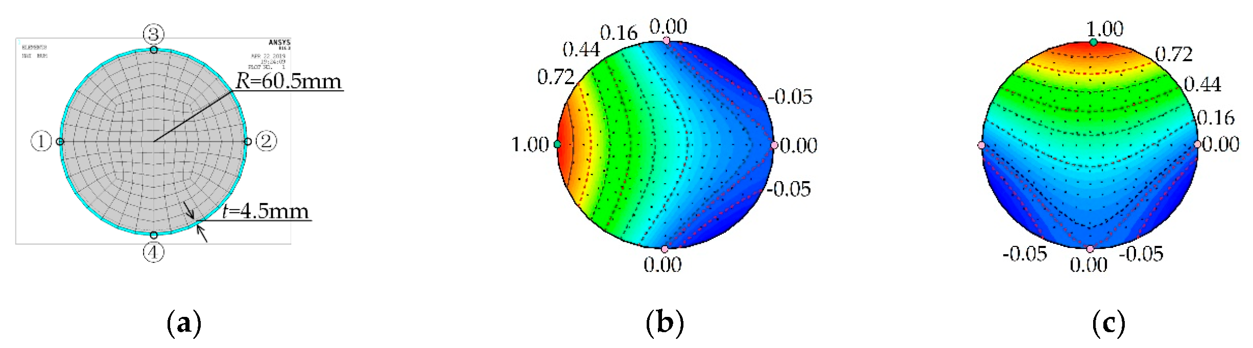
5.1. Interpolation of Strain/Stress Fields by TSI Method

First of all, the software ANSYS was used to construct the FE model of arch’s cross section and meshed the section model with element Shell 181, as shown in Figure 8a. The radius of the cross section (R) is 60.5 mm and the thickness of steel tube (d) is 4.5 mm. In the coordinate system (x,y), built in the FE model, the coordinate (x_j,y_j) corresponds to j-th element node. As known quantities, the deflections of controlled points 1~4 are correspondent with strains ε₁~ε₄. Similar to the calculation of common shape functions [31,32,33], the discrete weighting functions N₁~N₄ are obtained based on four controlled points. Take N₁ for example, applying a unit displacement at point 1 while points 2~4 are fixed to restrict rigid displacements, so N₁ is formed by static calculation and extracting the function values from each element node, as shown in Figure 8b. N₃ is also depicted in Figure 8c. Due to the central symmetry of the section shape, N₁ is in rotational symmetry with N₃.

The discrete weighting functions N₁~N₄ can be explained as the aggregations by all function values at element nodes, they are

$$N_i=\left[N_i(x_1,y_1),N_i(x_2,y_2),\cdots N_i(x_j,y_j),\cdots N_i(x_n,y_n)\right],$$

(14)

where N_i is the discrete weighting function acquired on the basis of i-th controlled point, N_i(x_j,y_j) is the function value at element node (x_j,y_j), n is the total number of element nodes. Without considering large deformation or elastoplasticity, the interpolation field constructed by Castigliano’s theorem is independent of loading paths, and linear superposition can be carried out for the simulative results with explicit physical meanings. Therefore, according to the deflection of points 1~4 and the corresponding discrete weighting functions N₁ ~ N₄, the deflection field D of the whole cross section is assembled, that is

$$D={\displaystyle \sum {\epsilon }_i{N}_i}.$$

(15)

In other words, D can be perceived as the aggregation of strains at all element nodes.

According to the constitutive relation of the materials, the corresponding stress filed is calculated. The constitutive models of concrete in compression and tensile behavior are the uniaxial stress-strain curve [34] and Gilbert’s model [35], respectively. As for steel, the five-stage stress-strain curve [36] is applied.

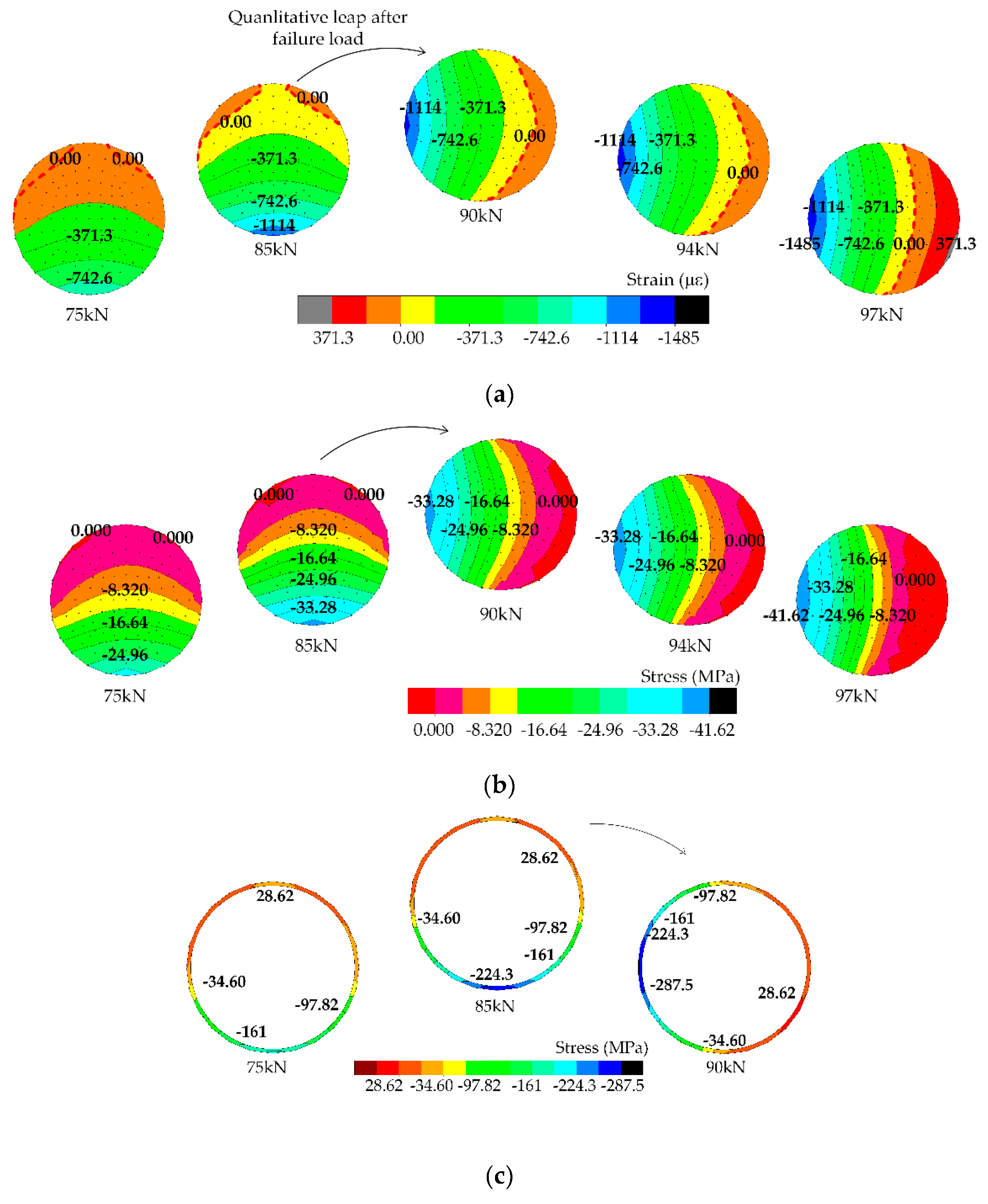
5.2. Analysis on Strain/Stress Fields

On the basis of the strain data measured in the experiment, strain/stress fields of all these 13 cross sections are constructed with the TSI method. Through the analysis of these strain/stress fields, some typical sections could show great change characteristics during loading. Here, Section 2 is chosen as an example to observe the characteristics of its strain/stress fields.

As shown in Figure 9, the strain/stress fields on Section 2 with different load levels around the failure load (85 kN) and at ultimate load (97 kN) are plotted. With load increasing, the maximum compressive/tensile strain increases while the tension zone decreases. When reaching the maximum load at 97 kN, the strain also reaches its maximum. It can be seen that the upper part of Section 2 is subjected to tension at 75/85 kN, and more than half the area is basically in the compressive state with small tensile strain values. After 85 kN, the left part of the cross section transforms into the tensile state. Obviously, the distribution shape of isopleth curves changes dramatically from one mode to another.

The similar regular pattern can be observed in Figure 9b,c. After the failure load at 85 kN, the distribution of stress changes essentially from one mode to another. Therefore, the obvious transformation after 85 kN adequately embodies the significant mutation of structural stressing state around the failure load.

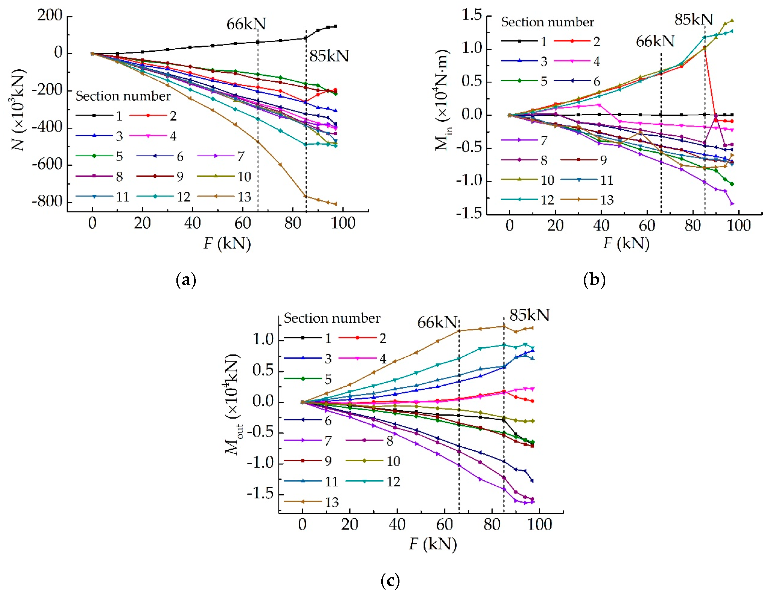
5.3. Analysis on Stressing State Submodes for Internal Forces

As mentioned above, the stressing state submodes for internal forces ε_N and ε_M can reflect the characteristics of structural working behavior qualitatively. However, due to the limit of strain data, it could not obtain the precise values of internal forces. Here, based on the interpolated strains of the whole cross section, it could have a rather accurate description of internal forces. By the quadrature method, internal forces of the cross section could be calculated, they are

$$N={\displaystyle {\int }_A\sigma \mathrm{d}A={\displaystyle \sum _A{\sigma }_i{A}_i}},$$

(16)

$$M_y={\displaystyle {\int }_A\sigma y\mathrm{d}A={\displaystyle \sum _A{\sigma }_i{y}_i{A}_i}},$$

(17)

where N and M_y are sectional internal forces of axial force and bending moment, respectively.

As shown in Figure 10, the developing trend of internal forces for axial force N and in-plane/out-plane bending moments M_in/M_out are plotted to reflect the changing characteristics of the stressing state submodes. Figure 10a shows that the maximum value of the axial force occurs at Section 13 with load increase, as well as great bending moments. Before 85 kN, the curves basically keep the growth trend unchanged while, thereafter, they change to another trend with obvious turning points. Besides, because of the initial geometrical imperfection (arch axis’s asymmetric deviation) of the arch, the distribution of F especially at arch feet is considerably asymmetrical. As for Figure 10b, in-plane bending moments show great values at arch vault and near arch feet with opposite directions. Some curves exhibit a little fluctuation and some others show the transition at 85 kN. As reflected in Figure 10c, the distribution of M_out shows the obviously essential change after 85 kN in some typical cross sections, e.g., Sections 3, 7, and 8.

Generally, the strain/stress fields or internal forces constructed by the interpolated strains based on TSI method describe the stressing state of the arch in detail and evidence the change characteristics around the failure load.

6. Conclusions

With the application of the methods of modeling structural stressing state and TSI, this paper reveals the stress characteristics of a single tube arch model under spatial loads. The stressing state of the arch is well characterized by the E-F curve with the parameter generalized strain energy density (GSED). Two characteristic loads in the curve are distinguished by the M–K criterion and divide the curve into three different loading phases. Especially, the second characteristic load is defined as the updated failure load, which represents the starting point of the failure process of the arch and reveals the qualitative change of structural stressing state from the stable one to the unstable one. Besides, the GSED-based parameter E_j of each cross section, as well as stressing state submodes of internal forces for axial force and bending moments, are modeled with experimental strains to further describe the stressing state of the arch and verify the leap characteristic at failure load.

Due to the limited strain data, which could not have a clear reflection of structural working behavior, the TSI method with clear physical meanings is proposed to interpolate the strains at non-sampled points. The achieved strain/stress fields and internal forces of cross sections can describe the stressing state of arch accurately and embody the changing characteristics at failure load well.

The achieved results explore a new way to deeply investigate structural working behavior characteristics of CFST arches on the basis of the experiment and accurately predict the failure load for the CFST arch under spatial loads. We hope the methods and the results can promote the development of structural design and practice for CFST arch structures.

References

- Chen, B.C. Recent development and future trends of arch bridges. In Proceedings of the 7th International Conference on Arch Bridges, Trogir-Split, Croatia, 4–6 October 2013. [Google Scholar]
- Jiang, A.Y.; Chen, J.; Jin, W.L. Experimental investigation and design of thin-walled concrete-filled steel tubes subject to bending. Thin-Walled Struct. 2013, 63, 44–50. [Google Scholar] [CrossRef]
- Han, L.H.; Yao, G.H. Influence of concrete compaction on the strength of concrete-filled steel rhs columns. J. Constr. Steel. Res. 2003, 59, 751–767. [Google Scholar] [CrossRef]
- Chen, S.; Zhang, H. Numerical analysis of the axially loaded concrete filled steel tube columns with debonding separation at the steel-concrete interface. Steel Compos. Struct. 2012, 13, 277–293. [Google Scholar] [CrossRef]
- Xiao, C.; Cai, S.; Chen, T.; Xu, C. Experimental study on shear capacity of circular concrete filled steel tubes. Steel Compos. Struct. 2012, 13, 437–449. [Google Scholar] [CrossRef]
- Rovero, L.; Focacci, F.; Stipo, G. Structural behavior of arch models strengthened using fiber-reinforced polymer strips of different lengths. J. Compos. Constr. 2012, 17, 249–258. [Google Scholar] [CrossRef]
- Zheng, J.; Wang, J. Concrete-filled steel tube arch bridges in China. Engineering 2018, 4, 143–155. [Google Scholar] [CrossRef]
- Zeng, D.R.; Wang, T.J. The study on bearing capacity influence for the steel tube deformation in cfst arch bridge. Appl. Mech. Mater. 2012, 178–181, 2236–2239. [Google Scholar] [CrossRef]
- Pi, Y.L.; Liu, C.; Bradford, M.A.; Zhang, S. In-plane strength of concrete-filled steel tubular circular arches. J. Constr. Steel. Res. 2012, 69, 77–94. [Google Scholar] [CrossRef]
- Geng, Y.; Wang, Y.; Ranzi, G.; Wu, X. Time-dependent analysis of long-span, concrete-filled steel tubular arch bridges. J. Bridge Eng. 2013, 19, 04013019. [Google Scholar] [CrossRef]
- Chen, B.C.; Chen, Y.J. Experimental study on mechanic behaviors of concrete-filled steel tubular rib arch under in-plane loads. Eng. Mech. 2000, 23, 99–106. [Google Scholar] [CrossRef]
- Liu, C.; Wang, Y.; Wang, W.; Wu, X. Seismic performance and collapse prevention of concrete-filled thin-walled steel tubular arches. Thin-Walled Struct. 2014, 80, 91–102. [Google Scholar] [CrossRef]
- Wu, X.; Liu, C.; Wang, W.; Wang, Y. In-plane strength and design of fixed concrete-filled steel tubular parabolic arches. J. Bridge Eng. 2015, 20, 04015016. [Google Scholar] [CrossRef]
- Lin, J.Y. Research of Space-load of CFST (single tube) Single-rib Arches. Master Thesis, Fuzhou University, Fuzhou, Fujian, China, 2004. [Google Scholar]
- Chen, B.C.; Wei, J.G.; Lin, J.Y. Experimental study on concrete filled steel tubular (single tube) arch with one rib under spatial loads. Eng. Mech. 2006, 23, 99–106. [Google Scholar] [CrossRef]
- Li, X.H. Research on the out-of-plane stability of CFST Solid Rib Arches. Ph.D. Thesis, Fuzhou University, Fuzhou, Fujian, China, 2011. [Google Scholar]
- Jihua, D.; Fulin, Z.; Ping, T. Study on method for calculating spatial ultimate load of circular cfst arch. J. Build. Struct. 2014, 35, 28–35. [Google Scholar] [CrossRef]
- Wang, Y.; Ye, Z.W.; Wu, Q.X. Out-of-plane buckling strength analysis for typical single tube CFST arch bridge by finite element method. In Proceedings of the 5th International Conference on Civil Engineering and Urban Planning (CEUP2016), Xi’an, China, 23–26 August 2016. [Google Scholar]
- Yang, L.F.; Zheng, J.; Zhang, W.; Ou, W.; Liu, H.J. Self-adaptive approach for analysis of ultimate load bearing capacity of concrete-filled steel tubular arch bridges. China J. Highw. Transp. 2017, 30, 191–199. [Google Scholar]
- Geng, Y.; Ranzi, G.; Wang, Y.T.; Wang, Y.Y. Out-of-plane creep buckling analysis on slender concrete-filled steel tubular arches. J. Constr. Steel Res. 2018, 140, 174–190. [Google Scholar] [CrossRef]
- Gao, J.; Su, J.Z.; Chen, B.C. Experiment on a concrete filled steel tubular arch with corrugated steel webs subjected to spatial loading. Appl. Mech. Mater. 2012, 166–169, 37–42. [Google Scholar] [CrossRef]
- Shi, J.; Yang, K.K.; Zheng, K.K.; Shen, J.Y.; Zhou, G.C.; Huang, Y.X. An investigation into working behavior characteristics of parabolic CFST arches applying structural stressing state theory. J. Civ. Eng. Manag. 2019, 25, 215–227. [Google Scholar] [CrossRef]
- Zhang, Y.; Zhou, G.C.; Xiong, Y.; Rafiq, M.Y. Techniques for predicting cracking pattern of masonry wallet using artificial neural networks and cellular automata. J. Comput. Civil. Eng. 2010, 24, 161–172. [Google Scholar] [CrossRef]
- Huang, Y.; Zhang, Y.; Zhang, M.; Zhou, G. Method for predicting the failure load of masonry wall panels based on generalized strain-energy density. J. Eng. Mech. 2014, 140, 04014061. [Google Scholar] [CrossRef]
- Engels, F. Dialectics of Nature, 7th ed.; International Publishers: New York, NY, USA, 1973. [Google Scholar]
- Bike, H. “Laws, Natural or Scientific”, Oxford Companion to Philosophy; Oxford University Press Publishers: Oxford, England, 1995. [Google Scholar]
- Mann, H.B. Nonparametric tests against trend. Econometrica 1945, 13, 245–259. [Google Scholar] [CrossRef]
- Kendall, M.G.; Jean, D.G. Rank Correlation Methods; Oxford University Press: New York, NY, USA, 1990. [Google Scholar]
- Hirsch, R.M.; Slack, J.R.; Smith, R.A. Techniques of trend analysis for monthly water quality data. Water Resour. Res. 1982, 18, 107–121. [Google Scholar] [CrossRef]
- Shi, J.; Zheng, K.K.; Tan, Y.Q.; Yang, K.K.; Zhou, G.C. Response simulating interpolation methods for expanding experimental data based on numerical shape functions. Comput. Struct. 2019, 218, 1–8. [Google Scholar] [CrossRef]
- Wang, X.C. Finite Element Method; Tsinghua University Press Publishers: Beijing, China, 2003. [Google Scholar]
- Ayers, P.W. Information theory, the shape function, and the hirshfeld atom. Theor. Chem. Acc. 2006, 115, 370–378. [Google Scholar] [CrossRef]
- Padhi, G.S.; Shenoi, R.A.; Moy, S.S.J.; Mccarthy, M.A. Analytic integration of kernel shape function product integrals in the boundary element method. Comput. Struct. 2001, 79, 1325–1333. [Google Scholar] [CrossRef]
- Han, L.H.; Yao, G.H.; Zhao, X.L. Tests and calculations for hollow structural steel (HSS) stub columns filled with self-con-solidating concrete (SCC). J. Constr. Steel Res. 2005, 61, 1241–1269. [Google Scholar] [CrossRef]
- Gilbert, R.L.; Warner, R.F. Tension stiffening in reinforced concrete slabs. J. Struct. Div. 1978, 104, 1885–1900. [Google Scholar] [CrossRef]
- Zhong, S.T. The Concrete-filled Steel Tubular Structures; Tsinghua University Press Publishers: Beijing, China, 2003. [Google Scholar]
© 2019 by the authors. Licensee MDPI, Basel, Switzerland. This article is an open access article distributed under the terms and conditions of the Creative Commons Attribution (CC BY) license (http://creativecommons.org/licenses/by/4.0/).
Share and Cite
Yang, K.; Yuan, J.; Shi, J.; Zheng, K.; Shen, J. Stressing State Analysis on a Single Tube CFST Arch Under Spatial Loads. Appl. Sci. 2019, 9, 5039. https://doi.org/10.3390/app9235039
Yang K, Yuan J, Shi J, Zheng K, Shen J. Stressing State Analysis on a Single Tube CFST Arch Under Spatial Loads. Applied Sciences. 2019; 9(23):5039. https://doi.org/10.3390/app9235039
Chicago/Turabian StyleYang, Kangkang, Jian Yuan, Jun Shi, Kaikai Zheng, and Jiyang Shen. 2019. "Stressing State Analysis on a Single Tube CFST Arch Under Spatial Loads" Applied Sciences 9, no. 23: 5039. https://doi.org/10.3390/app9235039
APA StyleYang, K., Yuan, J., Shi, J., Zheng, K., & Shen, J. (2019). Stressing State Analysis on a Single Tube CFST Arch Under Spatial Loads. Applied Sciences, 9(23), 5039. https://doi.org/10.3390/app9235039