A New Approach of Hybrid Bee Colony Optimized Neural Computing to Estimate the Soil Compression Coefficient for a Housing Construction Project

Abstract

In the design phase of housing projects, predicting the settlement of soil layers beneath the buildings requires the estimation of the coefficient of soil compression. This study proposes a low-cost, fast, and reliable alternative for estimating this soil parameter utilizing a hybrid metaheuristic optimized neural network (NN). An integrated method of artificial bee colony (ABC) and the Levenberg–Marquardt (LM) algorithm is put forward to train the NN inference model. The model is capable of delivering the response variable of soil compression coefficient a set of physical properties of soil. A large-scale real-life urban project at Hai Phong city (Vietnam) was selected as a case study. Accordingly, a dataset of 441 samples with their corresponding testing values of the compression coefficient has been collected and prepared during the construction phase. Experimental outcomes confirm that the proposed NN model with the hybrid ABC-LM training algorithm has attained the highly accurate estimation of the soil compression coefficient with root mean square error (RMSE) = 0.008, mean absolute percentage error (MAPE) = 10.180%, and coefficient of determination (R²) = 0.864. Thus, the proposed machine learning method can be a promising tool for geotechnical engineers in the design phase of housing projects.

1. Introduction

The compressibility behavior of soil is a crucial parameter in geotechnical engineering, which is mandatory to investigate during the design phase of various construction projects. This behavior dictates the change in soil volume under applied stress [1]. Particularly for housing projects, in order to forecast the settlement of building foundations, the compressibility of soil needs to be estimated as accurately as possible, because unforeseen or excessive settlement inevitably causes cracks in buildings and even threatens their stability [2,3]. Damage to buildings and building collapses due to unanticipated settlements are widely reported in many countries [4,5,6,7].

The soil compression is generally defined as the decrease in volume of the soil under pressure caused by the drainage of pore water [8]. Hence, the analyses on the compressibility of soil are basically required for fine-grained soils having low permeability. It is also noted that the process of determining the soil compressibility for fine-grained soils is relatively tricky, because these soils have low permeability and their rate of pore water drainage is a complex time-dependent phenomenon [8].

To quantify the compressibility of soil, researchers and engineers have used the compression coefficient (CC) [9,10,11,12]. This parameter is practically employed in the process of estimating the settlement of soil layers in constructed areas. The quality of soil settlement estimation heavily depends on the accuracy of the CC prediction. In practice, this important property of soil is computed using the oedometer test performed in a laboratory [13], however, the process of obtaining CC via the oedometer test is recognizably time-consuming and costly [14]. More importantly, experienced and skilled technicians are required so that the test results are reliable.

In this regard, mathematical models in the form of predictive equations have been developed based on experimental laboratory data as cost-effective approaches for estimating CC [15,16,17,18,19], however, the accuracy result obtained from those predictive formulas is often restricted due to their lack of generalization capability, inability to describe multivariate relationships, as well as a limited amount of collected data [20]. Therefore, predictive equations are not sufficient for deriving accurate prediction models used for CC estimation, and therefore new efficient solutions for the CC prediction should be developed to meet the current demand for practicing engineers.

Recently, advanced artificial intelligence has successfully been adopted for solving complex modeling problems in various geotechnical engineering applications, i.e., predictions of soil strength [21,22,23], shear wave velocity [24], peak shear strength of fiber-reinforced soils [25], soil liquefaction [26,27], pile–soil interactions [28,29], and groutability of granular soils [30,31]. The main merit of these artificial intelligence approaches is the high prediction capability and the ability to deal with multivariate data [32,33]. A remarkable review of artificial intelligence in geotechnical engineering can be founded in Shahin [34].

Regarding the CC estimation, several artificial intelligence algorithms have been considered in various real-world projects. Park and Lee [35] showed that the neural network provides a higher performance as compared with those of empirical formulas. Kurnaz et al. [17] proposed a neural network for predicting soil CC and applied it to forecast the settlement of fine-grained soils. The result showed that the predicted values were close to the experimental values. Mohammadzadeh et al. [8] developed a multi-gene expression programming model for computing CC. The multi-gene expression programming can automatically identify predictive equations that provide an excellent fit to the employed data set, however, the physical meaning of these equations is challenging to interpret. Overall, the modeling accuracy of the genetic programming approach has significantly surpassed those of other neural computing approaches [36,37]. Among various artificial intelligence algorithms, neural computing still stands out as an auspicious tool for modeling complex geotechnical engineering problems including the CC prediction. This is because neural computing, with a flexible learning paradigm, has high ability to adapt to nonlinear modeling problems, noise in data, and multivariate datasets [38,39,40]. Herein, the flexible structure of the neural computing model is a key that can approximate any targeted function with arbitrary accuracy. Thus, neural computing can possess the capability of universal learning [41].

Notably, the learning phase of a neural computing model is formulated as the minimization of a loss function. The standard method of backpropagation algorithms is often employed due to good convergence speed and high prediction performance. Nonetheless, the loss function is generally complex and contains many local minima. Hence, building a neural computing model with the backpropagation algorithms for the CC prediction is still tricky, which often gets trapped in a locally optimal solution [32]. This issue prevents neural computing from predicting the CC at higher accuracy. To address this, hybrid and ensemble systems that integrate metaheuristic optimization and neural computing should be developed for predicting soil CC in order to enhance accuracy.

A literature review showed that various metaheuristic algorithms have been successfully employed for optimizing the neural computing models, i.e., genetic algorithm [42], particle swarm optimization [43], differential evolution [44], artificial bee colony (ABC) [45], cuckoo search [46], differential flower pollination [47], and ant-lion optimizer [48]. Herein, the weights of the neural computing models were searched and optimized. Although the performance of these models has been improved, it is still not easy to train the model, because these metaheuristic algorithms are stochastic processes which may cause stagnation in many situations [49].

This study addresses the above-mentioned issue by proposing a new hybrid neural computing approach for predicting soil CC. Thus, a new hybrid algorithm, which is based on ABC [50] and the Levenberg–Marquardt (LM) backpropagation [51], was developed and proposed to optimize the neural computing model. Herein, the ABC acts as a global search method used to optimize the model’s weights. During the searching process of ABC, the LM algorithm is randomly activated to play the role of a local search used to enhance the convergence speed of the overall optimization process. The ABC is selected because this is a swarm intelligence that has demonstrated better performance as compared with other benchmark algorithms [50]. In addition, ABC has been successfully employed to solve various real-world problems [52,53]. For the case of the LM, this algorithm stands out as one of the most robust methods for training neural computing models. This fact is demonstrated by its successful applications in various research domains [54,55].

The proposed hybrid neural computing model was verified at a large-scale real-life urban project at Hai Phong city (Vietnam). For this task, a dataset of the project with 441 samples, which recorded results of the soil CC and their twelve physical parameters, were used. The subsequent part of this paper is organized as follows: Section 2 reviews the employed computational approaches of multilayer perceptron artificial neural network (MLP ANN) and ABC; Section 3 provides general information regarding the study site and the collected dataset; Section 4 presents the proposed ANN model using the combination of ABC and LM in detail; Section 5 reports the experimental results; followed by concluding remarks on the study stated in Section 6.

2. Background of the Employed Artificial Intelligence Algorithms

2.1. Neural Computing Model

In geotechnical engineering, neural computing, i.e., artificial neural network (ANN), is widely accepted as a capable tool for modeling complex phenomena [56,57,58]. Inspired from biological neural networks, ANN simulates the information processing and knowledge generalization that happens in the human brain. By learning from examples of input and output data, a trained ANN is capable of making inferences on the output information by analyzing novel inputs [59,60]. The structure of an ANN consists of simple interconnected neurons. Although the learning and generalization of one neuron are restricted, the whole network, which combines all of the information processing unit of individual neurons, is capable of describing sophisticated processes. It has been confirmed that ANN has the capability of universal learning [41]; this means that an ANN structure with a sufficient number of neurons in its hidden layer can model any hidden function with arbitrary accuracy. ANN has been successfully applied in various geotechnical engineering problems [29,54,61,62].

A function of interest, f, can be described as follows:

$$\mathrm{f}:\mathrm{X}\in {\mathrm{R}}^{\mathrm{NX}}\to \mathrm{Y}\in {\mathrm{R}}^1$$

where NX is the number of input attributes.

To approximate f, an ANN with a typical structure of an input, a hidden, and an output layer is employed. The typical structure of an ANN is demonstrated in Figure 1. It is noted that, herein, NX = 12 which is the number of CC’s influencing factors. The targeted output Y is CC of soil. To model the mapping function between the set of 12 predictor variables and CC of the soil, the training process of an ANN adapts its parameters including the weight matrix of the hidden layer (W₁), the weight matrix of the output layer (W₂), the bias vector of the hidden layer (b₁), and the bias vector of the output layer (b₂). In Figure 1, f_A denotes an activation function. The sigmoid function is often employed [32] and its formula is given as follows:

$$f_A\left(n\right)=\frac{1}{1+e^{-n}}$$

(1)

The model parameters of an ANN, including the weight matrices and the bias vector, can be identified via the training process which relies on the framework of error backpropagation. The mean square error (MSE) is commonly employed as the loss function for training in ANN [32]:

$$MSE=\frac{1}{M}{\displaystyle \sum }_{i=1}^M{e}_i^2$$

(2)

where M represents the number of training samples; e_i denotes the deviation between the observed and the predicted values of CC; e_i = Y_i,P − Y_i,A; and Y_i,P and Y_i,A are the predicted and actual values of CC, respectively.

In addition, the Levenberg–Marquardt (LM) backpropagation algorithm [51] is often used to train an ANN model used for function approximation tasks [37]. The LM backpropagation algorithm is essentially a modification of the Newton algorithm for nonlinear optimization. During the training process, the weights of a ANN are adapted using the following equation [63]:

$$w_{i+1}=w_i-{(J_i^T{J}_i+\mathsf{\lambda }\times I)}^{-1}{J}_i^T{e}_i$$

(3)

where J denotes the Jacobian matrix of output errors, I represents identity matrix, and λ is the learning rate.

Finally, the ANN model employed for CC estimation can be shown as follows:

$$\mathrm{f}\left(\mathrm{X}\right)={\mathrm{b}}_2+{\mathrm{W}}_2\times \left({\mathrm{f}}_{\mathrm{A}}\left({\mathrm{b}}_1+{\mathrm{W}}_1\times \mathrm{X}\right)\right)$$

(4)

2.2. Artificial Bee Colony for Solving Continuous Optimization

As described earlier, the training process of an ANN is to adapt the network weight and construct a model that can provide a good fit to the collected data. This model construction is achieved via the minimization of a loss function. Therefore, the ANN training process can be formulated as an optimization problem [64]. The characteristics of the loss function are difficult to investigate. Moreover, the search space is definitely high-dimensional and possibly nonlinear with many local minima. Hence, metaheuristic algorithms are suitable candidates which can be applied for optimizing the network structure. In this study, ABC optimization [50] is selected as the ANN training approach.

Herein, the problem of interest is to find a solution that minimizes a cost function F(x), in which x is a vector that stores ANN model parameters. ABC relies on a population of PS bees to explore the search space and identify a set of right solutions that bring about the desired values of the cost function F(x). To explore the vast search space and exploit potential foraging areas, ABC resorts to three kinds of honeybees, which are employed bees, onlooker bees, and scout bees [52]. These types of honeybees perform searching operators to locate the optimum solution or near optimum solutions within a maximum number of searching iteration (I_max).

In the first iteration, all bees in the population are randomly generated within the feasible domain according to the following equation:

$$x_{i,j}=L{B}_j+Rand\left(0, 1\right)\left(U{B}_j-L{B}_j\right)$$

(5)

where LB_j and UB_j denote the lower bound and the upper bound of the jth variable of the solution ith, and Rand(0, 1) is a uniform random number between 0 and 1.

With these randomly initiated individuals, the ABC algorithm sequentially performs the employed bee phase, onlooker bee phase, and scout bee phase. In the employed bee phase, a candidate solution (also called food source) is created according to the following formula:

$$u_{i,j}=x_{i,j}+{\mathsf{\phi }}_{i,j}\left(x_{i,j}-x_{k,j}\right)$$

(6)

where k and i denote the kth and ith bees in the population and ${\mathsf{\varphi }}_{\mathrm{i},\mathrm{j}}$ represents a random number generated within the range of −1 and +1.

On the basis of the information of the search space provided by the employed bee phase, onlooker bees probabilistically determine their new food source according to the following equation:

$$p_i=F_i/{{\displaystyle \sum }}_{j=1}^{PS}{F}_j$$

(7)

where F_i is the fitness of the ${\mathrm{i}}^{\mathrm{th}}$ food source and p_i denotes the food source selection probability. It is noted that the fitness value of a solution is simply the inverse of its cost function value.

The ABC algorithm employs a greedy selection criterion in the selection operator to retain good individuals and discard inferior ones. Accordingly, when the employed and onlooker bee phases are accomplished, the best-found solution (or food source) is updated. Notably, if a food source cannot improve its cost function for a certain number of consecutive iterations, it is abandoned and replaced by a newly found food source explored by a scout bee. The equation used to generate a scout bee’s food source is similar to that of Equation (5). Hence, the scout bee phase can be considered as a measure to prevent the algorithm from stagnation and premature convergence.

3. Description of the Study Site and Collected Dataset

Since ANN is a supervised machine learning approach, a set of experimental data with observed CC values needs to be collected to train the CC prediction model. In this study, 441 samples of soil with 12 properties were collected during the construction phase of the Vinhomes housing project (Hai Phong city, Vietnam) in 2016. The study area ha illustrated in Figure 2. The 12 soil properties include sample depth (X1), sand percentage (X2), loam percentage (X3), clay percentage (X4), moisture content (X5), wet density (X6), dry density (X7), void ratio gravity (X8), liquid limit (X9), plastic limit (X10), plastic index (X11), and liquid index (X12).

It is noted that 31 boreholes, ranging from 1.8 m to 52.8 m, are used to investigate the geological condition of the study area. The geological survey and laboratory tests in this study were performed according to instructions stipulated in the Vietnam Standards including TCVN9155:2012 (Hydraulic structures: Technical requirements for drilling machines of the geological survey) and TCVN 9140:2012 (Hydraulic structures: Technical requirements for preserving samples in the work on geological investigation). Moreover, the standard penetration test [65] was used to collect data on soil layers. The statistical characteristics of CC’s influencing factors used in this study are shown in

Table 1. The statistical description of the collected dataset.

Variables	Unit	Notation	Min	Mean	Median	Std	Skewness	Kurtosis	Max
Sample depth	m	X1	1.80	17.99	17.80	10.02	0.39	2.88	52.80
Sand percentage	%	X2	17.90	33.31	30.30	9.95	1.90	6.64	71.00
Loam percentage	%	X3	22.10	43.32	44.80	5.61	−1.72	5.95	51.40
Clay percentage	%	X4	5.20	23.22	24.10	5.50	−1.30	5.24	37.50
Moisture content	%	X5	20.30	41.38	42.00	8.05	−0.24	2.78	63.50
Wet density	g/cm3	X6	1.55	1.75	1.74	0.08	0.84	4.23	2.05
Dry density	g/cm3	X7	0.95	1.25	1.23	0.13	0.80	3.53	1.67
Void Ratio	Unitless	X8	0.58	1.15	1.16	0.20	−0.26	3.12	1.79
Liquid limit	%	X9	23.20	43.92	44.50	5.88	−0.60	3.52	58.30
Plastic limit	%	X10	16.80	30.23	30.50	5.01	−0.20	2.63	43.60
Plastic index	%	X11	5.20	13.69	14.10	2.61	−1.40	5.21	19.10
Liquid index	Unitless	X12	0.11	0.81	0.77	0.29	0.85	4.36	1.99
Compression coefficient	cm2/kG	Y	0.01	0.06	0.07	0.02	0.15	2.89	0.15

.

Table 2. Demonstration of the collected dataset.

Data	X1	X2	X3	X4	X5	X6	X7	X8	X9	X10	X11	X12	Y
1.00	3.80	37.30	44.70	18.00	50.10	1.69	1.13	1.32	51.30	39.20	12.10	0.90	0.09
2.00	5.80	45.90	37.00	17.10	48.30	1.65	1.11	1.38	49.50	37.20	12.30	0.90	0.08
3.00	7.80	40.20	40.30	19.50	47.80	1.72	1.16	1.27	48.40	36.90	11.50	0.95	0.07
4.00	9.80	33.30	45.80	20.90	52.20	1.63	1.07	1.43	53.20	39.10	14.10	0.93	0.09
5.00	3.80	43.10	41.30	15.60	46.10	1.69	1.16	1.28	47.50	37.10	10.40	0.87	0.09
…	…	…	…	…	…	…	…	…	…	…	…	…	…
437.00	45.40	38.50	16.10	45.20	1.71	1.18	1.25	46.40	35.20	11.20	0.89	0.08	0.08
438.00	48.40	35.30	16.30	42.40	1.68	1.18	1.25	43.60	32.70	10.90	0.89	0.08	0.04
439.00	40.20	42.60	17.20	48.20	1.71	1.15	1.30	49.20	36.80	12.40	0.92	0.07	0.08
440.00	35.50	42.30	22.20	42.10	1.73	1.22	1.18	43.50	31.60	11.90	0.88	0.08	0.03
441.00	44.40	39.70	15.90	43.90	1.74	1.21	1.17	44.20	33.60	10.60	0.97	0.06	0.07

illustrates samples of the collected dataset. Histograms of the variables in the collected dataset are shown in Figure 3 and Figure 4.

In addition, to facilitate the learning phase of ANN, the collected dataset has been normalized by means of the Z-score data transformation. The formula of the Z-score data transformation is shown as follows:

$$X_N=\frac{X_O-m_X}{s_X}$$

(8)

where X_N and X_O denote the normalized and the original variables, respectively; m_X and s_X are the mean value and the standard deviation of the original variable, respectively.

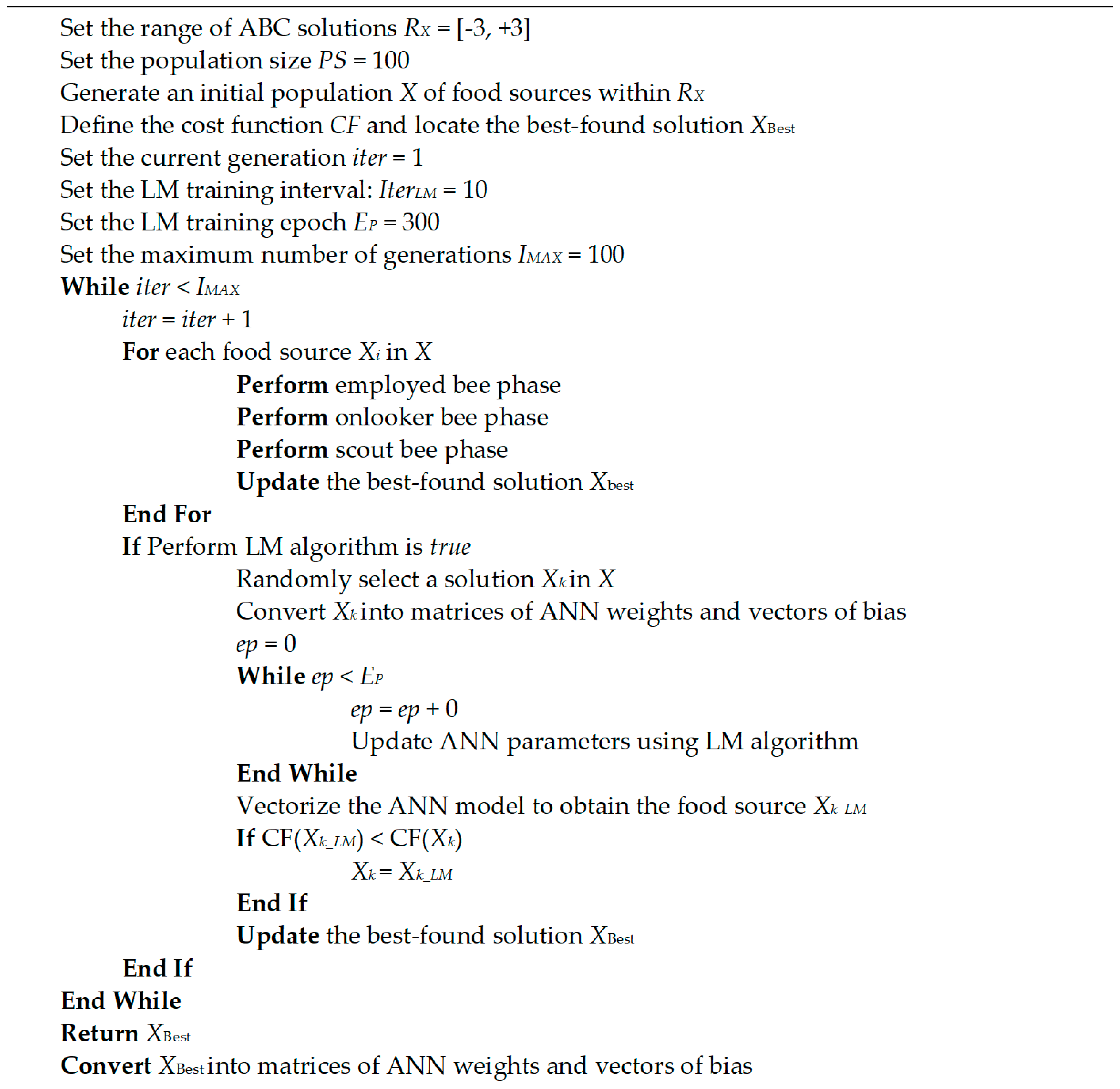
4. Proposed ANN with Hybridization of ABC and LM Algorithms for Compression Coefficient Estimation

This section presents the proposed ANN model trained by a hybrid method of ABC and LM algorithms. This model is trained with the aforementioned experimental dataset and is specifically designed for the task of CC estimation. The proposed model, namely, ABC-LM-ANN, is demonstrated in Figure 5. It is noted that the model relies on the MATLAB Statistics and Machine Learning Toolbox [66] to perform the LM algorithm. In addition, the ABC algorithm and the integrated ABC-LM-ANN model were coded by the authors in MATLAB programming environment.

To construct the ANN model used for CC estimation, it is required to appropriately set the two-weight matrices of W₁ and W₂, as well as the two bias vectors of b₁ and b₂. It is worth reminding that the size of the matrix W₁ is N_R x N_DX, where N_R and N_DX are the numbers of neurons in the hidden layer and the number of input neurons, respectively. Herein, N_DX = 12, which is the number of CC’s conditioning factors. Meanwhile, based on the suggestion of Heaton [67] and several trial-and-error experiments, the value of N_R used in this study is selected to be 10 and the size of W₂ is N_O x N_R where N_O is the number of output neurons. Herein, N_O = 1, which is the targeted output of CC. The size of the two bias vectors of b₁ and b₂ is N_R and 1, respectively. Since it is required that a solution of ABC is presented in the form of a vector, the ANN structure including W₁, W₂, b₁, and b₂ are vectorized and concatenated to formulate a solution or food source. On the basis of the above explanation, the length of a vector representing a solution is N_R x N_DX + N_O x N_R + N_R + 1.

To train the ANN model using the ABC-LM algorithm, the following cost function (CF) is used to minimize the discrepancy between the observed and the predicted output of CC:

$$CF=\frac{MS{E}_{TR}+MS{E}_{VA}}{2}$$

(9)

where MSE_TR and MSE_VA represent the mean squared error (MSE) of the data samples in the training and validating datasets, respectively. Herein, the training set and the validating set occupy 80% and 10% of the whole dataset, respectively. The rest of the original dataset (10%) is reserved for testing purposes.

The MSE is given as follows:

$$MSE=\frac{{{\displaystyle \sum }}_{i=1}^{N_D}{(Y_{A,i}-Y_{P,i})}^2}{N_D}$$

(10)

where Y_A,i and Y_P,i denote the actual and the predicted CC of the ith data instance. N_D is the number of data instances.

The inclusion of the validating data is to safeguard against overfitting during the ABC-LM training process. Overfitting typically occurs when the constructed ANN model can provide a perfect fit to the training data, nevertheless, the model has an inferior fit when predicting CC values for novel soil samples. The inclusion of both training and validating datasets is to force the ABC-LM to seek for a network structure that can deliver good predictive accuracy and guarantee generalization property.

During the model training phase, ABC acts as a global optimizer to guide the population of honeybees to better solutions that represent network structures. Moreover, to accelerate the optimization process, the LM backpropagation algorithm is activated once in ten iterations on a randomly selected solution. With the maximum number of ABC’s iterations set at 100, the LM backpropagation algorithm with the number of training epoch = 300 and the learning rate = 0.01, is activated 10 times to boost the optimization performance. The population size of ABC is chosen to be 100; the lower and upper boundaries of the network parameters, which are the elements of W₁, W₂, b₁, and b₂, are selected to be −3 and 3, respectively. The operational training flow of the ABC-LM algorithm is illustrated in Figure 6.

5. Results and Discussions

As described above earlier, the whole dataset of soil samples includes 441 data points. To construct the ABC-LM-ANN model used for CC prediction, the original dataset is divided into a training set (80%), a validating set (10%), and a testing set (10%). The first two datasets are used in the phase of model construction and the third dataset acts as novel soil samples to verify the predictive performance of the proposed model in real-world applications of CC estimation. It is worth noting that before the model construction and testing phases, the original dataset had been normalized with the use of the Z-score transformation. This data transformation is to prevent the undesired situation in which variables with large magnitude dominate the ones with small magnitude.

To evaluate the performance of the ABC-LM-ANN model, root mean square error (RMSE), the mean absolute percentage error (MAPE), the mean absolute error (MAE), and the coefficient of determination (R²) are employed. The equations used to compute these indices are provided as follows [68]:

$$RMSE=sqrt({\displaystyle \sum }_{t=1}^N\frac{{(Y_{A,i}-Y_{P,i})}^2}{N})$$

(11)

$$MAPE=\frac{100\%}{N}{\displaystyle \sum }_{t=1}^N\frac{\left|Y_{A,i}-Y_{P,i}\right|}{Y_{A,i}}$$

(12)

$$MAE=\frac{1}{N}{\displaystyle \sum }_{t=1}^N\left|Y_{A,i}-Y_{P,i}\right|$$

(13)

$$R^2=\frac{S{S}_{yy}-SSE}{S{S}_{yy}}$$

(14)

where Y_A,i and Y_P,i is the actual and the predicted values of soil CC of the ith data instance. N is the number of data instances in the set of interest.

SS_yy and SEE are calculated as follows:

$${\mathrm{SS}}_{\mathrm{yy}}={\displaystyle \sum }_{\mathrm{i}=1}^{\mathrm{N}}{({\mathrm{Y}}_{\mathrm{A},\mathrm{i}}-{\mathrm{Y}}_{\mathrm{A},\mathrm{m}})}^2$$

(15)

$$SSE={\displaystyle \sum }_{i=1}^N{(Y_{A,i}-Y_{P,i})}^2$$

(16)

where Y_A,m is the mean value of actual soil CC.

The optimization process of the proposed ABC-LM-ANN is illustrated in Figure 7. It can be seen from this figure that the hybridization of ABC and LM can help the searching process to converge into a good solution of ANN structure within 63 iterations. Beyond this point, no better solution of the ANN structure can be found. The ANN optimized by the LM-ANN can attain a promising predictive result with RMSE = 0.009, MAPE = 10.705%, MAE = 0.007, and R² = 0.840. With R² = 0.840 (see Figure 8), the constructed ANN can explain 84% of the variation of the actual CC values. This is a good outcome since the problem of CC estimation, like other problems in the field of geotechnical engineering, is known to be complex. In addition, Figure 9 demonstrates the collected CC values accompanied by the corresponding CC results predicted by the proposed approach and Figure 10 presents the error distribution of the ABC-LM-ANN model in both training and testing phases.

To confirm the performance of the ABC-LM-ANN, its outcome is compared to those of the LM backpropagation artificial neural network (LM-ANN), the ABC trained ANN (ABC-ANN), and the regression tree (RegTree). The two models of LM-ANN and RegTree are implemented in MATLAB environment with the help of the Statistics and Machine Learning Toolbox [66]. To ensure a fair comparison, the hyper-parameters of LM-ANN are selected as follows: the number of neurons in the hidden layer = 10, the learning rate = 0.01, and the maximum number of training epochs = 5000. Moreover, the number of minimum number of leaf node observations is set to be 1 as suggested in [66]. The experimental outcomes are reported in

Table 3. Model result comparison.

Phase	Performance	Prediction Models
		ABC-LM-ANN	LM-ANN	ABC-ANN	RegTree
Training	RMSE	0.009	0.009	0.010	0.005
	MAPE (%)	12.117	11.730	14.674	6.374
	MAE	0.007	0.007	0.008	0.004
	R2	0.860	0.873	0.821	0.955
Testing	RMSE	0.009	0.010	0.010	0.010
	MAPE (%)	10.705	12.400	14.029	12.862
	MAE	0.007	0.008	0.008	0.008
	R2	0.840	0.811	0.792	0.810

. As can be observed from this table, the proposed ABC-LM-ANN has achieved the most desired predictive accuracy with RMSE = 0.009, MAPE = 10.705%, MAE = 0.007, and R² = 0.840. The LM-ANN model is the second-best prediction approach with RMSE = 0.010, MAPE = 12.400%, MAE = 0.008, and R² = 0.811, followed by ABC-ANN (RMSE = 0.010, MAPE = 14.029%, MAE = 0.008, and R² = 0.792) and RegTree (RMSE = 0.010, MAPE = 12.862%, MAE = 0.008, and R² = 0.810).

In the next experiment, to better assess the predictive performance of the proposed ABC-LM-ANN, as well as the other benchmark models, a repetitive random subsampling consisting of 20 training and testing times was performed. In each run, 90% of the data is used for training the CC estimation model and 10% of the data is used as testing cases. The average computational time of the newly developed ABC-LM-ANN is 167.37(s); additionally, the proportions of computational time for global and local searching phases are 97.79% and 2.21%, respectively.

The experimental results obtained from the repeated random subsampling process are reported in

Table 4. The result obtained from the repetitive random subsampling with 20 runs.

Phase	Performance	Prediction Models
		ABC-LM-ANN		LM-ANN		ABC-ANN		RegTree
		Mean	Std	Mean	Std	Mean	Std	Mean	Std
Training	RMSE	0.008	0.000	0.009	0.001	0.011	0.000	0.005	0.000
	MAPE (%)	10.981	0.453	11.585	1.246	15.059	1.053	5.949	0.332
	MAE	0.006	0.000	0.007	0.001	0.008	0.000	0.003	0.000
	R2	0.876	0.009	0.869	0.017	0.811	0.014	0.962	0.004
Testing	RMSE	0.010	0.001	0.010	0.001	0.012	0.001	0.012	0.002
	MAPE (%)	12.586	1.822	13.042	1.520	16.852	3.561	15.015	1.965
	MAE	0.007	0.001	0.008	0.001	0.009	0.001	0.009	0.001
	R2	0.841	0.039	0.817	0.046	0.788	0.057	0.744	0.060

with the mean and the standard deviation (Std) of the outcomes. This second experiment in this study points out that the average testing performance of the ABC-LM-ANN (RMSE = 0.010, MAPE = 12.586%, MAE = 0.007, and R² = 0.841) is better than those of the ANN models trained by LM and ABC, as well as the RegTree model.

Moreover, the two-sample t-test [69] is employed in this section to better demonstrate the statistical significance of the models’ performances differences in terms of R². The R² is selected in this statistical test due to its indication of how well the regression models have fitted the collected dataset. It is noted that the significant level (p-value) of the t-test is 0.05. The outcomes of the two-sample t-test are reported in

Table 5. The t-test results which compare the models’ performances in terms of R²: (a) p-values and (b) model pairwise comparison. Note: “++”, “+”, “--”, and “-” denote a significant win, a win, a significant loss, and a loss, respectively.

(a)
	ABC-LM-ANN	LM-ANN	ABC-ANN	RegTree
ABC-LM-ANN	x	0.11792	0.0018945	1.14E−07
LM-ANN	0.11792	x	0.095532	7.83E−05
ABC-ANN	0.0018945	0.095532	x	0.020189
RegTree	1.14E−07	7.83E−05	0.020189	x
(b)
	ABC-LM-ANN	LM-ANN	ABC-ANN	RegTree
ABC-LM-ANN	x	+	++	++
LM-ANN	-	x	+	++
ABC-ANN	--	-	x	++
RegTree	++	++	++	x

. The results show that the proposed hybrid ABC-LM-ANN has achieved a win over the LM-ANN, as well as two significant wins over ABC-ANN and RegTree. This fact confirms that the proposed ABC-LM-ANN is highly suited for the task of CC estimation.

6. Concluding Remarks

The CC of soil is a crucial geotechnical engineering parameter that is required in the design phase of high-rise housing projects. To avoid the cumbersomeness of the oedometer test, this study proposes a machine learning-based solution for obtaining CC parameter. The machine learning model is established by using ANN with a novel hybrid training method of the ABC and LM algorithms. The ABC metaheuristic acts as a global optimizer which searches for an ANN model that provides the best fit to the collected data. In addition, to accelerate the ABC searching process, the LM backpropagation is performed on a randomly chosen individual of the ABC population. A dataset consisting of 12 predictor variables including sample depth, sand content, loam content clay content, moisture content, wet density, dry density, void ratio, liquid limit, plastic limit, plastic index, and liquid index and 441 soil samples was collected during the construction phase of a large-scale housing project in Vietnam. This dataset is, then, employed to train and verify the prediction performance of the newly constructed ABC-LM-ANN model. Experimental results confirm that ABC-LM-ANN can deliver the prediction result of CC which is superior to those of other benchmark approaches. Therefore, the newly established model can be a promising alternative to assist the decision-making process in the design phase of high-rise housing projects. Future research works could consider new robust optimization algorithms to improve the prediction performance of CC.

As can be confirmed by the reported experimental results, one significant advantage of the hybrid ABC-LM-ANN model is that it combines the two powerful methods of training neural network regression to achieve a good predictive performance of CC parameter estimation. Therefore, the model is capable of delivering reliable estimations of this property of soil to quickly assist the engineering decision-making process. However, one difficulty of using the model is that there are a set of model hyper-parameters (e.g., the population size of the ABC, the maximum number of epochs used in the LM training operator, and the number of neurons in the hidden layer) needed to be tuned empirically. Furthermore, the current model does not integrate with the feature selection method, and therefore employing metaheuristic-based feature evaluation could be a potential extension of this study.

References

1. Ahmed, S.I.; Siddiqua, S. Compressibility behavior of soils: A statistical approach. Geotech. Geologi. Eng. 2016, 34, 2063–2070. [Google Scholar] [CrossRef]
2. Chummar, A.V. Excessive settlement in buildings. In Proceedings of the First International Conference on Case Histories in Geotechnical Engineering, St. Louis, MO, USA, 6–11 May 1984. [Google Scholar]
3. Srivastava, A.; Goyal, C.R.; Jain, A. Review of causes of foundation failures and their possible preventive and remedial measures. In Proceedings of the 4th KKU—International Engineering Conference, (KKU-IENC2012), Khon Kaen, Thailand, 10–11 May 2012. [Google Scholar]
4. Anastasopoulos, I. Structural damage of a 5-storey building: Differential settlement due to construction of an adjacent building or because of construction defects? In Proceedings of the Seventh International Conference on Case Histories in Geotechnical Engineering, Chicago, IL, USA, 1–4 May 2013. [Google Scholar]
5. Charles, R.D. Case history of two building experience large post construction settlements—Wilmington, delaware. In Proceedings of the Fourth International Conference on Case Histories in Geotechnical Engineering, St. Louis, MO, USA, 9–12 March 1998. [Google Scholar]
6. Zhu, M.; Gary, T.B.; Bachus, R.C. Assessment of a building settlement and the litigation process—A case study. In Proceedings of the Sixth Congress on Forensic Engineering, San Francisco, CA, USA, 31 October –3 November 2012. [Google Scholar]
7. Kim, Y.J.; Gajan, S.; Saafi, M. Settlement rehabilitation of a 35-year-old building: Case study integrated with analysis and implementation. Pract. Periodi. Struct. Des. Constr. 2011, 16, 215–222. [Google Scholar] [CrossRef]
8. Mohammadzadeh, D.; Bolouri, B.J.; Alavi, A.H. An evolutionary computational approach for formulation of compression index of fine-grained soils. Eng. Appl. Artif. Intell. 2014, 33, 58–68. [Google Scholar] [CrossRef]
9. Gulhati, S.K.; Datta, M. Geotechnical Engineering; Tata Mc Graw Hill Publishing Company Limited: New York, NY, USA, 2005. [Google Scholar]
10. Mohammadzadeh, S.D.; Bolouri, B.J.; Vafaee, J.Y.S.H.; Alavi, A.H. Deriving an intelligent model for soil compression index utilizing multi-gene genetic programming. Environ. Earth Sci. 2016, 75, 262. [Google Scholar] [CrossRef]
11. Tiwari, B.; Ajmera, B. New correlation equations for compression index of remolded clays. J. Geotech. Geoenviron. Eng. 2012, 138, 757–762. [Google Scholar] [CrossRef]
12. Mohammadzadeh, S.; Kazemi, S.-F.; Mosavi, A.; Nasseralshariati, E.; Tah, J.H. Prediction of compression index of fine-grained soils using a gene expression programming model. Infrastructures 2019, 4, 26. [Google Scholar] [CrossRef]
13. Terzaghi, K.; Peck, R.B.; Mesri, G. Soil Mechanics in Engineering Practice; John Wiley & Sons, Inc: Hoboken, NJ, USA, 1996. [Google Scholar]
14. Polidori, E. On the intrinsic compressibility of common clayey soils. Eur. J. Environ. Civil Eng. 2015, 19, 27–47. [Google Scholar] [CrossRef]
15. Puri, N.; Prasad, H.D.; Jain, A. Prediction of geotechnical parameters using machine learning techniques. Proced. Comput. Sci. 2018, 125, 509–517. [Google Scholar] [CrossRef]
16. Moayed, R.Z.; Kordnaeij, A.; Mola-Abasi, H. Compressibility indices of saturated clays by group method of data handling and genetic algorithms. Neural Comput. Appl. 2017, 28, 551–564. [Google Scholar] [CrossRef]
17. Kurnaz, T.F.; Dagdeviren, U.; Yildiz, M.; Ozkan, O. Prediction of compressibility parameters of the soils using artificial neural network. SpringerPlus 2016, 5, 1801. [Google Scholar] [CrossRef]
18. Gupta, S.C.; Allmaras, R.R. Models to Assess the Susceptibility of Soils to Excessive Compaction; Springer: New York, NY, USA, 1987; pp. 65–100. [Google Scholar]
19. Kirts, S.; Panagopoulos, O.P.; Xanthopoulos, P.; Nam, B.H. Soil-compressibility prediction models using machine learning. J. Comput. Civ. Eng. 2018, 32, 04017067. [Google Scholar] [CrossRef]
20. McNabb, D.H.; Boersma, L. Nonlinear model for compressibility of partly saturated soils. Soil Sci. Soc. Am. J. 1996, 60, 333–341. [Google Scholar] [CrossRef]
21. Pham, B.T.; Son, L.H.; Hoang, T.-A.; Nguyen, D.-M.; Tien Bui, D. Prediction of shear strength of soft soil using machine learning methods. Catena 2018, 166, 181–191. [Google Scholar] [CrossRef]
22. Tien Bui, D.; Hoang, N.-D.; Nhu, V.-H. A swarm intelligence-based machine learning approach for predicting soil shear strength for road construction: A case study at trung luong national expressway project (vietnam). Eng. Comput. 2018, 35, 955–965. [Google Scholar] [CrossRef]
23. Hashemi Jokar, M.; Mirasi, S. Using adaptive neuro-fuzzy inference system for modeling unsaturated soils shear strength. Soft Comput. 2017, 22, 4493–4510. [Google Scholar] [CrossRef]
24. Mohammad Emami, N.; Rasool Amiri, K.; Mohammad Khodaiy, A.; Mahdi Shahbazi, R. Metaheuristic optimization approaches to predict shear-wave velocity from conventional well logs in sandstone and carbonate case studies. J. Geophys. Eng. 2018, 15, 1071. [Google Scholar]
25. Chou, J.-S.; Yang, K.-H.; Lin, J.-Y. Peak shear strength of discrete fiber-reinforced soils computed by machine learning and metaensemble methods. J. Comput. Civ. Eng. 2016, 30, 04016036. [Google Scholar] [CrossRef]
26. Tang, X.W.; Bai, X.; Hu, J.L.; Qiu, J.N. Assessment of liquefaction-induced hazards using bayesian networks based on standard penetration test data. Nat. Hazards Earth Syst. Sci. 2018, 18, 1451–1468. [Google Scholar] [CrossRef]
27. Hoang, N.-D.; Bui, D.T. Predicting earthquake-induced soil liquefaction based on a hybridization of kernel fisher discriminant analysis and a least squares support vector machine: A multi-dataset study. Bull. Eng. Geol. Environ. 2018, 77, 191–204. [Google Scholar] [CrossRef]
28. Prayogo, D.; Susanto, Y.T.T. Optimizing the prediction accuracy of friction capacity of driven piles in cohesive soil using a novel self-tuning least squares support vector machine. Adv. Civ. Eng. 2018, 2018, 9. [Google Scholar] [CrossRef]
29. Moayedi, H.; Hayati, S. Applicability of a cpt-based neural network solution in predicting load-settlement responses of bored pile. Int. J. Geomech. 2018, 18, 06018009. [Google Scholar] [CrossRef]
30. Tekin, E.; Akbas, S.O. Predicting groutability of granular soils using adaptive neuro-fuzzy inference system. Neural Comput. Appl. 2017, 31, 1091–1101. [Google Scholar] [CrossRef]
31. Hoang, N.-D.; Tien Bui, D.; Liao, K.-W. Groutability estimation of grouting processes with cement grouts using differential flower pollination optimized support vector machine. Appl. Soft Comput. 2016, 45, 173–186. [Google Scholar] [CrossRef]
32. Bishop, C.M. Information Science and Statistics. In Pattern Recognition and Machine Learning; Jordan, M.I., Robert, N., Bernhard, S., Eds.; Springer: Berlin/Heidelberg, Germany, 2011. [Google Scholar]
33. Bishop, C.M. Neural Networks for Pattern Recognition; Oxford university press: Oxford, UK, 1995. [Google Scholar]
34. Shahin, M.A. State-of-the-art review of some artificial intelligence applications in pile foundations. Geosci. Front. 2016, 7, 33–44. [Google Scholar] [CrossRef]
35. Park, H.I.; Lee, S.R. Evaluation of the compression index of soils using an artificial neural network. Comput. Geotech. 2011, 38, 472–481. [Google Scholar] [CrossRef]
36. Hoang, N.-D.; Chen, C.-T.; Liao, K.-W. Prediction of chloride diffusion in cement mortar using multi-gene genetic programming and multivariate adaptive regression splines. Measurement 2017, 112, 141–149. [Google Scholar] [CrossRef]
37. Tran, T.-H.; Hoang, N.-D. Predicting colonization growth of algae on mortar surface with artificial neural network. J. Comput. Civ. Eng. 2016, 30, 04016030. [Google Scholar] [CrossRef]
38. Montavon, G.; Orr, G.; Müller, K.-R. Neural Networks: Tricks of the Trade; Springer: Berlin/Heidelberg, Germany, 2012. [Google Scholar]
39. Pham, B.T.; Tien Bui, D.; Prakash, I.; Dholakia, M.B. Hybrid integration of multilayer perceptron neural networks and machine learning ensembles for landslide susceptibility assessment at himalayan area (india) using gis. Catena 2017, 149 Pt 1, 52–63. [Google Scholar] [CrossRef]
40. Georgiou, P.; Plati, C.; Loizos, A. Soft computing models to predict pavement roughness: A comparative study. Adv. Civ. Eng. 2018, 2018, 8. [Google Scholar] [CrossRef]
41. Ojha, V.K.; Abraham, A.; Snášel, V. Metaheuristic design of feedforward neural networks: A review of two decades of research. Eng. Appl. Artif. Intell. 2017, 60, 97–116. [Google Scholar] [CrossRef]
42. Göçken, M.; Özçalıcı, M.; Boru, A.; Dosdoğru, A.T. Integrating metaheuristics and artificial neural networks for improved stock price prediction. Expert Syst. Appl. 2016, 44, 320–331. [Google Scholar] [CrossRef]
43. Hacibeyoglu, M.; Ibrahim, M.H. A novel multimean particle swarm optimization algorithm for nonlinear continuous optimization: Application to feed-forward neural network training. Sci. Program. 2018, 2018, 9. [Google Scholar] [CrossRef]
44. Rere, L.M.R.; Fanany, M.I.; Arymurthy, A.M. Metaheuristic algorithms for convolution neural network. Comput. Intell. Neurosci. 2016, 2016, 13. [Google Scholar] [CrossRef] [Green Version]
45. Taheri, K.; Hasanipanah, M.; Golzar, S.B.; Majid, M.Z.A. A hybrid artificial bee colony algorithm-artificial neural network for forecasting the blast-produced ground vibration. Eng. Comput. 2017, 33, 689–700. [Google Scholar] [CrossRef]
46. Ghasemiyeh, R.; Moghdani, R.; Sana, S.S. A hybrid artificial neural network with metaheuristic algorithms for predicting stock price. Cybern. Syst. 2017, 48, 365–392. [Google Scholar] [CrossRef]
47. Tien Bui, D.; Le, H.V.; Hoang, N.-D. Gis-based spatial prediction of tropical forest fire danger using a new hybrid machine learning method. Ecol. Inform. 2018, 48, 104–116. [Google Scholar] [CrossRef]
48. Kose, U. An ant-lion optimizer-trained artificial neural network system for chaotic electroencephalogram (eeg) prediction. Appl. Sci. 2018, 8, 1613. [Google Scholar] [CrossRef] [Green Version]
49. Piotrowski, A.P. Differential evolution algorithms applied to neural network training suffer from stagnation. Appl. Soft Comput. 2014, 21, 382–406. [Google Scholar] [CrossRef]
50. Karaboga, D.; Basturk, B. A powerful and efficient algorithm for numerical function optimization: Artificial bee colony (abc) algorithm. J. Glob. Optim. 2007, 39, 459–471. [Google Scholar] [CrossRef]
51. Hagan, M.T.; Menhaj, M.B. Training feedforward networks with the marquardt algorithm. IEEE Trans. Neural Netw. 1994, 5, 989–993. [Google Scholar] [CrossRef]
52. Karaboga, D.; Gorkemli, B.; Ozturk, C.; Karaboga, N. A comprehensive survey: Artificial bee colony (abc) algorithm and applications. Artif. Intell. Rev. 2014, 42, 21–57. [Google Scholar] [CrossRef]
53. Tien Bui, D.; Tuan, T.A.; Hoang, N.-D.; Thanh, N.Q.; Nguyen, D.B.; Van Liem, N.; Pradhan, B. Spatial prediction of rainfall-induced landslides for the lao cai area (vietnam) using a hybrid intelligent approach of least squares support vector machines inference model and artificial bee colony optimization. Landslides 2017, 14, 447–458. [Google Scholar] [CrossRef]
54. Ghaleini, E.N.; Koopialipoor, M.; Momenzadeh, M.; Sarafraz, M.E.; Mohamad, E.T.; Gordan, B. A combination of artificial bee colony and neural network for approximating the safety factor of retaining walls. Eng. Comput. 2018, 35, 647–658. [Google Scholar] [CrossRef]
55. Baldo, N.; Manthos, E.; Pasetto, M. Analysis of the mechanical behaviour of asphalt concretes using artificial neural networks. Adv. Civ. Eng. 2018, 2018, 17. [Google Scholar] [CrossRef] [Green Version]
56. Tien Bui, D.; Nhu, V.-H.; Hoang, N.-D. Prediction of soil compression coefficient for urban housing project using novel integration machine learning approach of swarm intelligence and multi-layer perceptron neural network. Adv. Eng. Inform. 2018, 38, 593–604. [Google Scholar] [CrossRef]
57. Moayedi, H.; Mosallanezhad, M.; Rashid, A.S.A.; Jusoh, W.A.W.; Muazu, M.A. A systematic review and meta-analysis of artificial neural network application in geotechnical engineering: Theory and applications. Neural Comput. Appl. 2018, 1–24. [Google Scholar] [CrossRef]
58. Sulewska, M.J. Applying artificial neural networks for analysis of geotechnical problems. Comput. Assist. Method. Eng. Sci. 2017, 18, 231–241. [Google Scholar]
59. Tien Bui, D.; Hoang, N.-D.; Martínez-Álvarez, F.; Ngo, P.-T.T.; Hoa, P.V.; Pham, T.D.; Samui, P.; Costache, R. A novel deep learning neural network approach for predicting flash flood susceptibility: A case study at a high frequency tropical storm area. Sci. Total Environ. 2019, 2019, 134413. [Google Scholar] [CrossRef]
60. Ngo, P.T.; Hoang, N.D.; Pradhan, B.; Nguyen, Q.K.; Tran, X.T.; Nguyen, Q.M.; Nguyen, V.N.; Samui, P.; Tien Bui, D. A novel hybrid swarm optimized multilayer neural network for spatial prediction of flash floods in tropical areas using Sentinel-1 SAR imagery and geospatial data. Sensors 2018, 18, 3704. [Google Scholar] [CrossRef] [Green Version]
61. Zhongya, Z.; Xiaoguang, J. Prediction of peak velocity of blasting vibration based on artificial neural network optimized by dimensionality reduction of fa-miv. Math. Probl. Eng. 2018, 2018, 12. [Google Scholar] [CrossRef]
62. Gordan, B.; Koopialipoor, M.; Clementking, A.; Tootoonchi, H.; Tonnizam Mohamad, E. Estimating and optimizing safety factors of retaining wall through neural network and bee colony techniques. Eng. Comput. 2018, 35, 945–954. [Google Scholar] [CrossRef]
63. Lera, G.; Pinzolas, M. Neighborhood based Levenberg-Marquardt algorithm for neural network training. IEEE Trans. Neural Netw. 2002, 13, 1200–1203. [Google Scholar] [CrossRef]
64. Pham, B.T.; Nguyen, M.D.; Bui, K.T.T.; Prakash, I.; Chapi, K.; Bui, D.T. A novel artificial intelligence approach based on Multi-layer Perceptron Neural Network and Biogeography-based Optimization for predicting coefficient of consolidation of soil. Catena 2019, 173, 302–311. [Google Scholar] [CrossRef]
65. Clayton, C.R. The Standard Penetration Test (spt): Methods and Use; Construction Industry Research and Information Association: London, UK, 1995. [Google Scholar]
66. Matwork. Statistics and Machine Learning Toolbox User’s Guide. Matwork Inc.; Available online: https://www.mathworks.com/help/pdf_doc/stats/stats.pdf (accessed on 28 April 2018).
67. Heaton, J. Volume 3 Deep Learning and Neural Networks. In Artificial Intelligence for Humans; Heaton Research: St. Louis, MO, USA, 2015. [Google Scholar]
68. Nhu, V.-H.; Samui, P.; Kumar, D.; Singh, A.; Hoang, N.-D.; Bui, D.T. Advanced soft computing techniques for predicting soil compression coefficient in engineering project: A comparative study. Eng. Comput. 2019, 1–12. [Google Scholar] [CrossRef]
69. Snedecor, G.W.; Cochran, W.G. Statistical Methods, 8th ed.; Iowa State University Press: Iowa City, Iowa, 1989. [Google Scholar]
Figure 1. A typical structure of the neural network.
Applsci 09 04912 g001
Figure 2. Location of the study area.
Applsci 09 04912 g002
Figure 3. Histograms of compression coefficient’s influencing variables.
Applsci 09 04912 g003
Figure 4. Histograms of the compression coefficient as the response variable.
Applsci 09 04912 g004
Figure 5. The proposed artificial bee colony Levenberg–Marquardt artificial neural network (ABC-LM-ANN) for compression coefficient (CC) estimation.
Applsci 09 04912 g005
Figure 6. The training flow of the ABC-LM algorithm.
Applsci 09 04912 g006
Figure 7. The optimization process of the LM-ANN approach.
Applsci 09 04912 g007
Figure 8. The performance of the proposed ABC-LM-ANN model used for predicting CC.
Applsci 09 04912 g008
Figure 9. The actual CC vs. the value of CC predicted by the proposed ABC-LM-ANN model.
Applsci 09 04912 g009
Figure 10. The error distribution of ABC-LM-ANN.
Applsci 09 04912 g010