Abstract
We show that by treating the weak probe field as a perturbation to the strong coupling fields in the atomic system and using the perturbative method in a master equation, the features of linear response of phenomena of electromagnetically induced transparency (EIT) can be uniformly demonstrated, regardless of the details of atomic energy level configuration. We compare our estimation with both typical and atypical EIT-observed configurations and find that our model indeed provides a description of the sharp transmission window in central area of typical EIT curve. It can also be inferred hereby that for various systems other than atomic gas, as long as the description of the system’s dynamics comes down to the simplified form of master equation, the corresponding EIT analogs and EIT-like phenomena can also be explained in this way.
1. Introduction
First demonstrated on -type atomic configuration [1], electromagnetically induced transparency (EIT) is a phenomenon observed in multilevel atomic systems [2,3,4,5,6,7,8,9,10] where a weak probe field, in the presence of strong coupling fields, experiences suppression of resonant absorption and sees a steep dispersion. Making an initially opaque medium transparent to a probe laser beam, EIT has been explained in terms of the destructive quantum interference effect between different excitation pathways [11], or a dark superposition state [12,13,14] in the multistate system. Due to the fact that EIT provides the possibility of wide applications in light velocity control [15,16,17], quantum information [18,19,20] and nonlinear optics [21], there have been many works carried out on this subject. Traditionally in the study of EIT, the analytical expression of the atomic medium optical susceptibility is calculated based on the specific atomic configuration [2,3,4,5,6,7,8,9,10], although the general features of the EIT phenomena are basically the same regardless of the configuration details. On the other hand, EIT-like phenomena can be found in many different systems, such as interacting classical harmonic oscillators [22], coupled microcavities [23,24,25], waveguide resonators [26,27,28,29,30], and so on. Noticing the wide existence of EIT and EIT-like phenomena, we feel this could be a hint for us to find a more general viewpoint for the description of EIT.
In this paper, we present a perturbative view from master equation for EIT, by treating the applied fields—strong coupling fields as first order and weak probe field as second order perturbation to the atomic system, and by using the perturbative approach of master equation, we find that the analytical expression of the probe response susceptibility could explain the shape of the sharp transmission window of EIT, without involving the details of the atomic energy level configuration. The perturbative approach of density matrix we use here is some kind of standard treatment in many fields, say, nonlinear optics [31], and we adopt it here to bring on the new view of demonstration of EIT, which to the best of our knowledge, has not been done before. We are hoping this work would help deepening our understanding of the wide existence of EIT analogs and EIT-related phenomena.
2. The Model
Imagine we have an initial atomic system, and by applying the strong coupling fields to the system, the state population is modified. We then add the weak probe field, and the state population will be slightly modified again. Thus we see, the difference made by the adding-on of the probe field is the optical response of the atomic system to the probe field. Correspondingly in calculation, we apply the strong coupling fields as perturbation to the Hamiltonian of the original atomic system in master equation, and do the first order perturbation calculation. Following that, we do the second order perturbation calculation, where we throw in the weak probe field, the effect of which will be used to deduce the expression of the atomic system’s linear optical susceptibility. We point out that in the treatment of the perturbation, when including the strong coupling fields and weak probe field as a whole, the different orders of nonlinear susceptibility can all be looked into; however, the features of EIT we study only involve the one particular term corresponding to the linear probe susceptibility.
As described above, treating all applied fields as a perturbation to the atomic system, we take the strong coupling fields as the first order perturbation and the weak probe field as the second order; the Hamiltonian of the system can be written as
where is the parameter characterizing the strength of the perturbation, ranging between 0 and 1. is the Hamiltonian of the free atomic system, is the interaction energy corresponding to the strong coupling fields, and is the interaction energy corresponding to the weak probe field.
We then seek a solution of the density matrix element in the power series of up to second order
As discussed before, we expect the lowest order contribution of to be related to the atomic media’s optical response to the probe field.
Starting with the general form of master equation
where is the decay rate of , we plug in the expression of from (1), noting that , we then have
In the above we define as the resonant transition frequency between energy levels and of the atom. Then, when only adding in the strong coupling fields in interaction, from Equation (4) we have
On the other hand, in the second round we turn on the weak probe field and only look at the modification it brings to , because a modification of probe field to , which is
means the effect of the weak probe field without presence of strong coupling fields, and this is obviously not the case of EIT we are considering.
The modified at presence of weak probe field is
the difference brought up by the insertion of weak probe field is
which is the order correction to . This corresponds to the susceptibility induced by weak probe field in the presence of strong coupling fields. To figure out the expression of , we first calculate the first order correction .
For the strong coupling fields, we suppose is in the form
with
being the field at frequency coupling atomic states and with relevant dipole moment . Under the assumption that the unperturbed density matrix element is given by for , we have
and we therefore can write down
We then assume the weak probe field is applied between the atomic states and , so that
where is the amplitude of the probe field, is the relevant dipole moment between the atom’s energy levels and , and is the frequency of the probe field. Then
Since the above expression is analogous to the one in Equation (12), we can easily deduce from analogy between Equations (5) and (6) and comparison to Equation (13) that
and this is the in Equation (9) we are looking for.
From the above results, we can get the expression of probe susceptibility. Normally, the expectation value of the probe field-related induced dipole moment should be decomposed into sum of different frequency components as . Since in our case there is only one frequency existing in the probe field, we have
On the other hand the probe susceptibility can be defined in equation
where and is the number density of atoms. It is then straightforward to see that can be expressed as
Please note that the superscript 2 of means the probe field effect only comes up in the second order perturbation of the system instead of first order, but physically it still indicates the highest order contribution of the probe field, which is the linear probe susceptibility.
For isotropic atomic media, we can rewrite Equation (19) as the scalar quantity
where we define the probe field frequency detuning as , then when we draw a plot of the real and imaginary parts of as the function of , assuming , we find that the shape of just coincide with the dip in the absorption of EIT, and coincide with the sharp dispersion window in the refraction of EIT, within the central area . However, when gets larger, Equation (20) is not suitable to give the description of EIT profile.
3. Examples: Comparison of Our Model with a Set of Multilevel Structures
To demonstrate our results from the previous section, we use the example of multilevel atomic structure given by [6], the schematic diagram of which is drawn in Figure 1, to compare the EIT curves of the most typical special cases of this multilevel structure with the result of Equation (20).
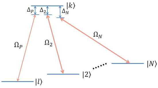
Figure 1.
Schematic diagram of the level atomic system. The upper level state is labeled , and the lower level states are labeled , , . The energy levels are coupled by N coherent laser fields on each upper-lower pair. The corresponding Rabi frequencies and field detunings of the coupling fields are , , and , , .
The structure of the multilevel system is as follows: There are 1 upper energy level state and N lower energy level states, coupled by N coherent laser fields between each upper-lower level pair. For convenience of comparison we label the upper energy state as , the first lower energy state as , and the rest of the lower energy states as to accordingly. The Rabi frequencies of each coupling field between , , are , , , and the corresponding laser field detunings are , , .
As shown in [6], the linear probe susceptibility of the above multilevel structure can be expressed as
which is obtained under the weak probe field limit, and where we have assumed . In this multilevel structure all the () are set to be zero. For the case study, we now look at the structures of and . When , the multilevel system is the type configuration, and when , the system turns into the tripod type configuration. As for the parameter setting, we take the value of as unit and choose , as the typical value setting, together with the assumption , (on-resonance strong field coupling). Then dropping the constant part in both Equation (20) and Equation (21) and adding a minus sign to Equation (20), the imaginary and real part as a function of , in cases of type, tripod type, and result of Equation (20), are plotted in Figure 1a,b.
As can be seen from Figure 2a,b, when is small enough, Equation (20) gives the very close description of EIT curve to that given by type and tripod type from Equation (21). However, when gets larger, there is obvious deviation of our estimation from the curves of and tripod configuration. This can be easily understood. Under large detuning the weak probe field is not effectively coupled to the system, so Equation (20), which is obtained from treating the probe field as perturbation to the system is not suitable for this area. Alternatively from the point of view of atomic physics, Equation (20) describes optical response of the stable atomic media, which means we measure the optical response some time after the atom-field interaction. In this case the only coupling field frequency that need to be considered is the on-resonance one, so what survives through Equation (20) is the probe field satisfying .
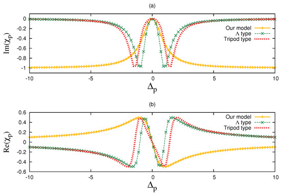
Figure 2.
The comparison of our estimation from Equation (20) and two special cases from Equation (21) for linear probe susceptibility as function of probe field detuning . The type configuration corresponds to the case in Equation (21), and the tripod type corresponds to the case in Equation (21). The parameter settings are , , , in unit of . The results are separately plotted as: (a) The absorption spectra (imaginary part of ) as function of . Here besides the minus sign, there is a offset of unit 1 in y direction in the plot of our model. (b) The dispersion spectra (real part of ) as function of .
We can also look at the case of Equation (21), which we call five-leg type, and the ladder type (or type), which although is different from the type, still shares the same expression of probe susceptibility under the assumption of on-resonance strong field coupling () [3]. The difference between the ladder type and type in parameter setting is that for ladder type. We set , , , , and all the other parameters the same as in Figure 2 and get the results of comparison in Figure 3. As can be seen from the plot, the probe susceptibility curves of five-leg and ladder configurations do not coincide with our model now, because they are not typical EIT configurations any more. Equation (21) shows that a five-leg configuration under our parameter setting is equivalent to a type configuration with doubled Rabi frequency. Also, for the ladder type configuration, the existence of nonzero decay rate brings atypical EIT observation.
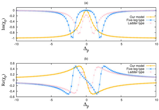
Figure 3.
The comparison of our estimation from Equation (20) with five-leg type and ladder type in probe susceptibility as function of probe field detuning . The five-leg type is the case in Equation (21). The ladder type shares the same expression with type from Equation (21), under assumption that the strong field () coupling is on-resonance. The parameter settings are as follows: , in unit of . Also, for ladder type, () for five-leg type. The results are separately plotted as: (a) The absorption spectra (imaginary part of ) as function of . Here besides the minus sign, there is a offset of unit 1 in y direction in the plot of our model. (b) The dispersion spectra (real part of ) as function of .
When deviates from zero, the existence of a weak probe field can be ignored, and the measurement of probe susceptibility between energy levels and is equivalently performed on the system with only all the strong coupling fields existing. The entire EIT curve can therefore be looked on as the combination of two parts: the profile determined by the presence of strong coupling fields, and the steep change imposed on the central area of by the weak probe field. The latter has been described by Equation (20), then how do we figure out the shape of the former? In addition, why there is a minus sign needed when Equation (20) is used to describe the central area of EIT phenomena? We may not be able to answer these questions in the most general cases; however, when the polarization of all the applied fields are of the same direction, these two questions can be answered together.
Here is the imaginary operation that we perform. Suppose all the applied fields are of the same polarization direction , and all the strong coupling fields from Equation (10) are of the similar magnitude , i.e., , then we know there is also for the weak probe field. We now apply a set of adjusting electric fields , where as defined in Equation (11), coupled to the corresponding energy levels and , can also be approximately written as . We then have
For the probe field coupling energy levels and , we apply
which is in reverse direction of , but with a much larger amplitude . Comparing Equation (22) and Equation (23), we see that from the outside point of view, the entire atomic structure involved with applied fields (both strong coupling fields and weak probe field) is uniformly covered by a “coat” of reverse electric field of magnitude ∼. We now assume the induced energy shift of all the involved energy levels are also of similar magnitude and are small enough to be ignored, then it is safe to say that the atomic structure is not altered by the reverse electric field “coat”, neither is the intrinsic feature of the optical response of the atomic media. The change brought on by the reverse “coat” is that it cancels out all the strong coupling fields, while replacing the initial weak probe field with a strong and reverse one. We are now in the simple case of Lorentz oscillator model, which gives the profile shape of EIT curve outside the central area. Due to the reversed direction of the “new” strong probe field compared to the “old” weak one, there must be a minus sign emerging in front of Equation (20) in adding up the on-resonance dip and the off-resonance profile, as long as the labels of the involved energy level states are unchanged. Thus, the shape of the entire EIT curve has been explained.
4. Conclusions
In summary, we have used the perturbative method in a master equation, by treating the applied fields as first and second order perturbation to the atomic system, to get the analytical expression of probe susceptibility regardless of the details of atomic configuration, which demonstrates the features of EIT phenomena. Our work can also be used to explain the widely existing EIT analogs and EIT-like phenomena, as long as the description of the system’s dynamics comes down to the simplified form of master equation.
Funding
This research was funded by the NSFC No. 11847244, 11534002, 11447609.
Conflicts of Interest
The author declares no conflict of interest.
Abbreviations
The following abbreviation are used in this manuscript:
| EIT | electromagnatically induced transparency |
References
- Boller, K.-J.; Glu, A.I.; Harris, S.E. Observation of electromagnetically induced transparency. Phys. Rev. Lett. 1991, 66, 2593–2596. [Google Scholar] [CrossRef] [PubMed]
- Harris, S.E.; Field, J.E.; Kasapi, A. Dispersive properties of electromagnetically induced transparency. Phys. Rev. A 1992, 46, R29–R32. [Google Scholar] [CrossRef] [PubMed]
- Gea-Banacloche, J.; Li, Y.-Q.; Jin, S.-Z.; Xiao, M. Electromagnetically induced transparency in ladder-type inhomogeneously broadened media: Theory and experiment. Phys. Rev. A 1995, 51, 576–584. [Google Scholar] [CrossRef] [PubMed]
- Li, Y.-Q.; Xiao, M. Electromagnetically induced transparency in a three-level Λ-type system in rubidium atoms. Phys. Rev. A 1995, 51, R2703–R2706. [Google Scholar] [CrossRef] [PubMed]
- Fulton, D.J.; Shepherd, S.; Moseley, R.R.; Sinclair, B.D.; Dunn, M.H. Continuous-wave electromagnetically induced transparency: A comparison of V, Λ, and cascade systems. Phys. Rev. A 1995, 52, 2302–2311. [Google Scholar] [CrossRef] [PubMed]
- Paspalakis, E.; Knight, P.L. Electromagnetically induced transparency and controlled group velocity in a multilevel system. Phys. Rev. A 2002, 66, 015802. [Google Scholar] [CrossRef]
- Wu, Y.; Yang, X. Electromagnetically induced transparency in V-, Λ-, and cascade-type schemes beyond steady-state analysis. Phys. Rev. A 2005, 71, 053806. [Google Scholar] [CrossRef]
- Petrosyan, D.; Otterbach, J.; Fleischhauer, M. Electromagnetically Induced Transparency with Rydberg Atoms. Phys. Rev. Lett. 2011, 107, 213601. [Google Scholar] [CrossRef]
- Mirza, A.B.; Singh, S. Wave-vector mismatch effects in electromagnetically induced transparency in Y-type systems. Phys. Rev. A 2012, 85, 053837. [Google Scholar] [CrossRef]
- Yan, D.; Liu, Y.-M.; Bao, Q.-Q.; Fu, C.-B.; Wu, J.-H. Electromagnetically induced transparency in an inverted-Y system of interacting cold atoms. Phys. Rev. A 2012, 86, 023828. [Google Scholar] [CrossRef]
- Harris, S.E. Lasers without inversion: Interference of lifetime-broadened resonances. Phys. Rev. Lett. 1989, 62, 1033–1036. [Google Scholar] [CrossRef] [PubMed]
- Fleischhauer, M.; Lukin, M.D. Dark-State Polaritons in Electromagnetically Induced Transparency. Phys. Rev. Lett. 2000, 84, 5094–5097. [Google Scholar] [CrossRef] [PubMed]
- Wong, V.; Boyd, R.W.; Stroud, C.R., Jr.; Bennink, R.S.; Aronstein, D.L.; Park, Q.H. Absorptionless self-phase-modulation via dark-state electromagnetically induced transparency. Phys. Rev. A 2001, 65, 013810. [Google Scholar] [CrossRef]
- Qi, J.; Lyyra, A.M. Electromagnetically induced transparency and dark fluorescence in a cascade three-level diatomic lithium system. Phys. Rev. A 2006, 73, 043810. [Google Scholar] [CrossRef]
- Hau, L.V.; Harris, S.E.; Dutton, Z.; Behroozi, C.H. Light speed reduction to 17 metres per second in an ultracold atomic gas. Nature 1999, 397, 594–598. [Google Scholar] [CrossRef]
- Budker, D.; Kimball, D.F.; Rochester, S.M.; Yashchuk, V.V. Nonlinear Magneto-optics and Reduced Group Velocity of Light in Atomic Vapor with Slow Ground State Relaxation. Phys. Rev. Lett. 1999, 83, 1767–1770. [Google Scholar] [CrossRef]
- Phillips, D.F.; Fleischhauer, A.; Mair, A.; Walsworth, R.L.; Lukin, M.D. Storage of Light in Atomic Vapor. Phys. Rev. Lett. 2001, 86, 783–786. [Google Scholar] [CrossRef]
- Lvovsky, A.I.; Sanders, B.C.; Tittel, W. Optical quantum memory. Nat. Photonics 2009, 3, 706–714. [Google Scholar] [CrossRef]
- Souza, J.A.; Figueroa, E.; Chibani, H.; Villas-Boas, C.J.; Rempe, G. Coherent Control of Quantum Fluctuations Using Cavity Electromagnetically Induced Transparency. Phys. Rev. Lett. 2013, 111, 113602. [Google Scholar] [CrossRef]
- Shomroni, I.; Rosenblum, S.; Lovsky, Y.; Bechler, O.; Guendelman, G.; Dayan, B. All-optical routing of single photons by a one-atom switchcontrolled by a single photon. Science 2014, 345, 903–906. [Google Scholar] [CrossRef]
- Harris, S.E.; Hau, L.V. Nonlinear Optics at Low Light Levels. Phys. Rev. Lett. 1999, 82, 4611–4614. [Google Scholar] [CrossRef]
- Souza, J.A.; Cabral, L.; Oliveira, R.R.; Villas-Boas, C.J. Electromagnetically-induced-transparency-related phenomena and their mechanical analogs. Phys. Rev. A 2015, 92, 023818. [Google Scholar] [CrossRef]
- Xiao, Y.-F.; Zou, X.-B.; Jiang, W.; Chen, Y.-L.; Guo, G.-C. Analog to multiple electromagnetically induced transparency in all-optical drop-filter systems. Phys. Rev. A 2007, 75, 063833. [Google Scholar] [CrossRef]
- Lu, H.; Liu, X.; Mao, D. Plasmonic analog of electromagnetically induced transparency in multi-nanoresonator-coupled waveguide systems. Phys. Rev. A 2012, 85, 053803. [Google Scholar] [CrossRef]
- Ciret, C.; Alonzo, M.; Coda, V.; Rangelov, A.A.; Montemezzani, G. Analog to electromagnetically induced transparency and Autler-Townes effect demonstrated with photoinduced coupled waveguides. Phys. Rev. A 2013, 88, 013840. [Google Scholar] [CrossRef]
- Agarwal, G.S.; Huang, S. Electromagnetically induced transparency in mechanical effects of light. Phys. Rev. A 2010, 81, 041803. [Google Scholar] [CrossRef]
- Dantan, A.; Albert, M.; Drewsen, M. All-cavity electromagnetically induced transparency and optical switching: Semiclassical theory. Phys. Rev. A 2012, 85, 013840. [Google Scholar] [CrossRef]
- Turek, Y.; Li, Y.; Sun, C.P. Electromagnetically-induced-transparency—Like phenomenon with two atomic ensembles in a cavity. Phys. Rev. A 2013, 88, 053827. [Google Scholar] [CrossRef]
- Wang, H.; Gu, X.; Liu, Y.-X.; Miranowicz, A.; Nori, F. Optomechanical analog of two-color electromagnetically induced transparency: Photon transmission through an optomechanical device with a two-level system. Phys. Rev. A 2014, 90, 023817. [Google Scholar] [CrossRef]
- Lin, G.W.; Qi, Y.H.; Lin, X.M.; Niu, Y.P.; Gong, S.Q. Strong photon blockade with intracavity electromagnetically induced transparency in a blockaded Rydberg ensemble. Phys. Rev. A 2015, 92, 043842. [Google Scholar] [CrossRef]
- Boyd, R.W. Nonlinear Optics, 3rd ed.; Academic Press: Burlington, VT, USA, 2008. [Google Scholar]


© 2019 by the author. Licensee MDPI, Basel, Switzerland. This article is an open access article distributed under the terms and conditions of the Creative Commons Attribution (CC BY) license (http://creativecommons.org/licenses/by/4.0/).