Abstract
In recent years, reducing energy consumption has been relentlessly pursued by researchers and policy makers with the purpose of achieving a more sustainable future. The demand for data storage in data centers has been steadily increasing, leading to an increase in size and therefore to consume more energy. Consequently, the reduction of the energy consumption of data center rooms is required and it is with this perspective that this paper is proposed. By using Computational Fluid Dynamics (CFD), it is possible to model a three-dimensional model of the heat transfer and air flow in data centers, which allows forecasting the air speed and temperature range under diverse conditions of operation. In this paper, a CFD study of the thermal performance and airflow in a real data center processing room with 208 racks under different thermal loads and airflow velocities is proposed. The physical-mathematical model relies on the equations of mass, momentum and energy conservation. The fluid in this study is air and it is modeled as an ideal gas with constant properties. The model of the effect of turbulence is made by employing a k–ε standard model. The results indicate that it is possible to reduce the thermal load of the server racks by improving the thermal performance and airflow of the data center room, without affecting the correct operation of the server racks located in the sensible regions of the room.
1. Introduction
In the last few decades, the increase in energy consumption due to a rising utilization of information and communication technologies (ICT) is a difficult challenge, from the energetic, ecological and economical points of view, which compromises sustainability [1]. The creation and rapid dissemination of grid and cloud computing [2], in recent years, has led to an increase in the number of data centers as well as in their size [3].
A data center is a physical site that comprises ICT installations with the main function being the storage and distribution of data through Internet access or an internal network. Data centers throughout the world host on their servers organizations with databases, every Internet website, and cloud services. Data centers are consuming more and more electricity worldwide [4,5,6]. In 2012, the entire consumption of data centers was assessed to be near 270 TWh [7]. ICT are responsible for roughly 10% of worldwide power consumption and 13–15% of this consumption is due to data centers [8,9,10,11]. It is expected that this consumption will only grow in the near future, thus challenging sustainability goals [12]. In a study where projections up to 2030 are made, data centers could consume, in the best case scenario 3% and in the worst case scenario 13% of the worldwide electricity production [13]. The main factor of such a high level of energy use is the consumption of air conditioning systems, which, given the type of ICT equipment, could account for 24–60% of the entire data center’s energy consumption [14].
Data centers are required to follow rigorous technical specifications with the purpose of guaranteeing their optimal operation and security, and engineers need to sure that the ICT equipment should operate without experiencing any loss of performance or interruption. Thus, thermal engineers have a crucial importance in the design of data centers. The reason is that data centers generate a high quantity of heat and need to be refrigerated in order to avert any loss of performance or failures, thus signifying that the power consumption is high [15].
Data center rooms are comprised of racks hosting servers with distinct configurations and distinct capacities. To keep the productivity and operating efficiency of the server racks, the thermal management of the room has to be adequate. Therefore, the highest amount of the consumed energy is for the purpose of cooling the data center rooms with the aid of computer room air conditioning (CRAC) units [16,17]. However, as a path to move towards sustainability, by managing the cooling properly, as much as 10–15% of energy can be saved. Keeping the surface temperature of the server racks within the admissible limits is a significant challenge for the thermal management of data centers [18]. Two strategic solutions are given by researchers for reducing the cooling system’s energy cost: improve the airflow and optimize the refrigeration system.
By managing the airflow efficiently, it is possible to cool the server racks of the data center without major investments or having to upgrade the cooling system. In many cases, data center managers invest in additional cooling systems without knowing that the current equipment by being optimized is enough [16].
During the last decade, the trend has been of a constant decrease in size of the server and a constant growth of the power density of the server, thus generating more heat, which requires more and more energy. This represents a challenge for the CRAC engineers since the purpose is designing a cooling system that keeps the operating temperature of the server racks within the specification limits regardless of the power density of the server. However, the challenge is also reducing the overall energy consumption of the CRAC units. More efficient thermal management, cooling, and air distribution are needed to overcome such challenges [15].
According to specialists and researchers, the most effective manner for the CRAC units to cool the air of the server racks is through the use of perforated tiles located under the floor. The purpose is to cool the server racks from beneath. However, this becomes more challenging when a high number of processors are situated in a single server rack, which generates high heating loads. To dissipate such types of loads, a system which distributes the cool air to the racks is utilized [19]. The air bypass and recirculation around the server racks is the most challenging obstacle to the efficient operation of data centers. Consequently, with the purpose of overcoming such types of challenges, Computational Fluid Dynamics (CFD) simulations and studies are employed to assess the airflow and thermal performance in data centers [20,21,22].
The focus on studies of the airflow and thermal performance of data center processing rooms has been increasing and has been drawing attention of researchers and policy makers alike. As such, several reviews were made in the recent years concerning the efficient thermal management of data centers [23,24,25], of the airflow distribution [14] and cooling strategies [23,26]. In [22], the authors created and studied a Data Center CFD model and validated in experiments the airflow. The authors of [3] simulated the thermal distribution and the airflow to study the efficiency of the energy consumption in data centers with a reduced size. The authors of [27] proposed a simplified physical model to simulate the air and heat transfer in data centers by employing real-time sensor measurements. In [28], the authors studied the CFD of liquid rack cooling in data centers where a liquid loop heat exchanger is connected at the back of server racks. The authors of [29] aimed to find and quantify how many fan-assisted perforations represent a capable and fitting cooling system in a data center with certain amount of leakage. An study focusing on the consequences of plenum depths on the thermal management in data centers and on the air flow is made in [30]. A study focusing on several estimation metrics of the thermal management in data centers by using exergy analysis is proposed in [31]. The authors of [32] studied the thermal performance of a data center for different aisles separation and different configuration of CRAC units. An experimental study is performed in on the thermal management of small container data center with the support of CFD [33]. Several simulations are made in [34] to analyze and visualize the thermal status in data centers with the purpose of decreasing the overall energy consumption. The effect of the layout of CRAC units on the thermal management of data centers is addressed in [35]. The authors of [36] studied a fan-assisted cooling system by employing the Taguchi method in closed and open data centers. However, all the aforementioned works study a relatively simplistic data center model with a reduced number of server racks.
In this study, CFD simulations of the thermal performance and airflow in a real existing data center processing facility with 208 racks were made. The physical-mathematical model relies on the equations of mass, momentum and energy conservation. The fluid in this study is air and it is modeled as an ideal gas with constant properties. The model of the effect of turbulence is made by employing a k–ε standard model. A comparison of the numerical results is made to assure with a fair certainty the details that define the air flow in the room of the data center, as well as the temperature distribution and identification of hot spots. This paper is based on the result analysis of a parametric study by CFD, comprised of four case studies. Two of these case studies have varying thermal loads along the corridors, i.e., among the server racks that are located at the end, the intersection and at the center of the corridor. The other two case studies have a constant thermal load established for all racks, one being the usual thermal load and the other the maximum thermal load. Every model was simulated under the maximum and minimum air flow velocity conditions. ANSYS™ software and the ANSYS Fluent™ package software tools were used to simulate and study the airflow and heat transfer processes in the data center room. It is a powerful and flexible general-purpose computational fluid dynamics software package used to model flow, turbulence, heat transfer, and reactions for industrial applications using the finite volume method through the control volume technique.
This paper is organized as follows. In Section 2, the methodology is presented. In Section 3, the numerical model of the data center is thoroughly described. A detailed description of the modeled case studies is completed in Section 4. A comprehensive result analysis and discussion can be observed in Section 5. The overall conclusions are stated in Section 6.
2. Methodology
In this section, the mathematical formulations describing the air flow, heat transfer and the model of turbulence used for this study are presented. When analyzing any air flow problem, it is necessary to establish the conservation laws that are represented mathematically and physically by the governing equations.
The governing equations are composed of the state equation, continuity equation, momentum equation, and energy equation. In this paper, a three-dimensional case is considered, where the working fluid is assumed to be an ideal gas. The air flow regime is assumed to be turbulent and the heat transfer process is assumed to be steady.
The state equation is a constitutive relation of a fluid which relates several properties. In engineering, the substances of interest are mostly gases, with moderate pressures and temperatures. In this paper, as mentioned above, an ideal gas is used, and the equation of state is given as follows [37]:
in which ρ is the specific mass and is given in kg·m−3, the pressure is given by p and it is measured in Pa, Mm represents the molar mass of the gas and it is measured in kg·kmol−1, the ideal gas constant is represented by Ru and it is measured in J⋅mol−1·K−1, and the temperature T is given in K. Modeling the air as an ideal gas allows taking into account the buoyancy effect.
The continuity equation, also referred to as the mass conservation equation, expresses that the mass entering a control volume is equal to the mass exiting that control volume. Consequently, no losses occur in this process. The continuity equation is expressed as follows [3]:
where t is the time in seconds, x, y and z are the Cartesian coordinates and u, v and w are the corresponding velocity components in m·s−1.
The equation of momentum can be obtained through Newton’s second law, which asserts that the outcomes of the forces applied to a particle is equal to the rate of change of its linear momentum. These equations are presented as follows [37]:
where μ is the dynamic viscosity in kg·m−1·s−1 and g is the gravitational acceleration in m·s−2. The gravitational force term is included in the z momentum equation.
The energy equation is the mathematical expression based on the First Law of Thermodynamics which asserts that the degree of change of the internal energy of a system is equal to the difference between the heat exchange with the external medium and the work done by it, whose expression is given by the following equation [38]:
where Ca represents the specific heat in W·kg−1·K−1, λ represents the thermal conductivity in W·m−1·K−1, and ST represents the source term of heat generation, measured in W·m−3.
Turbulence Model
According to Almoli et. al [28], the thermal air flows in data centers are generally complex, with a Reynolds number, Re, based on the air velocity at the inlet air vent openings at around 1 m·s−1 with server racks with a height of around 2.4 m, a Re = 105 is obtained, which indicates that the air flow regime is turbulent. When the studies performed in CFD in data centers are analyzed, it can be observed that the model that provides more accurate forecasts makes use of the Reynolds Averaged Navier–Stokes (RANS) turbulence model, as was the case in [39].
In this study, the turbulence k–ε standard model is based on the conservation equations of continuity, momentum and energy in conjunction with the turbulence k–ε standard model, where k and ε are the variables kinetic turbulent energy and turbulent dissipation, respectively. According to the authors of [39], this model is more suited to turbulent flow due to the way it calculates turbulent viscosity and conductivity. It is also the most widely validated and frequently used in commercial CFD codes. In addition, according to Alkharabsheh et al. [40], previous studies have shown that the k–ε turbulent model displays a better performance and results when compared to the SST, k–ω, RSM and RNG k–ε models.
The mathematical expressions that characterize the model proposed and used in this study are based on the ones presented in [41] and are given as follows:
where k is kinetic turbulent energy m2·s−2, U represents the velocity vector in m·s−1, μT represents the turbulent viscosity in kg·m−1·s−1, σk gives the turbulent Prandtl number for turbulent kinetic energy, Pt characterizes the turbulent energy production in kg·m−1·s−3, ε gives the turbulent kinetic energy dissipation in m−2·s−3, the Prandtl number for turbulent energy dissipation is given by σε, and finally C1ε and C2ε are the constants of the production term and dissipation term, respectively. The abovementioned constants σk, σε, C1ε, and C2ε assume the values of 1, 1.3, 1.44, and 1.92, respectively, as in the work of Hoang et al. [41].
Finally, the turbulent viscosity is defined by Equation (9) [41]:
where Cμ is the constant of the turbulent viscosity term. In this study, Cμ = 0.09.
3. Numerical Model of the Data Center
The geometric model was developed taking into account the characteristics of the computational processing in order to avoid complications during the developed simulations. Thus, the three-dimensional geometry was simplified to avoid that the mesh generated by the software being very refined. To achieve this, the server racks are represented as parallelepipeds, and the cables, rails, access doors and fixtures have been concealed to facilitate the construction of the mesh. In the case of lamps, these were concealed not only by the complexity they would generate in the developed mesh, but also because they were disconnected during the operation of the ICT room, generating no heat production. Figure 1 shows the three-dimensional geometry developed for the present study.
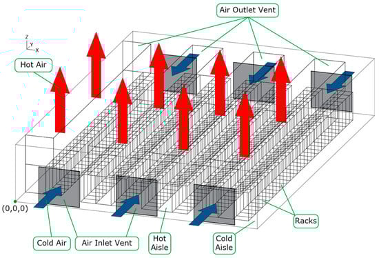
Figure 1.
The representation of three-dimensional geometry developed for the present study.
The computational mesh is composed of control volumes so that the equations of continuity, momentum and energy, presented in Section 2, could be solved. A mesh that has high quality is very important for the accomplishment of the simulations proposed in this paper, because this is fundamental for the numerical solution to converge and so that the achieved results are consistent and trustworthy. The resulting mesh consists of tetrahedral (cold corridors) and hexahedral (hot corridors and server racks) elements. This solution was adopted because the mesh would have a high number of control volumes if a mesh composed of only one type of elements were used. Additionally, as the air flow changes from horizontal direction when crossing the racks to vertical direction when going through the air outlet vent areas, the use of tetrahedral elements is required to reduce false mathematical diffusion and thus improve the accuracy of the numerical predictions. Figure 2 shows the mesh resulting from the study in an isometric perspective. Table 1 presents the characteristics of the computational mesh.

Figure 2.
The representation computational mesh in an isometric perspective.

Table 1.
Characteristics of the generated computational mesh.
The mesh density is an important metric and it is utilized for controlling accuracy and a high-density mesh delivers results with high accuracy. The meshes creation was an iterative process as its quality plays a significant role in the accuracy and stability of the numerical computation. The attributes associated with mesh quality are node point distribution, smoothness, and skewness. The quality of the mesh elements was assessed during the meshes creation in order to balance the results accuracy with the computational cost and simulation time. Three key parameters were analyzed to measure the mesh quality: aspect ratio, skewness and orthogonal quality. The aspect ratio is a measure of the stretching of a cell. It is computed as the ratio of the largest and smallest dimensions of the edges of the faces of the control volume. A good aspect ratio has a value close to one. Skewness is defined as the difference between the shape of the cell and the shape of an equilateral cell of equivalent volume. The mesh quality improves as skewness value approaches the null value. The orthogonal quality for cells is computed using the face normal vector, the vector from the cell centroid to the centroid of each of the adjacent cells, and the vector from the cell centroid to each of the faces. The orthogonal quality for a cell is computed as the minimum of these quantities. The mesh quality increases as the value of orthogonal quality is towards unity. Several computational meshes were created until the size of mesh elements provided a good aspect ratio, a small skewness and a good orthogonal quality, ensuring a good relation between the computational cost and the accuracy of the results. Although there are perceptible steps in the predictions of temperature and velocity fields, it is necessary to highlight that the selected meshes present a reasonable solution considering the results accuracy and the computational time required. Additionally, it must be noted that the numerical results simulate a real physical situation and their analysis and conclusions are in accordance with the computational resources required and computational time suitable for an engineering application.
The equations described in Section 2 were solved by a numerical process where the control volume technique was used. This technique is used when the differential equations have no analytical resolution and the numerical model must allow the discretization of the equations. To achieve a possible resolution of the numerical method, the computational domain was first divided into 2,341,172 control volumes. As stated above, a high-density mesh delivers results with high accuracy.
The second- order UpWind Scheme was applied to momentum, turbulent kinetic energy, turbulent dissipation rate, and energy to achieve more precise results. The accuracy of this method is reached on the faces of the control volumes by the expansion of the Taylor Series of the solution centered on the control volume compared to its centroid [42].
The PREssure STaggering Option (PRESTO!) interpolation method was used for pressure discretization. Its use is justified for controlling the sudden pressure variations between the centroids of the control volumes, considerable body forces, the presence of flows involving porous medium and other situations. It is based in the adoption of a staggered grid to calculate the pressure via a discrete continuity balance. In the staggered grid, the values of pressure in the center are known and these are the values at the interfaces in the normal grid. The PRESTO! scheme uses this technique, which resembles in characteristics the staggered-grid schemes used with structured meshes proposed by Patankar [42]. The Semi-Implicit Method for Pressure Linked Equations-Consistent (SIMPLEC) algorithm, published by Van Doormal and Raithby [43], was chosen in detriment to the Semi-Implicit Method for Pressure-Linked Equations (SIMPLE) algorithm for the pressure–velocity coupling [42], by allowing the convergence of the solution more quickly and ensuring the stability of the method.
3.1. Boundary Conditions
The boundary conditions defined in the numerical models were based on the data collected in the studied real data center. To the values collected was also added the value of pressure loss in the server racks, which are provided in [44].
It is important to point out that, from now on all, coordinate values and parameters are presented with dimensionless quantities to simplify the comparison between case studies. Dimensionless values are identified with a subscript “adm” in all equations of this study. The dimensionless quantities range from 0 to 1. It should be noted that, in the case of the temperature, the maximum value corresponds to a temperature value exceeding the operating specifications of the server racks. It is an air temperature value with the capacity to cause malfunctions or to damage to the equipment present in the ICT rooms, while this equipment is intended to operate uninterruptedly.
In this study, as previously mentioned, the PRESTO! interpolation method was used mainly due to the presence of porous medium [45]. The porous medium is an agglomerate of particles that are close, leaving small voids between them. Due to the existence of these voids, it is allowed to circulate liquid or gaseous elements that can fill them. Thus, the larger are these voids, the greater is the porosity of this material, that is, a greater amount of another element is required to fill them. In this study, only porosity was considered for the server racks, due to micro perforated doors that allow air to be introduced into the server rack. Besides the porosity present in the doors of the server rack, there are still the components inside that occupy the empty space inside the server rack, thus not allowing free air circulation. Therefore, for this study, the porosity of the server rack was considered as a whole (carcass and elements) and with the value of 80%, provided by the data center.
Due to the existence of porous media, it is necessary to calculate the coefficient of inertial loss “C2” applied to the server racks [45], which is given by the following expression:
where KL’ is the loss factor, Δp is the loss variation in Pa, and v is the velocity, in m·s−1. The coefficient of inertial loss, C2 is expressed as follows:
The coefficient of inertial loss (C2) is measured in m−1. For the resolution of Equation (10), the pressure variation value of 7.5 Pa was adjusted to the velocity of m·s−1 at the velocities present in [44].
The equations presented in Section 2 are solved in the fluid zone. The fluid zone was considered having an initial dimensionless temperature of 7.09 × 10⁻⁴, that is, the average dimensionless temperature measured within the ICT room.
The turbulence intensity and the hydraulic diameter are the parameters that allow the iterative calculation of the turbulent kinetic energy and the coefficient of dissipation of the turbulent kinetic energy. Regarding the intensity of turbulence, it indicates the direction of the flow. Generally it is considered 1% for low turbulence intensity and for high turbulence intensity it is considered 10% [45]. In this study, a turbulence intensity of 5% was considered in the extraction zone, as it is located in the containment zone of the hot aisles, which provides a well-defined direction of air flow. Concerning the intensity of turbulence in the air vent area, 5% was also considered since the air vent grids allow directing the air. These values were based on the experimental and numerical results provided in [46,47,48,49].
The boundary conditions are presented in Table 2 and are characterized by dimensionless values. The area of air vents presents values that are always equal, while in the extraction area different values occur, since one of the elements that compose this area is smaller.
Table 2.
Boundary conditions imposed in the air vent and extraction areas.
3.2. Solution Convergence
The convergence of the solution is obtained through the relaxation of the variables, decreasing the abrupt variations during the iteration. It is considered that a solution converges when all the residuals reach the stopping criterion, λ = 1 × 10⁻⁴ for all variables, except for the energy variable that assumes a stop criterion of λ = 1 × 10⁻⁶. In order for a solution to be considered convergent. there are several aspects to consider, such as refinement of the computational mesh, established numerical methods, relaxation factors and the number of imposed iterations. There are cases where it is not possible to achieve the convergence established by the stopping criterion, because the residuals stabilize before this criterion, thus assuming that the solution obtained is the possible convergence for the numerical method under analysis. The relaxation factors have no influence on the numerical solution’ they only change the time of the iterative process. Table 3 presents the various relaxation factors applied to the numerical methods, following the data provided in [46,47,48,49].
Table 3.
The relaxation factors applied to the numerical methods.
The iterative process of the various numerical models was defined for 1500 iterations, since the solution would not reach the stopping criteria, only if it could reach the possible convergence. The authors ran few scenarios with 7500 iterations, and no divergence was verified. However, due to the reason that these simulations took a high amount of time to compute, the authors decided to run the simulation up to 1500 iterations, since the variable residuals accomplished the possible convergence. Thus, this number of iterations was established to reduce the processing time of the simulation. Each case took about 14 h to complete all the iterations on a work station with two 3.47 GHz processors with 16 cores and with a memory of 48 GB of Random-access memory (RAM).
4. Description of the Modeled Case Studies
In this section, we present the parametric studies performed by changing different parameters that allowed the analysis of a good operation of an ICT room. For this analysis, the temperatures of the server racks and the hot aisles were studied, as well as the airflow in the ICT room. The investigated parametric studies differed among them, due to the variation of the thermal load of the server racks. Four case studies with different thermal loads were studied.
Cases 1 and 2 represent a usual thermal load distribution in the data center, especially Case 2. This objective was to have a study that closely resembles the reality of the operation of the server racks located in the data center. Meanwhile, Cases 3 and 4 represent a more academic approach. The thermal is not usually constant throughout the row since the servers do not usually operate at the same level of thermal load. However, the values of the thermal load in Cases 3 and 4 are close to the reality since these servers do not usually operate at maximum performance.
Each thermal load was simulated with the maximum and minimum air flow velocity. The dimensionless values are identified with a subscript “adm”. Figure 3 shows the upper plan view of the TI room, where the numbering corresponds to the server rack number, ranging from 1 to 208. In this figure, it is also possible to observe the hot aisle/cold aisle configuration of the data center. The smaller extraction aisle, mentioned in Table 3 and seen in Figure 3, is the one of the ranging racks from 181 until 208.
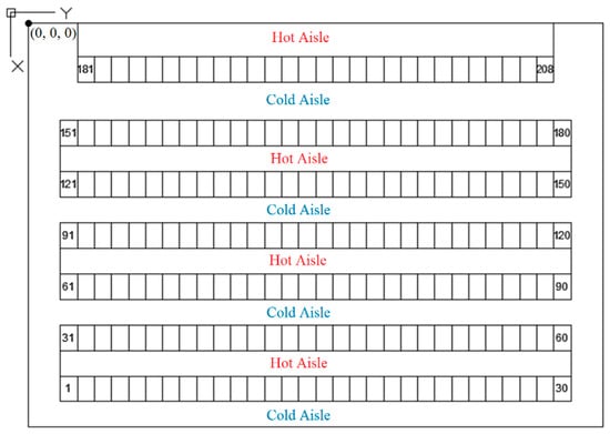
Figure 3.
The representation of upper plan view of the data center room.
In all four case studies addressed in this study, a dimensionless thermal load was used, qadm. In Case 1, different thermal loads imposed at the boundary conditions of the heat flow were applied symmetrically to every row of all server racks, as shown in Figure 4a. The thermal load is as follows: at the end of the rows of the server racks, 90% of the maximum thermal load was applied, while 70% of the maximum thermal load and 50% of the central racks were imposed on the intermediate server racks. For each case, the maximum and minimum air flow velocity was applied, simulated and studied. The purpose was to observe the behavior of the temperature and air flow in the room. To better understand how the loads were applied along the rows, a single row of server racks is shown in Figure 4 for each of the four case studies, where each color represents a value of the thermal load.
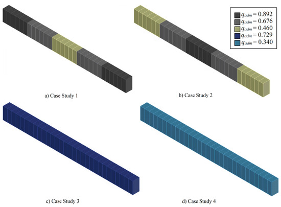
Figure 4.
The thermal load of the racks according to every case study.
Case 2 is similar to Case 1. However, in this case study, the thermal load applied on the end of the server racks is exchanged with the one of the central server racks, that is, the central server racks had a maximum heat load of 90% and the end server racks dissipated 50% of the maximum heat load. For Case 3, the thermal load applied was 75% of the maximum thermal load in the heat flow frontier condition, q. It was applied equally in every server rack, for the maximum and minimum velocity of the air flow. Finally, Case 4 is similar to Case 3, the difference being only the applied thermal load, which in this case was equal to the measured and nominal load value of the data center room.
5. Result Analysis
5.1. Case 1
In Case 1, several simulations were made with different thermal loads that were applied in the boundary conditions of the heat flow. The loads imposed were applied symmetrically along the rows, as shown in Figure 4a. The boundary conditions taken in account for these simulations are as follows: at the end of the rows of the server racks, 90% of the maximum thermal load was applied, while 70% of the maximum thermal load and 50% of the central racks were applied: qadm = 0.892 (90%), 0.676 (70%) and 0.460 (50%), respectively. The minimum air flow dimensionless velocity was set to be as follows: vadm = 0. By observing Figure 5 and Figure 6, the temperature field predictions of the y and z planes can be seen, respectively. These temperature fields predict the set of temperature values at all points in a given space at a given instant. For these specific cases, in steady-state conditions, the temperature field is independent of time.
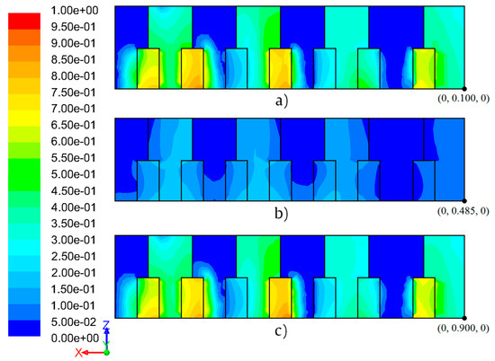
Figure 5.
The results of the field of temperature in the x-z plane through the planes: (a) yadm = 0.100; (b) yadm = 0.485; and (c) yadm = 0.900.
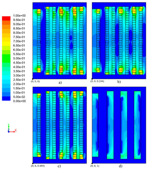
Figure 6.
The results of the field of temperature in the x-y plane through the planes: (a) zadm = 0; (b) zadm = 0.244; (c) zadm = 0.489; and (d) zadm = 1.
In the case of the maximum air flow dimensionless velocity, vadm = 1, the temperature field predictions can be seen in Figure 7 and Figure 8 for the y and z planes, respectively.
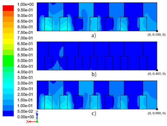
Figure 7.
The results of the field of temperature in the x–z plane through the planes: (a) yadm = 0.100; (b) yadm = 0.485; and (c) yadm = 0.900.
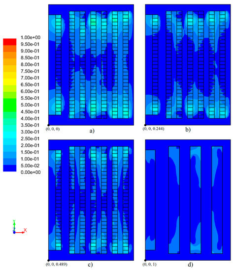
Figure 8.
The results of the field of temperature in the x–y plane through planes: (a) zadm = 0; (b) zadm = 0.244; (c) zadm = 0.489; and (d) zadm = 1.
More than a few hot spots are foreseen to arise at the termination of every server rack line, as illustrated in Figure 5 and Figure 6. These spots are easily spotted if noticing the colors related to the values which are higher than the dimensionless temperature, Tadm = 0.350, visible on the left scale, except for the hot spots in the extraction zone, which is Tadm = 0.125. Through a careful analysis of Figure 6a, a greater heat intensity is foreseen to occur at the bottom the racks located at the end ow every row. It can be deduced that the airflow is inadequate in this area. The justification behind this inadequacy is that the airflow intensity is higher in the center of the air vents than at the bottom and the top. Figure 6a–c also shows that for this case study hot spots can be predicted in the extraction zone and at the termination of all the rows.
In Figure 7a,c, which have server racks at the end of the rows (yadm = 0.100 and yadm = 0.900), the temperatures are expected to be very close to the hot spot limit, with Rack 2 exceeding that limit at the base. As far as the plan representing the central server racks is concerned (Figure 7b), it is expected that the temperature does not vary much from the inlet air temperature.
By observing Figure 8, it can be seen that there is a possibility of hot spots in a few server racks, such as racks located at the extremity of each row. As far as the extraction zone is concerned, the probability of hot spots is very high, since the mean temperatures shown in Figure 8d are very close to the inlet air temperature.
5.2. Case 2
In Case 2, the applied loads were applied symmetrically along the rows, as shown in Figure 4b. The boundary conditions set for the simulations performed in this studies are as follows: at the end of the rows of the server racks, 50% of the maximum thermal load was applied, while 70% of the maximum thermal load and 90% of the central racks were applied: qadm = 0.460 (50%), 0.676 (70%) and 0.892 (90%), respectively. The minimum air flow dimensionless velocity was set as follows: vadm = 0. The results from the simulations of the temperature field can be seen, respectively, in Figure 9 and Figure 10 for the y and z planes.
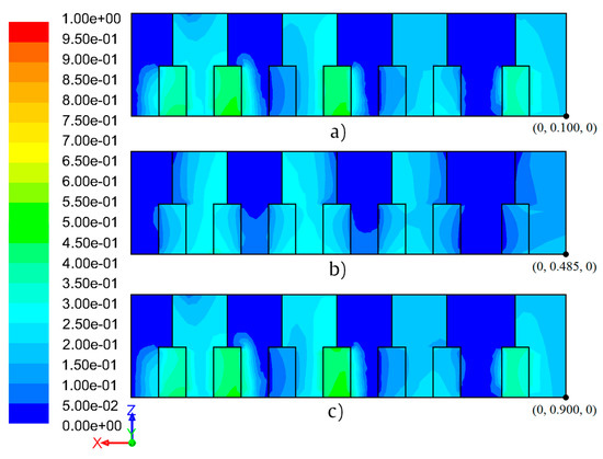
Figure 9.
The results of the field of temperature in the x–z plane through the planes: (a) yadm = 0.100; (b) yadm = 0.485; and (c) yadm = 0.900.
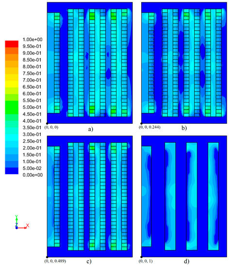
Figure 10.
The results of the field of temperature in the x–y plane through the planes: (a) zadm = 0; (b) zadm = 0.244; (c) zadm = 0.489; and (d) zadm = 1.
Figure 9 and Figure 10 show the temperature field predictions for the case study. The temperature fields are presented with the same planes as in Case 1.
By observing Figure 9, the probability of hot spots on the server racks can be accurately assessed. In the plans of Figure 9, it can also be easily noticed that the average of the non-dimensional temperature values in the extraction zone exceeds Tadm = 0.125. Therefore, the minimum air flow dimensionless velocity is not sufficient to successfully cool all the racks and, thus, avoid the occurrence of any type of hotspots.
By analyzing Figure 10, it can be seen that a few server racks can reach temperatures that exceed the minimum limit considered for a hot spot. In the extraction zone, the mean value of the dimensionless temperature in this zone is expected to exceed Tadm = 0.125 (the hot spot for this area), which means that hot spots in the extraction zone are very likely to occur.
In the case of the maximum level of air flow dimensionless velocity, vadm = 1, the results from the simulations of the temperature field can be seen, respectively, in Figure 11 and Figure 12 for the y and z planes.
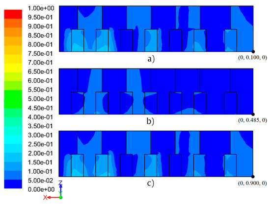
Figure 11.
The results of the field of temperature in the x–z plane through the planes: (a) yadm = 0.100; (b) yadm = 0.485; and (c) yadm = 0.900.
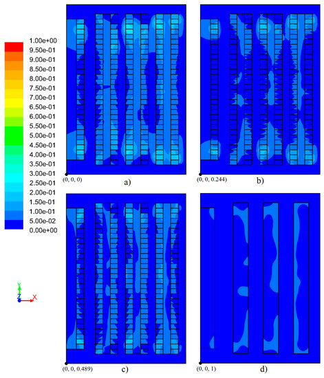
Figure 12.
The results of the field of temperature in the x–y plane through the planes: (a) zadm = 0; (b) zadm = 0.244; (c) zadm = 0.489; and (d) zadm = 1.
As shown in Figure 11b, the predicted dimensionless temperature does not exceed Tadm = 0.150. The zone that can reach this temperature is very small and very close to the base. In the other planes, the dimensionless temperature does not exceed Tadm = 0.200, which is also only reached at or near the base of the server racks.
Due to the increase in inlet air flow velocity, the temperature fields shown in Figure 12 predict that the average temperature in the data center room is similar to the inlet air temperature and that the formation of hot spots is almost non-existent, since the predicted maximum dimensionless temperature is Tadm = 0.250. As mentioned for Case 1, the hot spots can be easily spotted by noticing the colors related to the values, which are higher than the dimensionless temperature, Tadm = 0.350. In addition, no hot spots are expected in the extraction zone.
5.3. Case 3
For Case 3, the conditions of the boundary were set as follows: 75% of the maximum heat load in the heat flow boundary condition was imposed symmetrically, meaning that qadm = 0.729. As in previous cases, the minimum and maximum air flow velocity were applied. In the case of the minimum air flow velocity, the temperature field predictions can be seen, respectively, in Figure 13 and Figure 14 for the y and z planes.
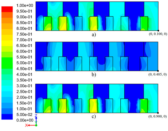
Figure 13.
The results of the field of temperature in the x–z plane through the planes: (a) yadm = 0.100; (b) yadm = 0.485; and (c) yadm = 0.900.
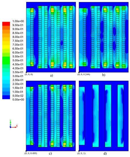
Figure 14.
The results of the field of temperature in the x–y plane through the planes: (a) zadm = 0; (b) zadm = 0.244; (c) zadm = 0.489; and (d) zadm = 1.
In Figure 13, it is possible to observe the temperature of the server racks above the established value for hot spots and average dimensionless temperatures in the hot aisles of Tadm = 0.350. Several hot spots occur with the minimum air flow velocity. It is possible to observe in Figure 14 that, for a minimum air flow velocity, when 75% is set for the maximum load, several hot spots are foreseen, as confirmed by Figure 13, in the server racks at the end of all the rows. Regarding the extraction temperature, an average dimensionless temperature around Tadm = 0.200 is expected, and, since it is higher than Tadm = 0.125, it leads to the prediction of hot spots.
When the air flow velocity is simulated at the maximum level, the temperature field predictions show a different result, as can be seen, respectively, in Figure 15 and Figure 16 for the y and z planes.
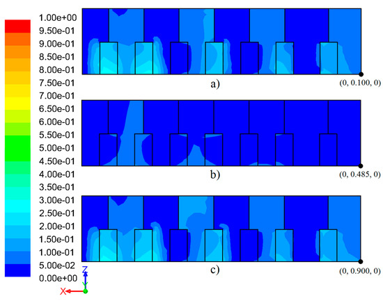
Figure 15.
The results of the field of temperature in the x–z plane through the planes: (a) yadm = 0.100; (b) yadm = 0.485; and (c) yadm = 0.900.
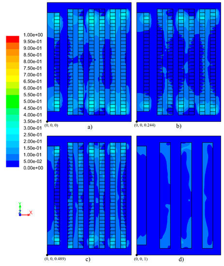
Figure 16.
The results of the field of temperature in the x–y plane through the: (a) zadm = 0; (b) zadm = 0.244; (c) zadm = 0.489; and (d) zadm = 1.
By observing Figure 15, it is possible to assess that some of the racks in the data center room exhibit temperature values similar to the inlet air temperature, especially in the intermediate server racks of each row.
As shown in the plane temperature fields of Figure 16, when applying the maximum level of air flow velocity, the thermal behavior of the data center room does not provide hot spots, neither for the server racks nor for the extraction zone, which has an average temperature similar to the inlet air temperature. Both figures confirm that no hot spots occur in this scenario.
5.4. Case 4
In Case 4, the nominal thermal load in the heat flow frontier condition, as mentioned in Section 4, and provided by the data center room, is qadm = 0.340. As in previous cases, the maximum and minimum air flow velocity were applied. The scale was changed for Case 4 and it does not present the maximum value existing in the other three cases. The reason is that this case study has lower temperatures and small differences would not be perceptible. By focusing on a narrower scale, it is possible to differentiate between slight changes in temperature.
The result of simulations for the minimum level of air flow velocity and the obtained temperature field predictions can be seen, respectively, in Figure 17 and Figure 18 for the y and z planes.
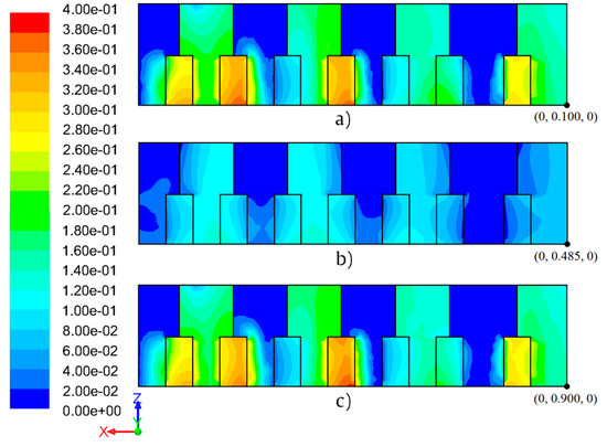
Figure 17.
The results of the field of temperature in the x–z plane through the planes: (a) yadm = 0.100; (b) yadm = 0.485; and (c) yadm = 0.900.
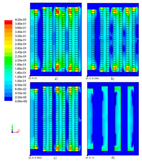
Figure 18.
The results of the field of temperature in the x–y plane through the planes: (a) zadm = 0; (b) zadm = 0.244; (c) zadm = 0.489; and (d) zadm = 1.
In the planes shown in Figure 17, it can be observed that the greater development of hot spots occurs at the terminations of the rows of the server racks. The temperature fields of the x–y planes (Figure 18) represent the temperature prediction for a usual thermal load with minimum air flow velocity. Due to the normal operation of the server racks, the air flow velocity is insufficient to avoid the formation of hot spots in several server racks. In the extraction zone, hot spots are not expected since the average dimensionless temperature does not exceed Tadm = 0.125.
By analyzing both Figure 17 and Figure 18, it can be assessed that the server racks at the end of the rows reach higher temperatures, meeting the dimensionless temperature value of Tadm = 0.400. The hot aisles are expected to reach the maximum average mean temperatures, Tadm = 0.120.
The result of simulations for the maximum level of air flow velocity and the obtained temperature field predictions can be seen, respectively, in Figure 19 and Figure 20 for the y and z planes.
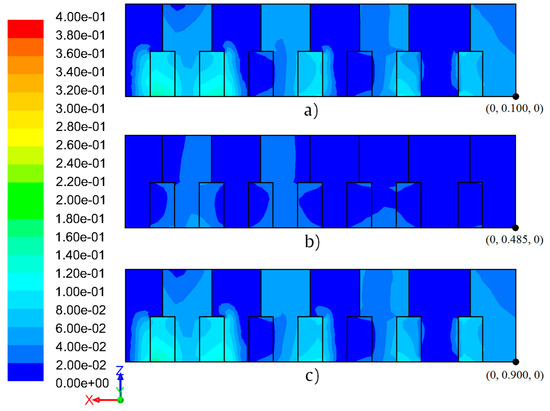
Figure 19.
The results of the field of temperature in the x–z plane through the planes: (a) yadm = 0.100; (b) yadm = 0.485; and (c) yadm = 0.900.
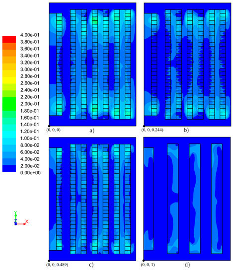
Figure 20.
The results of the field of temperature in the x–y plane through the planes: (a) zadm = 0; (b) zadm = 0.244; (c) zadm = 0.489; and (d) zadm = 1.
By observing Figure 19, it is possible to assess that the values obtained in the dimensionless temperature range of the server racks do not exceed the value, Tadm = 0.160. In the extraction zone, the simulations show that hot spots are not foreseen to occur, since the value of the dimensionless temperature field does not exceed the value of Tadm = 0.06.
Figure 20 shows the absence of hot spots, since the inlet air flow velocity proves to be oversized for this case study, which naturally leads to the prediction of low values in the extraction zone. It can be seen that server racks at the end of the rows are very close to the values of the central server racks, since the scale does not present the maximum value existing in the other three cases. Thus, it can be seen that there are no hot spots in any server rack. The value of the temperature range in the extraction zone is almost identical to that of the inlet air temperature.
5.5. The Velocity Vectors
A study of the velocity vectors is also presented in this subsection. In the four case studies addressed in this section, the minimum and maximum air flow velocity were applied, thus the behavior of the velocity vectors was equal in all of them. The only noticeable difference is in the minimum and maximum air flow velocity. Thus, only for these two cases are the velocity vectors illustrated. A representation of three-dimensional geometry of velocity vectors in the data center room can be observed in Figure 21.
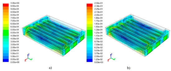
Figure 21.
The representation of three-dimensional geometry of velocity vectors for: (a) maximum air flow velocity; and (b) minimum air flow velocity.
5.5.1. Minimum Air Flow Velocity
In the case of the minimum air flow velocity, the velocity vectors predictions can be seen in Figure 22, Figure 23 and Figure 24 for the x, y and z planes, respectively.
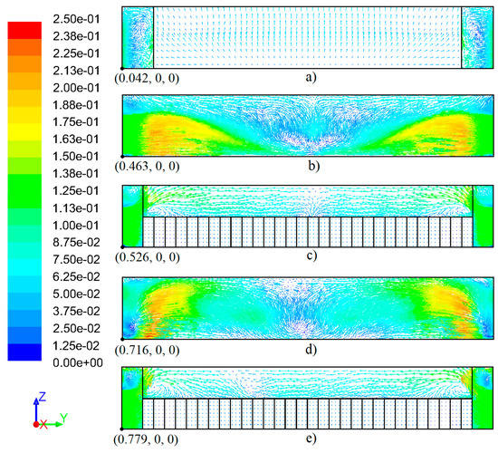
Figure 22.
The results of the dimensionless velocity vectors for the minimum air flow velocity in the y-z plane represented through the planes: (a) xadm = 0.042; (b) xadm = 0.116; (c) xadm = 0.526; (d) xadm = 0.589; (e) xadm = 0.779; and (f) xadm = 0.842.
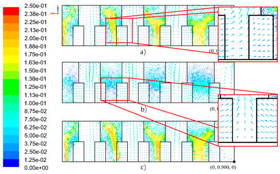
Figure 23.
The results of the dimensionless velocity vectors for the minimum air flow velocity in the x–z plane represented through the planes: (a) yadm = 0.100; (b) yadm = 0.485; and (c) yadm = 0.900.
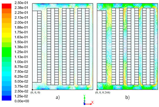
Figure 24.
The results of the dimensionless velocity vectors for the minimum air flow velocity in the x–y plane represented through the planes: (a) zadm = 0; and (b) zadm = 0.244.
It is possible to observe in Figure 22b,d for xadm = 0.463 and xadm = 0.716 that near the inlet air flow vent the air collides with the plates at the extremity of the server racks. Thus, it becomes noticeable that the air flow gains speed at the end of each row.
By observing Figure 23a–c, it is expected that air recirculation will occur in some racks. This is due to the difficulty that air has in entering them, since the injected inlet air collides with the plates at the extremity of the server racks as mentioned above. In Figure 23b, it is predicted that the air flow will follow the desirable path. In this plan, it is possible to understand the behavior of the air flow in most of the server racks present in the data center room. It can be seen in the hot aisles that the prediction of the flow direction of the air exiting the server racks follows the desirable path to the extraction zone, with the exception of the air adjacent to the ends of the aisles, which tends to enter the exit of the server racks.
By observing Figure 24a,b, it is predicted that, in the mid-height of the inlet air flow vent area, more pronounced values of air velocity can be noticed. In the inlet air flow vent area, vortices and small air recirculation are expected to occur due to the amount of movement blown in by the air vents. Air is still expected to be diverted from the desirable path towards the cold aisles as it collides with the plates at the extremity of the server racks and with the containment doors. Due to deviations in the trajectory, the air increases its velocity at the beginning of the cold aisles, gradually losing it as it moves towards the center of the cold aisle. It is also predicted that the floor and ceiling of the data center room will experience slower air flow velocities.
5.5.2. Maximum Air Flow Velocity
In the case of the maximum air flow velocity, the velocity vectors predictions can be seen, respectively, in Figure 25, Figure 26 and Figure 27 for the x, y and z planes.
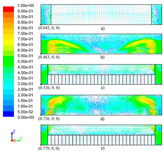
Figure 25.
The results of the dimensionless velocity vectors for the maximum air flow velocity in the y–z plane represented through the planes (a) xadm = 0.042; (b) xadm = 0.116; (c) xadm = 0.526; (d) xadm = 0.589; (e) xadm = 0.779.
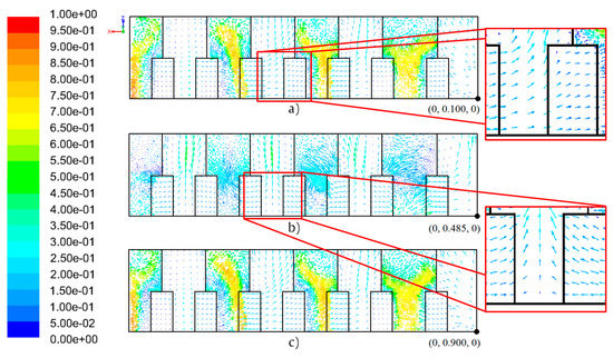
Figure 26.
The results of the dimensionless velocity vectors for the maximum air flow velocity in the x–z plane represented through the planes: (a) yadm = 0.100; (b) yadm = 0.485; and (c) yadm = 0.900.
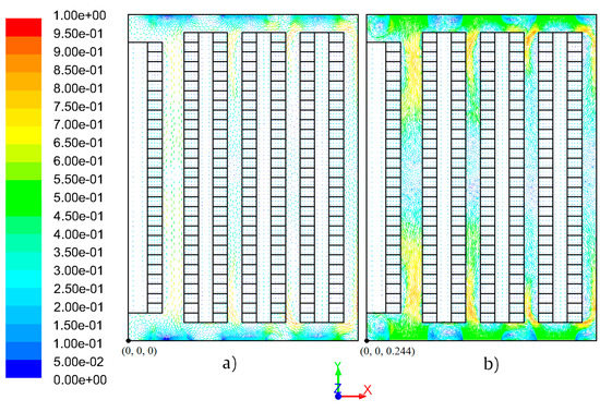
Figure 27.
The results of the dimensionless velocity vectors for the maximum air flow velocity in the x–y plane represented through the planes: (a) zadm = 0; and (b) zadm = 0.244.
In this case, the prediction is very similar to that of the minimum air flow velocity, since the air flow behaves in the same way. However, in this case, the velocity of the air flow is higher than the minimum air flow velocity scenario. Figure 25 and Figure 27 indicate that the behavior of the air flow is similar to the minimum air flow velocity scenario. Figure 26 shows the prediction of airflow in the hot aisles. It can be seen that in these planes the air in the center of the hot aisles is correctly directed to the extraction zone, as it can be seen in Figure 26b. However, at the end of the hot aisles, as seen in Figure 26a,c, the air has a horizontal direction, since in the server racks at the end, the flow is made in reverse because the problem mentioned in Section 5.5.1 occurs in the cold aisles. Figure 25b,d and Figure 27b demonstrate the prediction of the air flow velocity increases since near the inlet air flow vent the air collides with the plates at the extremity of the server racks. Due to the increase of this velocity, the air near the server racks located at the end experiences circulation difficulties.
The results show that the airflow could be better close to the end of the rows of the server racks. Such a phenomenon occurs because the layout of the data center room is imperfect. This imperfect cooling can be noticed by observing the enhanced section of Figure 26a, where the air inadequately flows, from the hot aisle, in the direction of the cold aisle. Nevertheless, as reinforced by the information conveyed by the planes in Figure 25 and Figure 27, the cooling is significantly more efficient in the middle of the room, as demonstrated by the air flow represented in the enhanced section of Figure 26b, in which the air adequately flows in the direction of the hot aisle from the cold aisle.
5.6. Result Discussion and Analysis
Due to changes in the boundary conditions imposed on the heat flow and the different applied air flow velocities, the case studies differ with respect to the temperature fields, which can cause a few hot spots in the server racks. Figure 28 represents the maximum dimensionless temperature predicted in each case study. In this figure, the temperature limit of hot spots in the server racks can be observed. When analyzing the case studies and Figure 28, it is predicted that not all generate hot spots in server racks, especially in the cases with the maximum air flow velocity.
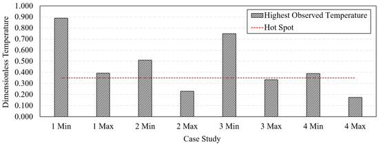
Figure 28.
The maximum dimensionless temperature predicted in each case study for the maximum level and minimum level of air flow velocity.
In this sense, it is possible to reduce the thermal load of the server racks by improving the overall thermal performance of the processing room, without jeopardizing the correct operation of the server racks located in the sensible regions of the data center room and increasing the sustainability of the entire data center. It can also be observed that Case 4 is the one that displays the best behavior and in which there is a lower probability of hot spot occurrence.
As stated in Section 4, the maximum airflow dimensionless velocity, vadm, is 1, a velocity that is not a common practice in the studied data center. The velocity is set only in cases when the demand for the rack services and operation is greater than usual and the larger part of the racks function at full capacity. By setting the CRAC units to a maximum airflow velocity, the data center room can be successfully cooled, yet this refrigeration is achieved at a high cost since it is accomplished through the consumption of a high quantity of energy. Thus, as an alternative to upgrading the existing CRAC units, which could signify high expenses, a possible and more sustainable resolution can be altering the way the racks are arranged inside the data center room. The purpose is optimizing the existing layout with the aim of efficiently refrigerating the server racks. One of these alterations could be the removal of a few server racks located at the extremity of the line and consequently avoiding hot spots by improving the air flow.
6. Conclusions
A parametric study was made by employing CFD modeling for a real data center room comprising more than 200 server racks with the purpose of studying the thermal performance and airflow. Four case studies with distinct thermal loads were addressed in this study. Several scenarios were simulated for the heat flow limit condition and the results for four case studies were obtained and then analyzed for the maximum and minimum air flow velocity. The main results are as follows:
- For all four case studies, the results predict the occurrence of several hot spots in the case of the minimum air flow velocity.
- By analyzing the results, no hot spots materialize in the case of the maximum air flow velocity except in Case 1.
- Case 4 shows the best solution. Conversely, refrigerating through these means is unsustainable and consumes a great amount of energy.
- From the results, it can also be deduced that every predicted hot spot is situated at the end of the aisles. The reason behind this occurrence is the ineffective refrigeration of the data center server racks as a result of an inappropriate position of the CRAC units and this happens in every case study.
- Having to always use the maximum air flow velocity, as in Cases 1–3, is not the best solution. The airflow is suboptimal close to the end of the rows since the layout of the data center room is imperfect. This challenge can be overcome by withdrawing a few server racks located at the end of the aisles. Such a solution could signify a much better airflow and could even allow a reduction of the air flow velocity, thus diminishing the overall cost with entire cooling operation.
Author Contributions
D.M.: Writing and simulating original paper; R.G.: conceptualization, methodology and revising; P.D.G.: editing, data analyzing, funding acquisition, supervision; P.D.d.S: editing, M.T.C.: revising the paper, validation.
Funding
The current study was funded in part by Fundação para a Ciência e Tecnologia (FCT), under project UID/EMS/00151/2019 C-MAST, with reference POCI-01-0145-FEDER-007718. Radu Godina would like to acknowledge the financial support from Fundação para a Ciência e Tecnologia (FCT), (grant UID/EMS/00667/2019).
Conflicts of Interest
The authors declare no conflict of interest.
References
- Deymi-Dashtebayaz, M.; Valipour-Namanlo, S. Thermoeconomic and environmental feasibility of waste heat recovery of a data center using air source heat pump. J. Clean. Prod. 2019, 219, 117–126. [Google Scholar] [CrossRef]
- Abdullah, M.; Lu, K.; Wieder, P.; Yahyapour, R. A Heuristic-Based Approach for Dynamic VMs Consolidation in Cloud Data Centers. Arab. J. Sci. Eng. 2017, 42, 3535–3549. [Google Scholar] [CrossRef]
- Ni, J.; Jin, B.; Zhang, B.; Wang, X. Simulation of Thermal Distribution and Airflow for Efficient Energy Consumption in a Small Data Centers. Sustainability 2017, 9, 664. [Google Scholar] [CrossRef]
- Cho, K.; Chang, H.; Jung, Y.; Yoon, Y. Economic analysis of data center cooling strategies. Sustain. Cities Soc. 2017, 31, 234–243. [Google Scholar] [CrossRef]
- Pärssinen, M.; Wahlroos, M.; Manner, J.; Syri, S. Waste heat from data centers: An investment analysis. Sustain. Cities Soc. 2019, 44, 428–444. [Google Scholar] [CrossRef]
- El Kafhali, S.; Salah, K. Modeling and Analysis of Performance and Energy Consumption in Cloud Data Centers. Arab. J. Sci. Eng. 2018, 43, 7789–7802. [Google Scholar] [CrossRef]
- Grange, L.; Da Costa, G.; Stolf, P. Green IT scheduling for data center powered with renewable energy. Future Gener. Comput. Syst. 2018, 86, 99–120. [Google Scholar] [CrossRef]
- AL-Hazemi, F.; Peng, Y.; Youn, C.-H.; Lorincz, J.; Li, C.; Song, G.; Boutaba, R. Dynamic allocation of power delivery paths in consolidated data centers based on adaptive UPS switching. Comput. Netw. 2018, 144, 254–270. [Google Scholar] [CrossRef]
- Fernández-Cerero, D.; Fernández-Montes, A.; Ortega, J.A. Energy policies for data-center monolithic schedulers. Expert Syst. Appl. 2018, 110, 170–181. [Google Scholar] [CrossRef]
- Díaz, A.J.; Cáceres, R.; Cardemil, J.M.; Silva-Llanca, L. Energy and exergy assessment in a perimeter cooled data center: The value of second law efficiency. Appl. Therm. Eng. 2017, 124, 820–830. [Google Scholar] [CrossRef]
- Oró, E.; Taddeo, P.; Salom, J. Waste heat recovery from urban air cooled data centres to increase energy efficiency of district heating networks. Sustain. Cities Soc. 2019, 45, 522–542. [Google Scholar] [CrossRef]
- Dandres, T.; Farrahi Moghaddam, R.; Nguyen, K.K.; Lemieux, Y.; Samson, R.; Cheriet, M. Consideration of marginal electricity in real-time minimization of distributed data centre emissions. J. Clean. Prod. 2017, 143, 116–124. [Google Scholar] [CrossRef]
- Andrae, A.S.G.; Edler, T. On Global Electricity Usage of Communication Technology: Trends to 2030. Challenges 2015, 6, 117–157. [Google Scholar] [CrossRef]
- Lu, H.; Zhang, Z.; Yang, L. A review on airflow distribution and management in data center. Energy Build. 2018, 179, 264–277. [Google Scholar] [CrossRef]
- Nada, S.A.; Said, M.A.; Rady, M.A. Numerical investigation and parametric study for thermal and energy management enhancements in data centers’ buildings. Appl. Therm. Eng. 2016, 98, 110–128. [Google Scholar] [CrossRef]
- Rong, H.; Zhang, H.; Xiao, S.; Li, C.; Hu, C. Optimizing energy consumption for data centers. Renew. Sustain. Energy Rev. 2016, 58, 674–691. [Google Scholar] [CrossRef]
- Oró, E.; Allepuz, R.; Martorell, I.; Salom, J. Design and economic analysis of liquid cooled data centres for waste heat recovery: A case study for an indoor swimming pool. Sustain. Cities Soc. 2018, 36, 185–203. [Google Scholar] [CrossRef]
- Nada, S.A.; Attia, A.M.A.; Elfeky, K.E. Experimental study of solving thermal heterogeneity problem of data center servers. Appl. Therm. Eng. 2016, 109, 466–474. [Google Scholar] [CrossRef]
- Fakhim, B.; Behnia, M.; Armfield, S.W.; Srinarayana, N. Cooling solutions in an operational data centre: A case study. Appl. Therm. Eng. 2011, 31, 2279–2291. [Google Scholar] [CrossRef]
- Peng, G.; Zhou, C.; Wang, S. Model Predictive Control of Data Center Temperature Based on CFD. In Bio-inspired Computing: Theories and Applications; Qiao, J., Zhao, X., Pan, L., Zuo, X., Zhang, X., Zhang, Q., Huang, S., Eds.; Springer: Singapore, 2018; pp. 423–433. [Google Scholar]
- Deshmukh, A.N.; Pawar, R.S.; Kulkarni, S.S.; Kumar, V.; Joshi, S.K.; Chaudhari, M.B. CFD Simulation Studies of High Performance Computing (HPC) Facilities. In Fluid Mechanics and Fluid Power—Contemporary Research; Saha, A.K., Das, D., Srivastava, R., Panigrahi, P.K., Muralidhar, K., Eds.; Springer: Pune, India, 2017; pp. 251–267. [Google Scholar]
- Wibron, E.; Ljung, A.-L.; Lundström, T.S. Computational Fluid Dynamics Modeling and Validating Experiments of Airflow in a Data Center. Energies 2018, 11, 644. [Google Scholar] [CrossRef]
- Habibi Khalaj, A.; Halgamuge, S.K. A Review on efficient thermal management of air- and liquid-cooled data centers: From chip to the cooling system. Appl. Energy 2017, 205, 1165–1188. [Google Scholar] [CrossRef]
- Zhang, K.; Zhang, Y.; Liu, J.; Niu, X. Recent advancements on thermal management and evaluation for data centers. Appl. Therm. Eng. 2018, 142, 215–231. [Google Scholar] [CrossRef]
- Athavale, J.; Yoda, M.; Joshi, Y. Chapter Three—Thermal Modeling of Data Centers for Control and Energy Usage Optimization. In Advances in Heat Transfer; Sparrow, E.M., Abraham, J.P., Gorman, J.M., Eds.; Elsevier: Amsterdam, The Netherlands, 2018; Volume 50, pp. 123–186. [Google Scholar]
- Nadjahi, C.; Louahlia, H.; Lemasson, S. A review of thermal management and innovative cooling strategies for data center. Sustain. Comput. Inform. Syst. 2018, 19, 14–28. [Google Scholar] [CrossRef]
- López, V.; Hamann, H.F. Heat transfer modeling in data centers. Int. J. Heat Mass Transf. 2011, 54, 5306–5318. [Google Scholar] [CrossRef]
- Almoli, A.; Thompson, A.; Kapur, N.; Summers, J.; Thompson, H.; Hannah, G. Computational fluid dynamic investigation of liquid rack cooling in data centres. Appl. Energy 2012, 89, 150–155. [Google Scholar] [CrossRef]
- Song, Z. Thermal performance of a contained data center with fan-assisted perforations. Appl. Therm. Eng. 2016, 102, 1175–1184. [Google Scholar] [CrossRef]
- Nada, S.A.; Said, M.A. Comprehensive study on the effects of plenum depths on air flow and thermal managements in data centers. Int. J. Therm. Sci. 2017, 122, 302–312. [Google Scholar] [CrossRef]
- Xie, M.; Wang, J.; Liu, J. Evaluation metrics of thermal management in data centers based on exergy analysis. Appl. Therm. Eng. 2019, 147, 1083–1095. [Google Scholar] [CrossRef]
- Nada, S.A.; Said, M.A.; Rady, M.A. CFD investigations of data centers’ thermal performance for different configurations of CRACs units and aisles separation. Alex. Eng. J. 2016, 55, 959–971. [Google Scholar] [CrossRef]
- Chu, W.-X.; Hsu, C.-S.; Tsui, Y.-Y.; Wang, C.-C. Experimental investigation on thermal management for small container data center. J. Build. Eng. 2019, 21, 317–327. [Google Scholar] [CrossRef]
- Ullah, R.; Ahmad, N.; Malik, S.U.R.; Akbar, S.; Anjum, A. Simulator for modeling, analysis, and visualizations of thermal status in data centers. Sustain. Comput. Inform. Syst. 2018, 19, 324–340. [Google Scholar] [CrossRef]
- Nada, S.A.; Said, M.A. Effect of CRAC units layout on thermal management of data center. Appl. Therm. Eng. 2017, 118, 339–344. [Google Scholar] [CrossRef]
- Song, Z. Studying the fan-assisted cooling using the Taguchi approach in open and closed data centers. Int. J. Heat Mass Transf. 2017, 111, 593–601. [Google Scholar] [CrossRef]
- Pritchard, P.J. Fox and McDonald’s Introduction to Fluid Mechanics, 8th ed.; Binder Ready Version Edition; Wiley: Hoboken, NJ, USA, 2011; ISBN 978-1-118-35599-2. [Google Scholar]
- Norton, T.; Sun, D.-W. Computational fluid dynamics (CFD)—An effective and efficient design and analysis tool for the food industry: A review. Trends Food Sci. Technol. 2006, 17, 600–620. [Google Scholar] [CrossRef]
- Cho, J.; Lim, T.; Kim, B.S. Measurements and predictions of the air distribution systems in high compute density (Internet) data centers. Energy Build. 2009, 41, 1107–1115. [Google Scholar] [CrossRef]
- Alkharabsheh, S.; Fernandes, J.; Gebrehiwot, B.; Agonafer, D.; Ghose, K.; Ortega, A.; Joshi, Y.; Sammakia, B. A Brief Overview of Recent Developments in Thermal Management in Data Centers. J. Electron. Packag. 2015, 137. [Google Scholar] [CrossRef]
- Hoang, M.L.; Verboven, P.; De Baerdemaeker, J.; Nicolaï, B.M. Analysis of the air flow in a cold store by means of computational fluid dynamics. Int. J. Refrig. 2000, 23, 127–140. [Google Scholar] [CrossRef]
- Patankar, S. Numerical Heat Transfer and Fluid Flow, 1st ed.; CRC Press: New York, NY, USA, 1980; ISBN 978-0-89116-522-4. [Google Scholar]
- Doormaal, J.P.V.; Raithby, G.D. Enhancements of the Simple Method for Predicting Incompressible Fluid Flows. Numer. Heat Transf. 1984, 7, 147–163. [Google Scholar]
- North, T. Understanding How Cabinet Door Perforation Impacts Airflow. BICSI News Mag. 2011, 36–42. [Google Scholar]
- Ansys Fluent 14.0: Users Guide; Release 14.0; ANSYS, Inc.: Canonsburg, PA, USA, 2011.
- Gaspar, P.D.; Gonçalves, L.C.; Pitarma, R.A. Experimental analysis of the thermal entrainment factor of air curtains in vertical open display cabinets for different ambient air conditions. Appl. Therm. Eng. 2011, 31, 961–969. [Google Scholar] [CrossRef]
- Gaspar, P.D.; Gonçalves, L.C.C.; Pitarma, R.A. Detailed CFD Modelling of Open Refrigerated Display Cabinets. Available online: https://www.hindawi.com/journals/mse/2012/973601/ (accessed on 22 January 2019).
- Gaspar, P.D.; Carrilho Gonçalves, L.C.; Pitarma, R.A. CFD Parametric Studies for Global Performance Improvement of Open Refrigerated Display Cabinets. Available online: https://www.hindawi.com/journals/mse/2012/867820/ (accessed on 22 January 2019).
- Carneiro, R.; Gaspar, P.D.; Silva, P.D. 3D and transient numerical modelling of door opening and closing processes and its influence on thermal performance of cold rooms. Appl. Therm. Eng. 2017, 113, 585–600. [Google Scholar] [CrossRef]
© 2019 by the authors. Licensee MDPI, Basel, Switzerland. This article is an open access article distributed under the terms and conditions of the Creative Commons Attribution (CC BY) license (http://creativecommons.org/licenses/by/4.0/).