Abstract
Recently, deep learning technology has been applied to medical images. This study aimed to create a detector able to automatically detect an anatomical structure presented in a brain magnetic resonance imaging (MRI) scan to draw a standard line. A total of 1200 brain sagittal MRI scans were used for training and validation. Two sizes of regions of interest (ROIs) were drawn on each anatomical structure measuring 64 × 64 pixels and 32 × 32 pixels, respectively. Data augmentation was applied to these ROIs. The faster region-based convolutional neural network was used as the network model for training. The detectors created were validated to evaluate the precision of detection. Anatomical structures detected by the model created were processed to draw the standard line. The average precision of anatomical detection, detection rate of the standard line, and accuracy rate of achieving a correct drawing were evaluated. For the 64 × 64-pixel ROI, the mean average precision achieved a result of 0.76 ± 0.04, which was higher than the outcome achieved with the 32 × 32-pixel ROI. Moreover, the detection and accuracy rates of the angle of difference at 10 degrees for the orbitomeatal line were 93.3 ± 5.2 and 76.7 ± 11.0, respectively. The automatic detection of a reference line for brain MRI can help technologists improve this examination.
1. Introduction
The convolutional neural network (CNN) [1] can be trained to extract image features via multiple layers. There are so many types of CNN models [2,3,4] to choose from and new methods being published and discussed. The object detection technique with CNN [5,6,7,8] can detect the locations of regions of interest by distinguishing them from the background, although the image classification with CNN can be classified to specific categories as the whole of an image. Recently, deep learning technology has been adopted in many areas, including image classification [2,3,4], object detection [5,6,7,8], and image segmentation [9]. These deep learning technologies have also been applied to medical images. Examples include computed tomography image classification [10,11], feature extraction [12,13] and automatic detection of lung tumors [14,15], and automatic detection of breast tumors on X-ray images [16,17]. These machine-aided diagnostic techniques have supported the efforts of radiologists to achieve more accurate diagnoses and tumor detection. However, no medical image acquisition technique incorporating deep learning is currently available at this time. Magnetic resonance imaging (MRI) of the brain is one of the most common image acquisitions performed in the hospital. The acquisition of brain MRI scans involves obtaining an arbitrary cross section without radiation exposure. However, determining the ideal angle of the sections is necessary to be able to acquire an arbitrary cross section easily. Currently, some standard lines for brain MRI exist, such as the orbitomeatal line (OM-line) [18] and the anterior commissure–posterior commissure line (AC-PC line) [19]. The use of these standard lines facilitates the location of specific anatomical structures by the technologists manually. The model-based detection [20] for the AC and PC have been reported to dealing with detections of anatomies. However, the anatomies for the OM line could not be supported in this technique. Therefore, the automatic detection of the standard line using a deep learning technique would be useful for technologists seeking to acquire brain MRI scans. The purpose of the present study was to detect standard lines automatically for brain MRI using a deep learning technique.
2. Materials and Methods
2.1. Subjects and MRI Scans
The study included 1200 patients (585 males and 615 females, mean age ± standard deviation (SD): 55.8 ± 20.1 years) who were subjected to an MRI examination of the brain between September and November 2016 at Hokkaido University Hospital. All MRI images were obtained using two 1.5-tesla (T) MRI scanners (the Achieva A-series from Philips Healthcare, Best, the Netherlands, or the MAGNETOM Avanto from Siemens Healthcare, Erlangen, Germany) and three 3-T MRI scanners (the GE Discovery MR 750 w from GE Healthcare, Chicago, IL, USA, the TRILLIUM OVAL from Hitachi, Tokyo, Japan, or the Achieva TX from Philips Healthcare, Best, the Netherlands). The direction of the slice in this study incorporated the median sagittal plane. This study was approved by the ethics committee of Hokkaido University Hospital.
2.2. Datasets and Preprocessing of Images
The MRI scans were retrieved from the picture archiving and communication system. To convert the images for use by the training database, they were converted from the Digital Imaging and Communications in Medicine (DICOM) format to the Joint Photographic Experts Group (JPEG) format using a dedicated DICOM software (XTREK view, J-MAC SYSTEM Inc., Sapporo, Japan). The window width and level of the DICOM images were used to preset values in the DICOM tag. The DICOM images were converted to JPEG images with a size of 512 × 512 pixels. The size of the image was unified for inputting as the same size in the software because the middle sagittal images in this study were obtained by several different MRI scanners. JPEG files were loaded into the in-house MATLAB software program (The MathWorks, Inc., Natick, MA, USA). The software was used to draw regions of interest (ROIs) with sizes of 64 × 64 pixels and 32 × 32 pixels at the center of specific structures. The ROIs were drawn according to the anatomies of the root of the nose (Nose), inferior border of the pons (Pons), the AC, and the PC (Figure 1). The ROI data were outputted as a text file, which included the object name, coordinates, and size of each ROI. The dataset was divided into six subsets to complete the six-fold cross-validation. Two hundred images were included in each subset, with a total of five subsets (1000 images) used for training and the other five subsets used for validation (Figure 2). Data augmentation [21,22] was performed involving 1000 images for the improvement of the training. The training images were applied as a data augmentation dataset to the image rotation, which involved angles from −30 to 30 degrees in 3-degree steps (Figure 3).
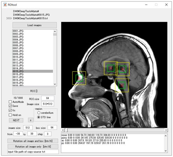
Figure 1.
The software for training outlined ROIs over the noteworthy anatomical characteristics. The red circle is the center of the target anatomy, the yellow bounding boxes are the ROIs measuring 64 × 64 pixels, and the green bounding boxes are the ROIs measuring 32 × 32 pixels.
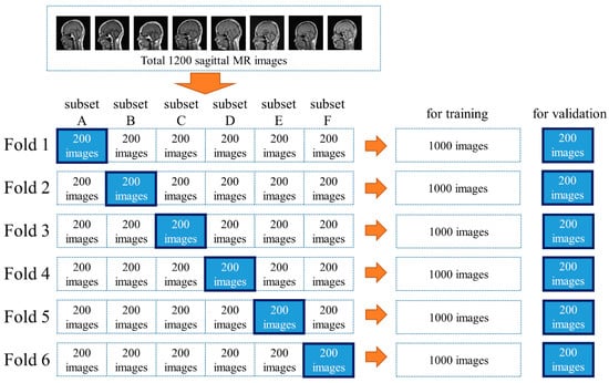
Figure 2.
A total of 1200 images were divided into six subsets to complete the six-fold cross-validation.
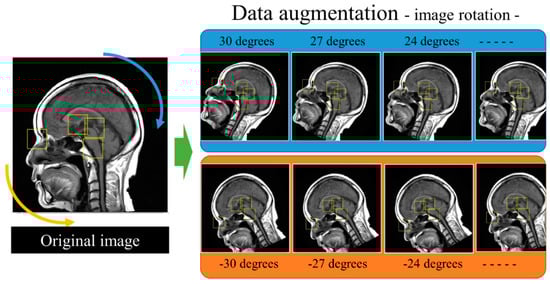
Figure 3.
The procedure for data augmentation of the training datasets. The original images and supervised bounding boxes were rotated from −30 to 30 degrees in 3-degree steps.
2.3. Training of the Images for Model Creation
The software for the deep learning technique was developed via in-house MATLAB software, and a deep learning–optimized machine with a Nvidia GeForce GTX 1080 Ti graphics card (Nvidia Corporation, Santa Clara, CA, USA), with 11.34 tera floating point operations per second (TFLOPS) of single-precision performance, 484 GB/s of memory bandwidth, and 11 GB of memory per board was used. The image training was performed using the faster region-based convolutional neural network (R-CNN) [8] with the Computer Vision System Toolbox on the MATLAB software. Training was divided into four steps inside the MATLAB software. During the first two steps, the region proposal and detection networks were created, while the latter two steps were performed together to train the networks for detection. The hyper-parameters of the training models were as follows: Maximum training epochs, 10; initial learning rates, 0.00001 (first two steps) and 0.000001 (latter two steps); and mini batch size, 1. The stochastic gradient descent with momentum (SGDM) was used for optimization with an initial learning rate. The momentum set to 0.9 and L2 regulation set to 0.0001. Image training was performed six times according to the training datasets in Figure 2.
2.4. Evaluation of the Created Models and a Standard Line for Brain MRI
The predicted bounding boxes were incorporated into the MATLAB software to show only one box representing the area with the highest confidence for each anatomy. The detection of different anatomies was evaluated using the average precision (AP) and the mean average precision (mAP) [23]. The ROIs measuring 64 × 64 pixels and 32 × 32 pixels, respectively, were evaluated separately. The higher mAP among the two ROI sizes was selected to evaluate for comparison with the standard lines of the brain imaging, that is, the OM-line and the AC-PC line. The delineation of a standard line for brain MRI was calculated using the MATLAB software (Figure 4). The standard lines were calculated by using the central coordinate of the predicted bounding boxes. If there was no detection of the bounding boxes, which is a necessary requirement to draw the standard line, the line was not represented in the software. The software also had a function of calculating the angle of the predicted line that was formed at an angle relative to the horizontal direction of the image. The number of the predicted lines was calculated as a line-detection rate. The accuracy rates of the delineation for the standard line were calculated to obtain the difference between the original and prediction angles among the detected lines. The processing speeds by calculating the computation time per image were also measured. The angles were evaluated from 0.5 to 10.0 degrees of the absolute value of the angles. All the results were represented as means and SDs according to the number of six-fold datasets.
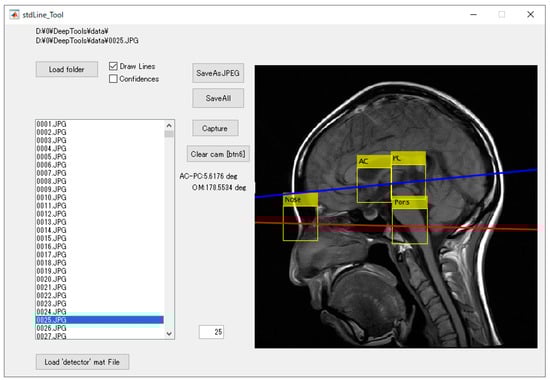
Figure 4.
The detection software based on the created model and the delineation of the standard line for brain magnetic resonance imaging (MRI). The yellow bounding boxes represent automatically detected anatomy, the red line is the calculated orbitomeatal (OM)-line, and the blue line is the calculated anterior commissure–posterior commissure (AC-PC) line.
3. Results
3.1. The Detection of Anatomies
Table 1 and Table 2 show the AP and mAP for the ROI sizes of 64 × 64 pixels and 32 × 32 pixels, respectively. The mAP for the ROIs measuring 64 × 64 pixels was 0.76 ± 0.04, which was higher than those for the ROIs measuring 32 × 32 pixels. Separately, for the ROIs measuring 64 × 64 pixels, the AP of the Nose (0.85 ± 0.07), Pons (0.78 ± 0.11), PC (0.74 ± 0.05), and AC (0.68 ± 0.04) were calculated in the higher order. There was no AP value over 0.5 for the ROIs measuring 32 × 32 pixels in each anatomy.

Table 1.
Average precision (AP) and mean average precision (mAP) for the ROIs measuring 64 × 64 pixels.
Table 2.
AP and mAP for the ROIs measuring 32 × 32 pixels.
3.2. Line-Detection Rates and Accuracies
Table 3 shows the line-detection rates for the brain MRI scans. The detection rate of the OM-line was higher than the AC-PC line. Figure 5 shows the accuracy rates of the delineation for the standard line. The angles of difference at 3, 5, and 10 degrees for the OM-line between the original and predicted lines were 57.5 ± 10.9, 69.8 ± 11.2, and 76.7 ± 11.0, respectively. Additionally, the angles of differences at 3, 5, and 10 degrees for the AC-PC line between the original and predicted lines were 21.7 ± 4.6, 31.6 ± 4.3, and 47.1 ± 5.0, respectively. Table 4 shows the processing speeds by calculating the computation time per image. The computation time per images was 0.11 ± 0.01 s.
Table 3.
Detection rates of the standard line for brain MRI.
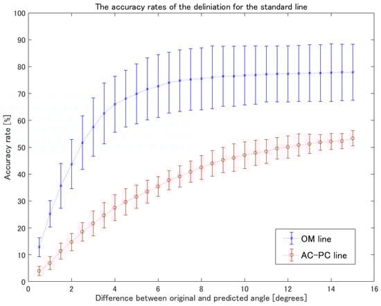
Figure 5.
The accuracy rates of delineation for the standard line. The blue asterisks indicate the mean accuracy rates of the OM-line. The red circles show the mean accuracy rates of the AC-PC line. The error bars show the standard deviation.
Table 4.
The processing speeds of calculating the standard line.
4. Discussion
This research was performed to attain detection of the specific anatomy for the delineation of two standard MRI brain lines. With regard to detecting the brain anatomies, the ROI size of 64 × 64 pixels showed a higher accuracy of detection than the 32 × 32 pixels did. This result indicates that the region including peripheral anatomies was effective for training to improve the accuracy of detection because most medical images represent the anatomy as a slice section rather than a volume. Moreover, it is not necessary to extract the anatomical structures because human anatomies are essentially all the same when no malformations are present. Since the object detection ability in self-driving cars need the ability to detect both cars and pedestrians from all directions, the required image features needed to be trained while involving the object itself, rather than the object plus its surroundings. With regard to the delineation of the standard lines for brain MRI, there were some discrepancies between the detection and accuracy rates. The delineation of the standard line was defined by two pairs of points of the Nose and Pons or the AC and PC, respectively (Appendix A). For this reason, the accuracy rates of the standard line were worse than the detection rates because the AP was different for each anatomical part. The difference of angles between the OM-line and the AC-PC line was reported as 12.6 degrees in another report [24]. In comparison, the accuracy rate of the standard line of our results showing less than 12 degrees was suggested to be adequate for the detection of the standard line for brain MRI. Since the angles of difference at 10 degrees on the OM-line and the AC-PC line between the original and predicted lines were 76.7 ± 11.0 and 47.1 ± 5.0, the delineation of the OM-line presented higher reliability for detection. The cause of the reduced accuracy rate of the AC-PC line was the lower detection accuracy on the AC because the anatomy of the AC was described as a tiny point on the sagittal image.
The limitations of the present study are as follows. First, image training was performed only using the faster R-CNN in this study. Many kinds of network models exist for object detection using deep learning. The faster R-CNN was shown to have higher mAP in several papers [6,25], which suggested that the mAP was one of the key indicators for the comparison of models. Though the weak point of the R-CNN was shown as the response speed of detections [25], the speed of response was less important during the acquisition of brain MRI. This study was not conducted to detect the dynamics of the anatomy. Second, the present study was only focusing on the deep learning technique. Though the model-based detection [20] was also one of the techniques for the detection of anatomies, the processing time of deep learning techniques has been improving [6,7,8]. We could present the processing time for the detection and delineation of the standard line within one second. However, the comparison of both techniques under the same condition should be taken into account in future research because model-based detection is also one of the robust techniques. Third, the number of training images in this study was 1200, including the images used for validation of the training. Another study [11] showed that the number of training images affected the accuracy of deep learning. Therefore, a larger number of images would improve the detection rates of the anatomy and the accuracy rates of the standard line. In this study, we focused on the detection of specific anatomical points for the delineation of the standard line of brain MRI. These results can be applied to other regions of the body and to detect tumors. The methods and results of this study will be useful for the improvement of the accuracy and will contribute to the improvement of medical image analysis, although this study focused specifically on the acquisition of brain MRI. Automatic detection for a standard line for brain MRI can help technologists improve brain MRI scans.
5. Conclusions
This study achieved the automatic detection of a standard line for brain MRI using a deep learning technique. It was found that the delineation of the standard line for brain MRI achieved a high accuracy rate on the OM-line. The use of the technique in this study can help technologists improve brain MRI examinations.
Author Contributions
H.S. proposed the idea and contributed to data acquisition, data analysis, algorithm construction, and writing and editing of the article. M.K. performed data analysis.
Funding
This research received no external funding.
Acknowledgments
The authors thank the laboratory students Shota Sato, Kazuki Narita, and Taiga Aoki for their help.
Conflicts of Interest
The authors declare that no conflicts of interest exist.
Appendix A
Figure A1 shows an example of the real time detection of the standard line for brain MRI. The software created a model for the detection of anatomies. The standard line for brain MRI was calculated in real time. This software can be also incorporated into MRI scanner consoles.

Figure A1.
Example of the real time detection of the standard line for brain MRI. The red and green dotted lines indicate the OM-line and the AC-PC line, respectively.
References
- LeCun, Y.; Bottou, L.; Bengio, Y.; Haffner, P. Gradient-Based Learning Applied to Document Recognition. Proc. IEEE 1998, 86, 2278–2324. [Google Scholar] [CrossRef]
- He, K.; Zhang, X.; Ren, S.; Sun, J. Deep Residual Learning for Image Recognition. In Proceedings of the IEEE Conference on Computer Vision and Pattern Recognition, Las Vegas, NV, USA, 27–30 June 2016; pp. 770–778. [Google Scholar]
- Krizhevsky, A.; Sutskever, I.; Hinton, G.E. Imagenet Classification with Deep Convolutional Neural Networks. In Advances in Neural Information Processing Systems; The MIT Press: Cambridge, MA, USA, 2012; pp. 1097–1105. [Google Scholar]
- Szegedy, C.; Liu, W.; Jia, Y.; Sermanet, P.; Reed, S.; Anguelov, D.; Erhan, D.; Vanhoucke, V.; Rabinovich, A. Going deeper with convolutions. In Proceedings of the IEEE Conference on Computer Vision and Pattern Recognition, Boston, MA, USA, 7–12 June 2015; pp. 1–9. [Google Scholar]
- Girshick, R.; Donahue, J.; Darrell, T.; Malik, J.; Malik, J. Rich Feature Hierarchies for Accurate Object Detection and Semantic Segmentation. In Proceedings of the IEEE Conference on Computer Vision and Pattern Recognition, Columbus, OH, USA, 23–28 June 2014; pp. 580–587. [Google Scholar]
- Liu, W.; Anguelov, D.; Erhan, D.; Szegedy, C.; Reed, S.; Fu, C.Y.; Berg, A.C. SSD: Single Shot MultiBox Detector. In European Conference on Computer Vision; Springer: Berlin/Heidelberg, Germany, 2016; pp. 21–37. [Google Scholar]
- Redmon, J.; Farhadi, A. YOLO9000: Better, Faster, Stronger. In Proceedings of the IEEE Conference on Computer Vision and Pattern Recognition (CVPR), Honolulu, HI, USA, 21–26 July 2017; pp. 6517–6525. [Google Scholar]
- Ren, S.; He, K.; Girshick, R.; Sun, J. Faster R-CNN: Towards Real-Time Object Detection with Region Proposal Networks. IEEE Trans. Pattern Anal. Mach. Intell. 2017, 39, 1137–1149. [Google Scholar] [CrossRef] [PubMed]
- Ronneberger, O.; Fischer, P.; Brox, T. U-Net: Convolutional Networks for Biomedical Image Segmentation. Exp. Algorithms 2015, 9351, 234–241. [Google Scholar]
- Sugimori, H. Evaluating the Overall Accuracy of Additional Learning and Automatic Classification System for CT Images. Appl. Sci. 2019, 9, 682. [Google Scholar] [CrossRef]
- Sugimori, H. Classification of Computed Tomography Images in Different Slice Positions Using Deep Learning. J. Health Eng. 2018, 2018, 1–9. [Google Scholar] [CrossRef] [PubMed]
- Lai, Z.; Deng, H. Medical Image Classification Based on Deep Features Extracted by Deep Model and Statistic Feature Fusion with Multilayer Perceptron. Comput. Intell. Neurosci. 2018, 2018, 1–13. [Google Scholar] [CrossRef] [PubMed]
- Yang, A.M.; Yang, X.L.; Wu, W.R.; Liu, H.X.; Zhuansun, Y.X. Research on Feature Extraction of Tumor Image Based on Convolutional Neural Network. IEEE Access 2019, 7, 24204–24213. [Google Scholar] [CrossRef]
- Masood, A.; Sheng, B.; Li, P.; Hou, X.; Wei, X.; Qin, J.; Feng, D. Computer-Assisted Decision Support System in Pulmonary Cancer detection and stage classification on CT images. J. Biomed. Inform. 2018, 79, 117–128. [Google Scholar] [CrossRef] [PubMed]
- Zhao, X.; Liu, L.; Qi, S.; Teng, Y.; Li, J.; Qian, W. Agile convolutional neural network for pulmonary nodule classification using CT images. Int. J. Comput. Assist. Radiol. Surg. 2018, 13, 585–595. [Google Scholar] [CrossRef] [PubMed]
- Gardezi, S.J.S.; Elazab, A.; Lei, B.; Wang, T. Breast Cancer Detection and Diagnosis Using Mammographic Data: Systematic Review. J. Med. Internet Res. 2019, 21, e14464. [Google Scholar] [CrossRef] [PubMed]
- Agarwal, R.; Diaz, O.; Lladó, X.; Yap, M.H.; Martí, R. Automatic mass detection in mammograms using deep convolutional neural networks. J. Med. Imaging 2019, 6, 031409. [Google Scholar] [CrossRef]
- Yeoman, L.J.; Howarth, L.; Britten, A.; Cotterill, A.; Adam, E.J. Gantry angulation in brain CT: dosage implications, effect on posterior fossa artifacts, and current international practice. Radiology 1992, 184, 113–116. [Google Scholar] [CrossRef] [PubMed]
- Talairach, J.; Tournoux, P. Co-Planar Stereotaxic Atlas of the Human Brain; Thieme Medical Publishers: New York, NY, USA, 1988; p. 122. [Google Scholar]
- Ardekani, B.A.; Bachman, A.H. Model-based Automatic Detection of the Anterior and Posterior Commissures on MRI Scans. NeuroImage 2009, 46, 677–682. [Google Scholar] [CrossRef] [PubMed]
- Mash, R.; Borghetti, B.; Pecarina, J. Improved Aircraft Recognition for Aerial Refueling Through Data Augmentation in Convolutional Neural Networks. In Proceedings of the Advances in Visual Computing: 12th International Symposium, ISVC 2016, Las Vegas, NV, USA, 12–14 December 2016; Springer: Berlin/Heidelberg, Germany, 2016; Volume 10072, pp. 113–122. [Google Scholar]
- Taylor, L.; Nitschke, G. Improving Deep Learning using Generic Data Augmentation. arXiv 2017, arXiv:170806020. [Google Scholar]
- Everingham, M.; Van Gool, L.; Williams, C.K.I.; Winn, J.; Zisserman, A. The Pascal Visual Object Classes (VOC) Challenge. Int. J. Comput. Vis. 2010, 88, 303–338. [Google Scholar] [CrossRef]
- Kim, Y.; Ahn, K.; Chung, Y.; Kim, B.-S. A New Reference Line for the Brain CT: The Tuberculum Sellae-Occipital Protuberance Line is Parallel to the Anterior/Posterior Commissure Line. Am. J. Neuroradiol. 2009, 30, 1704–1708. [Google Scholar] [CrossRef] [PubMed]
- Huang, J.; Rathod, V.; Sun, C.; Zhu, M.; Korattikara, A.; Fathi, A.; Fischer, I.; Wojna, Z.; Song, Y.; Guadarrama, S.; et al. Speed/accuracy trade-offs for modern convolutional object detectors. arXiv 2017, arXiv:161110012. [Google Scholar]
© 2019 by the authors. Licensee MDPI, Basel, Switzerland. This article is an open access article distributed under the terms and conditions of the Creative Commons Attribution (CC BY) license (http://creativecommons.org/licenses/by/4.0/).