Development of Path Planning Tool for Unmanned System Considering Energy Consumption


Abstract
:1. Introduction
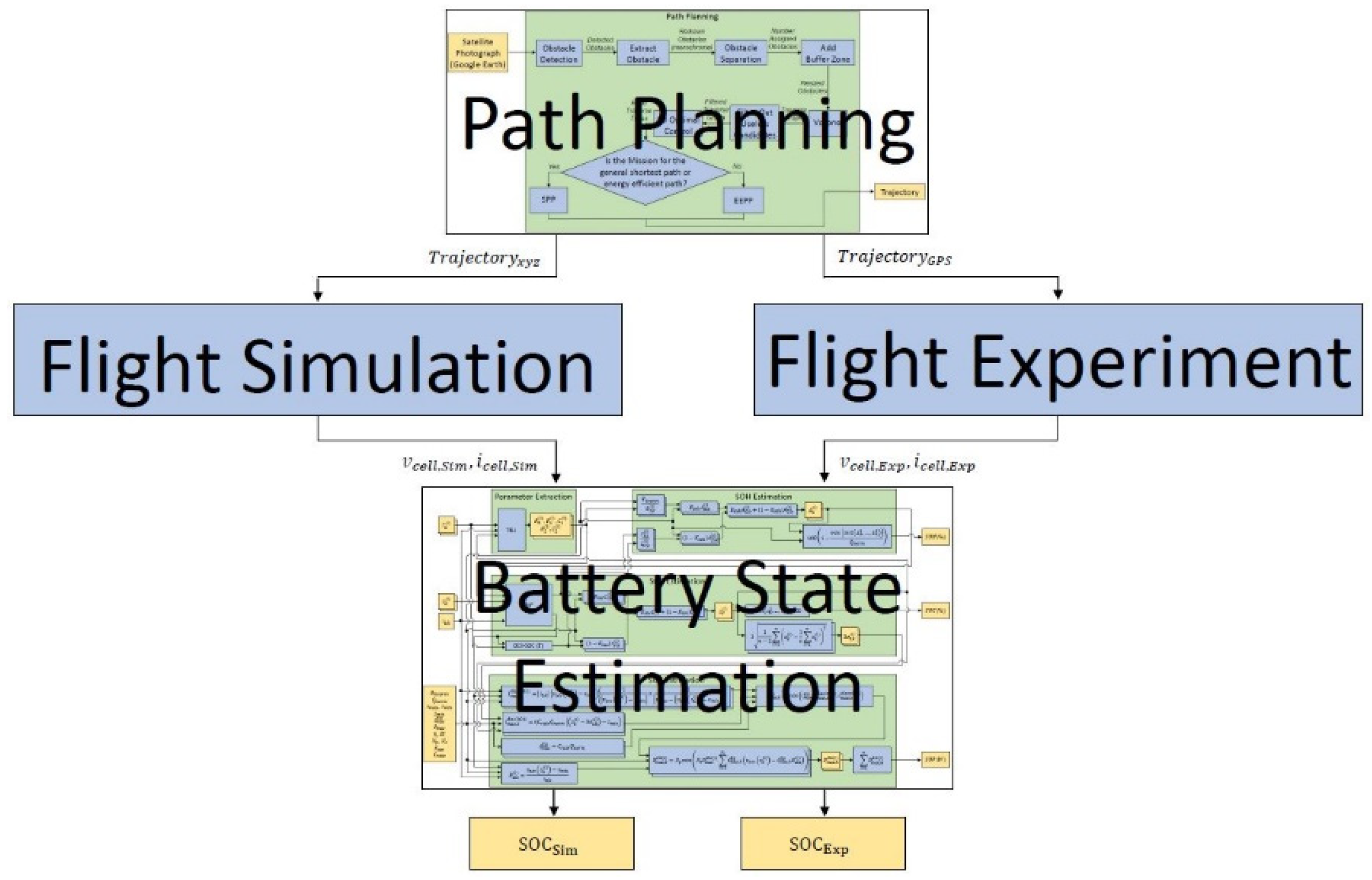
2. Mission Hierarchy
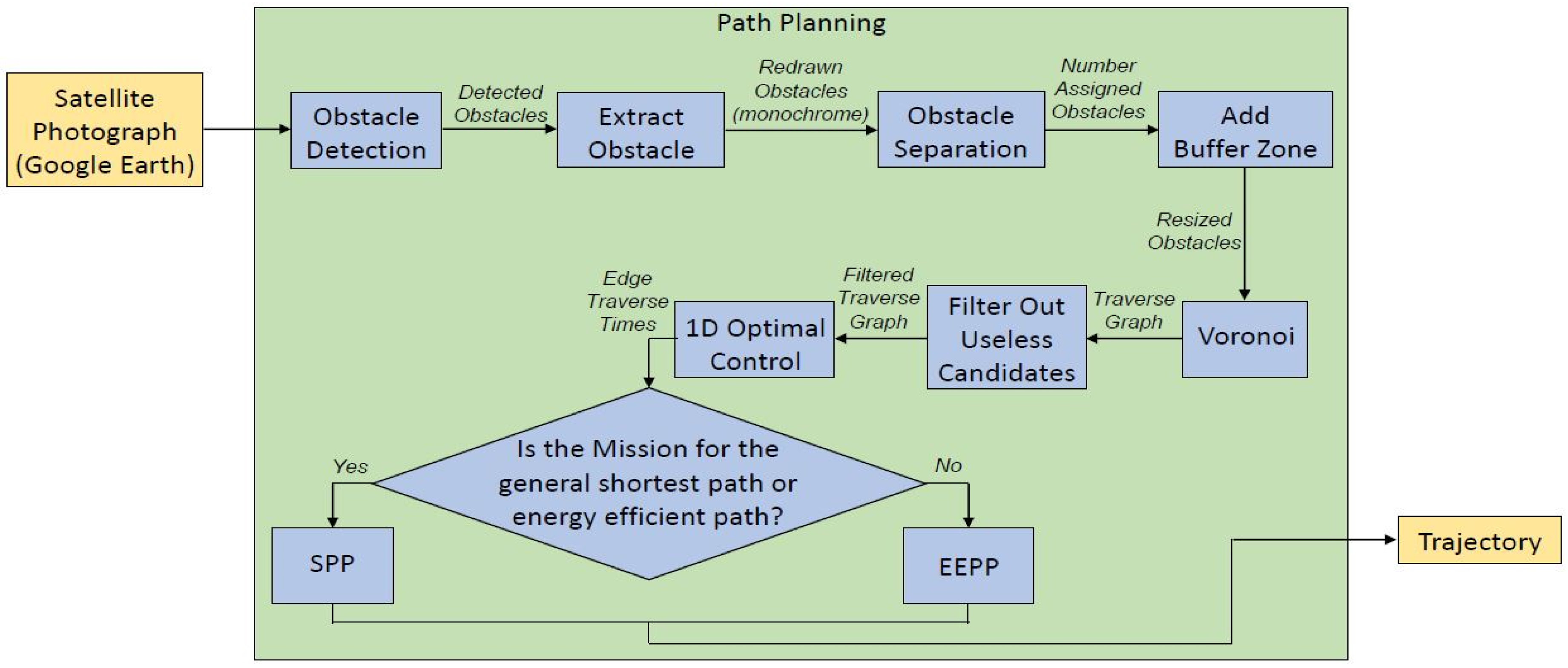
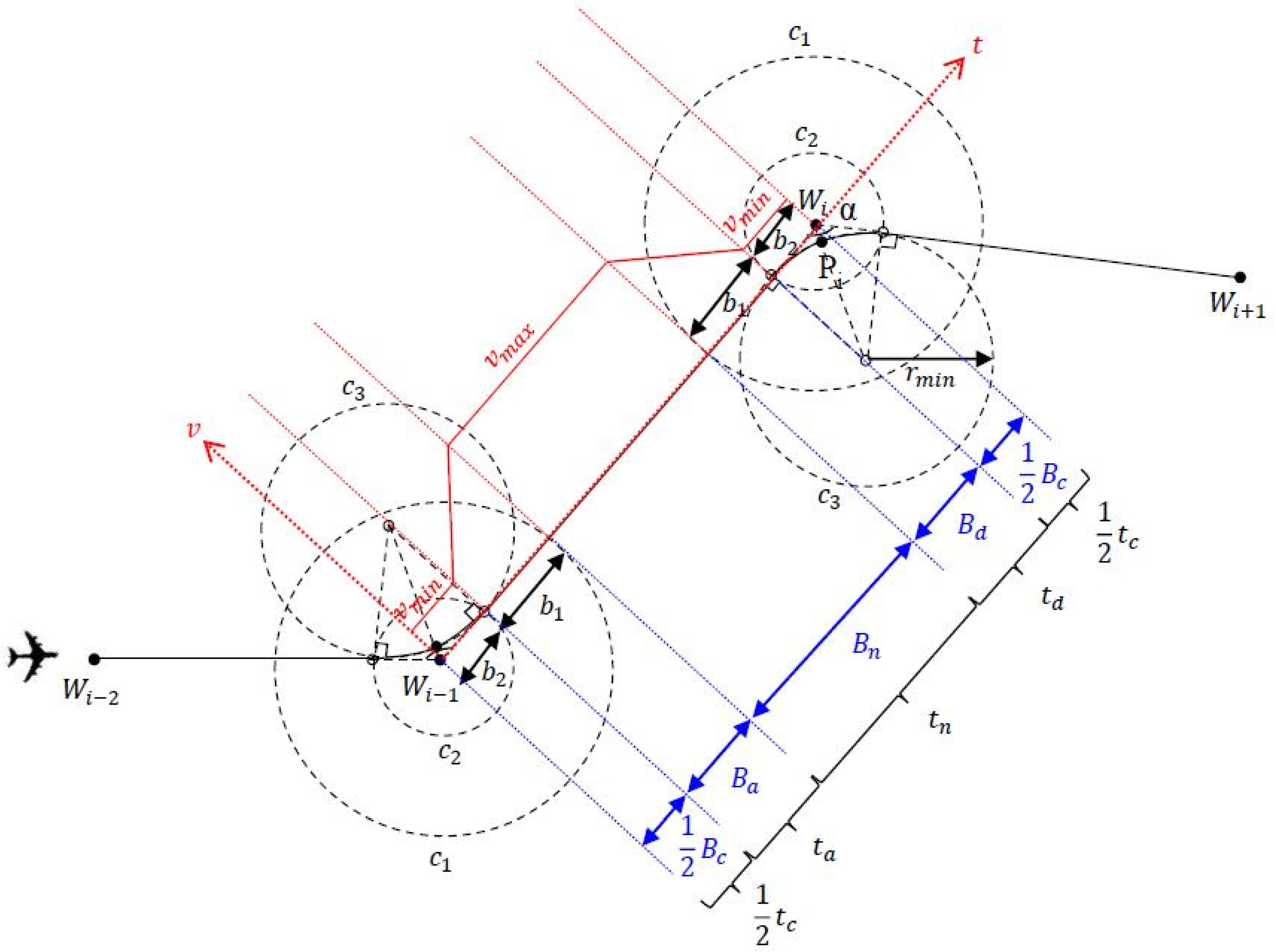
3. Path Planning
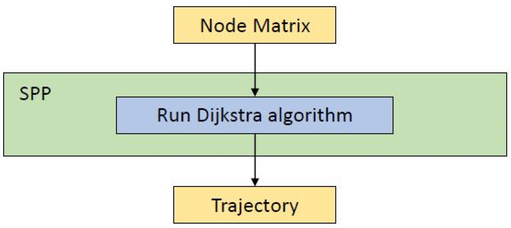
3.1. SPP
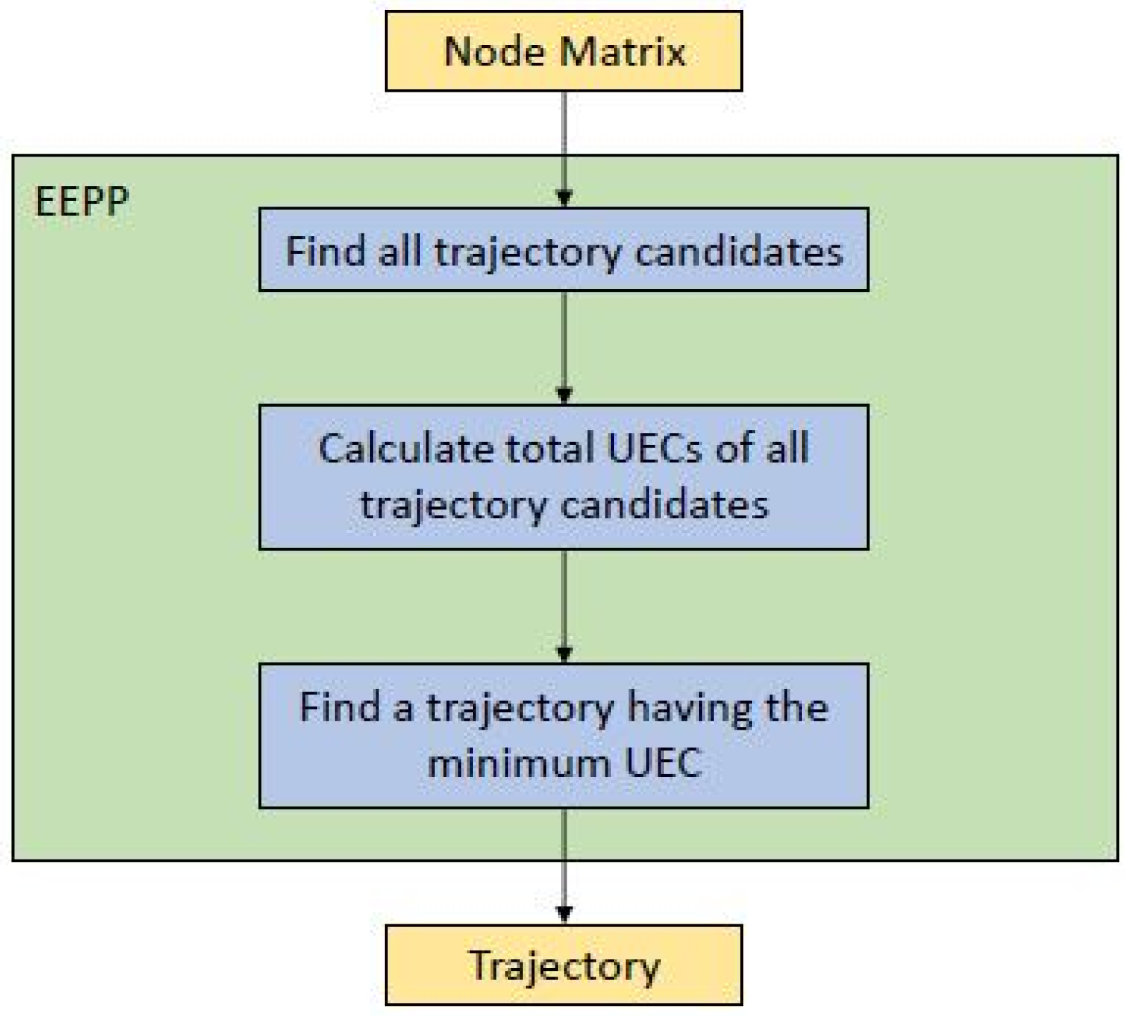
3.2. EEPP
4. Mathematical Modeling of the UAV and Battery Pack
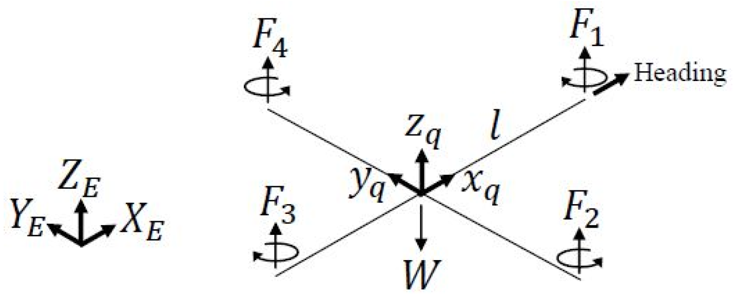
4.1. UAV
4.2. Battery Pack
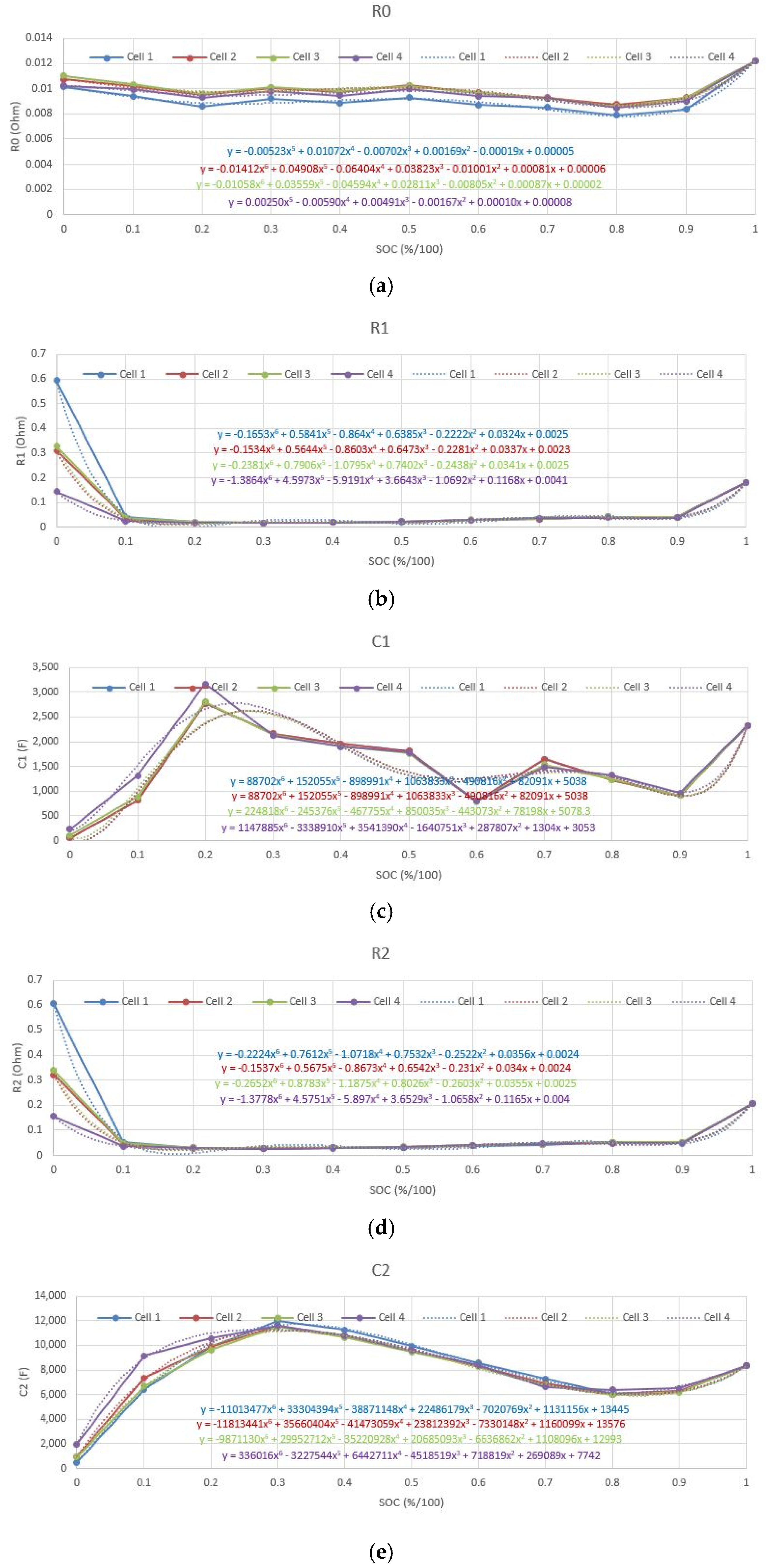
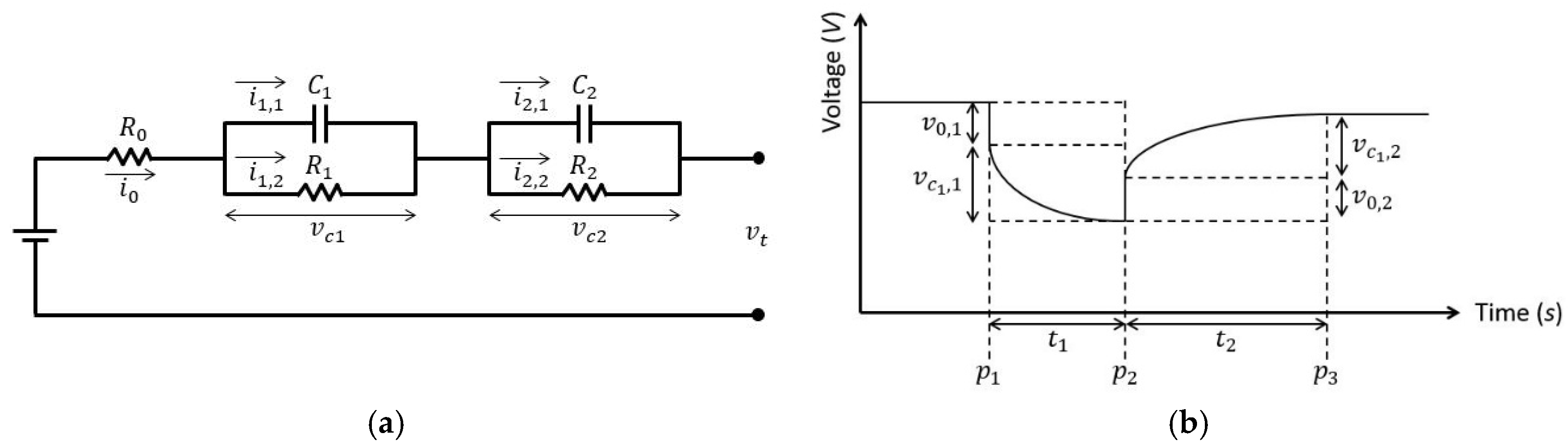
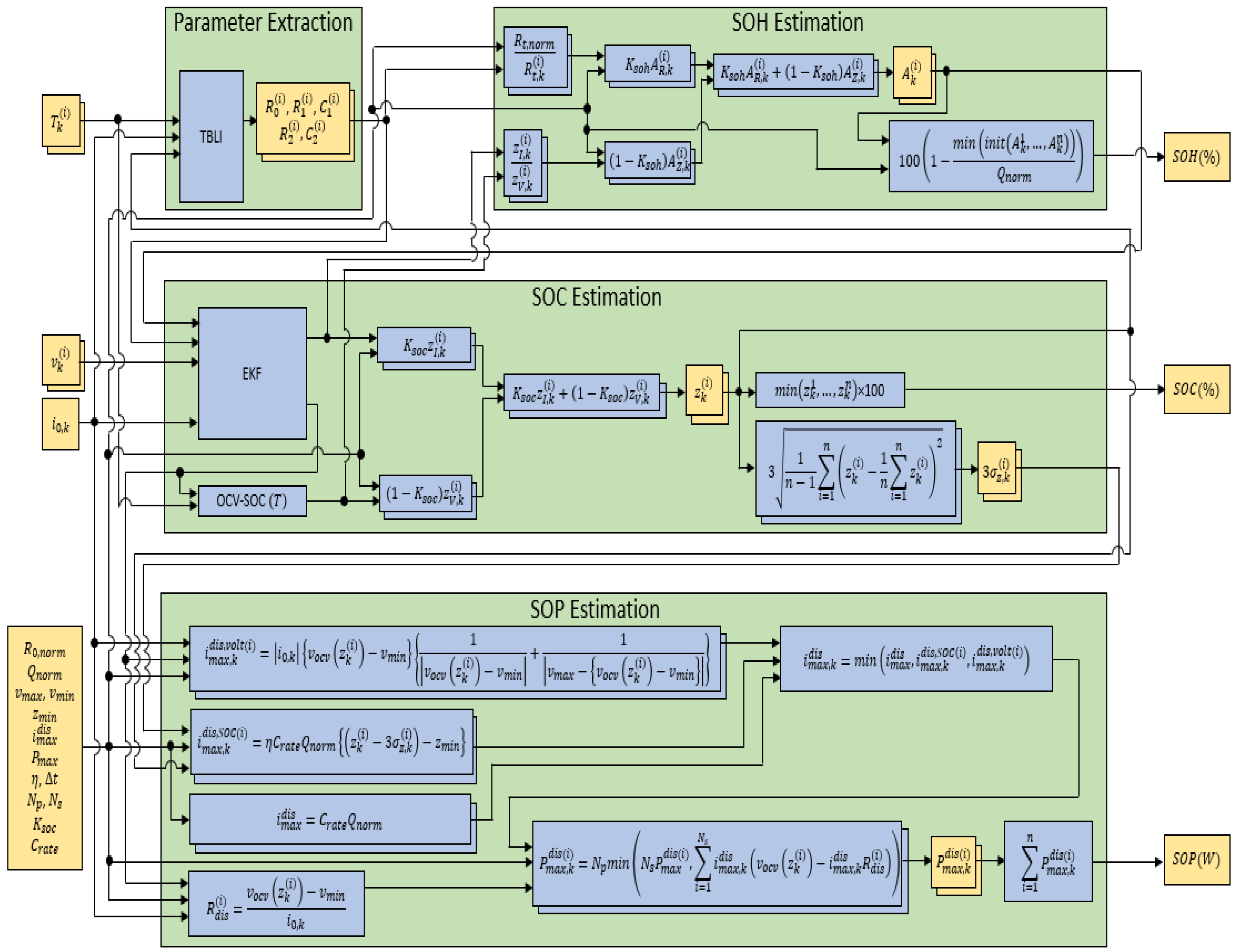
4.2.1. ECM
4.2.2. TBLI Parameter Identification
4.2.3. SOC and SOP State Estimation
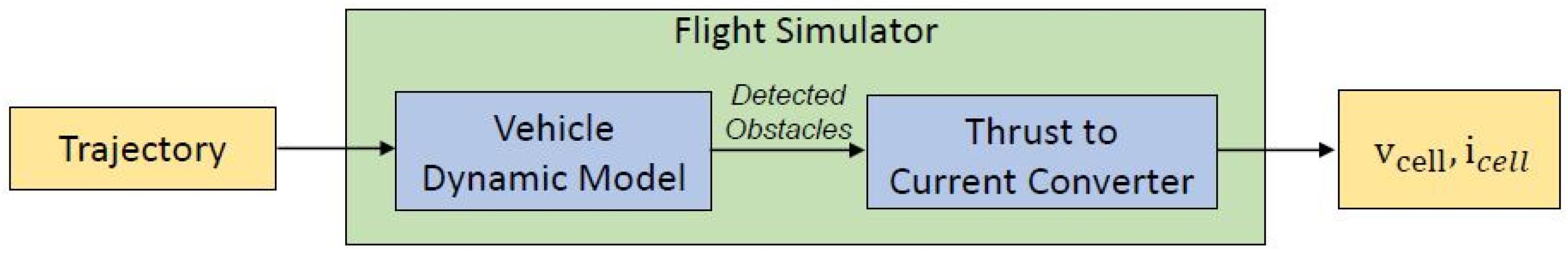
5. Simulation and Experimental Setups
5.1. Simulation Setup
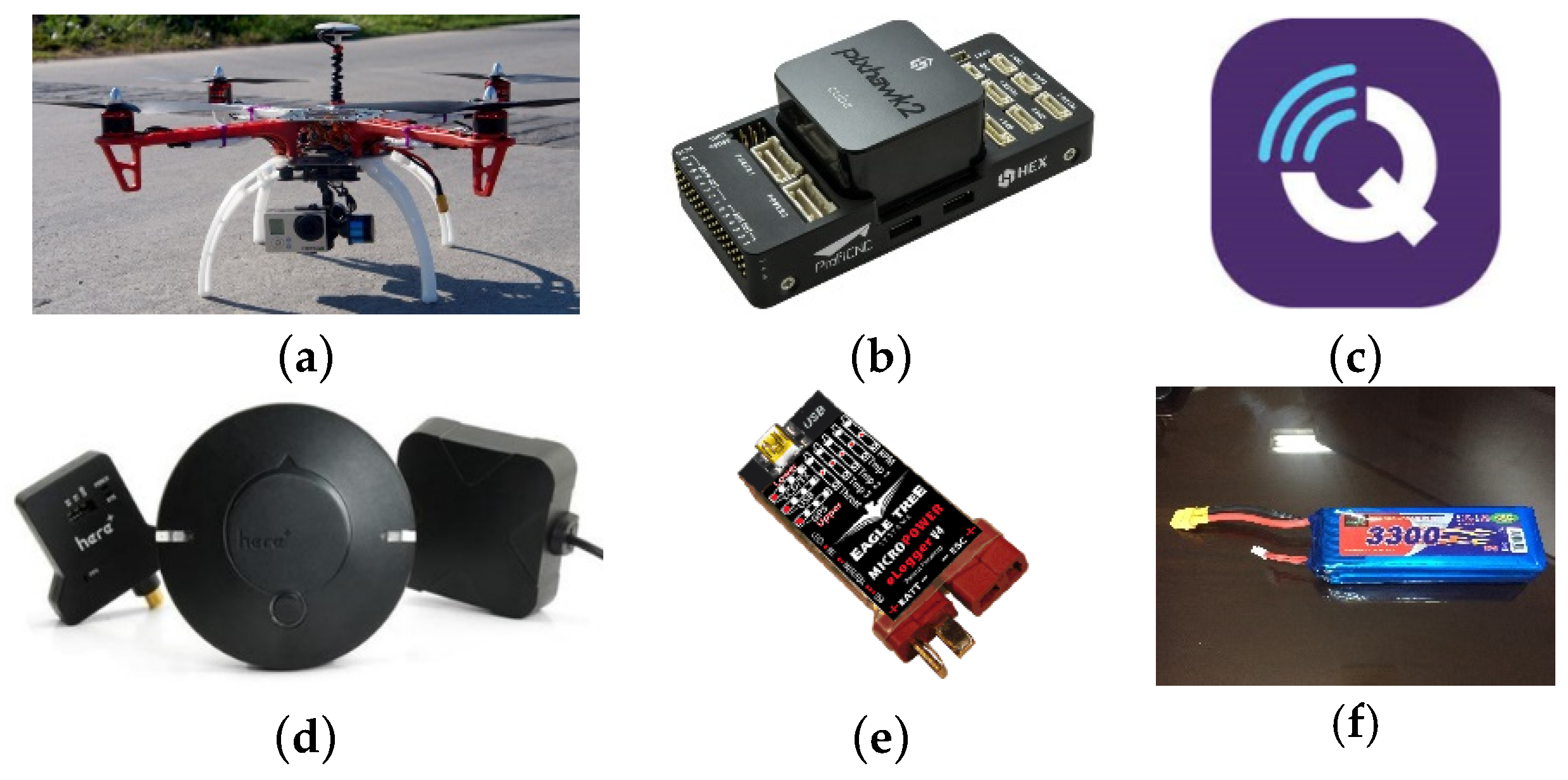
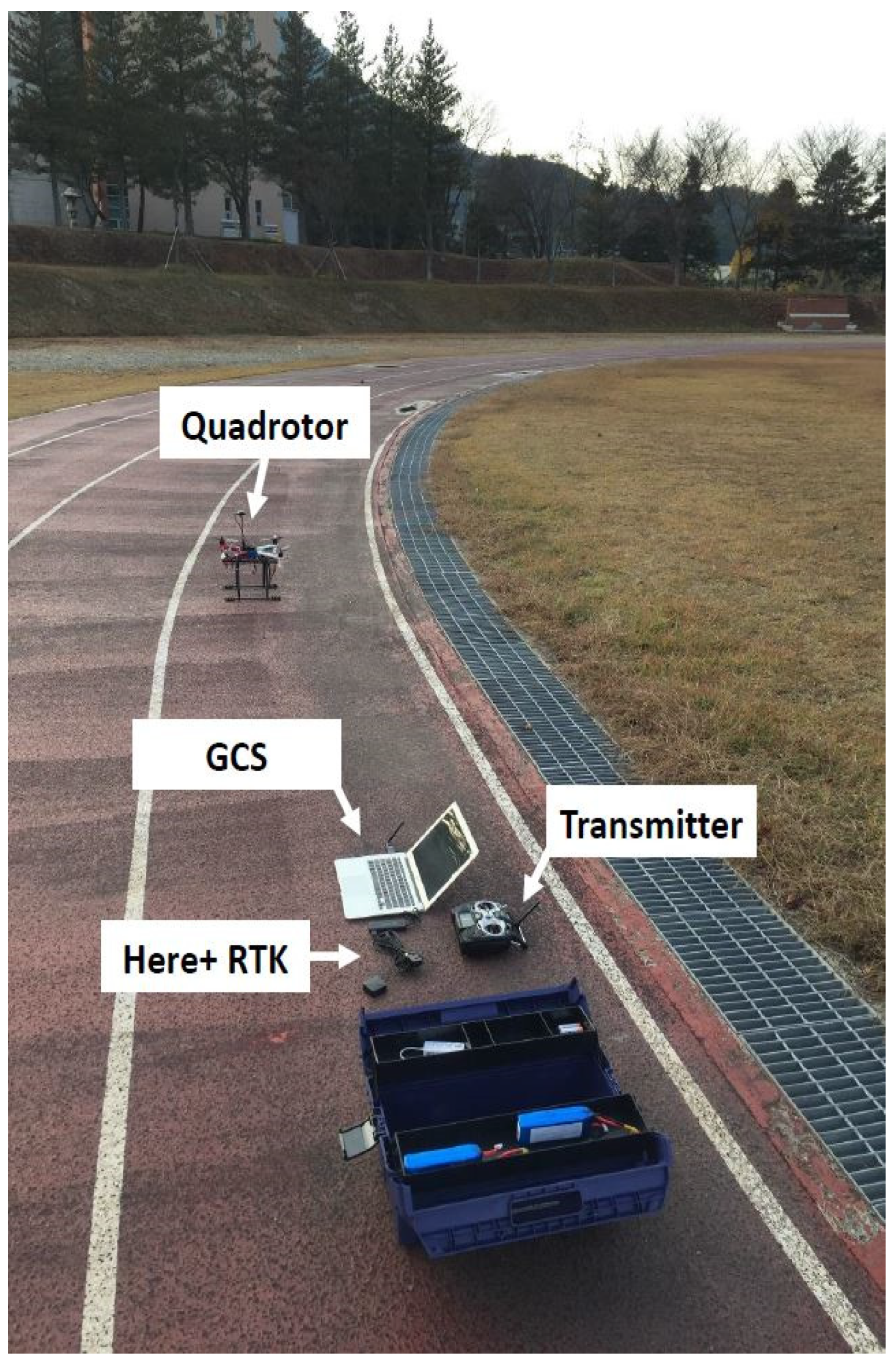
5.2. Experiment Setup
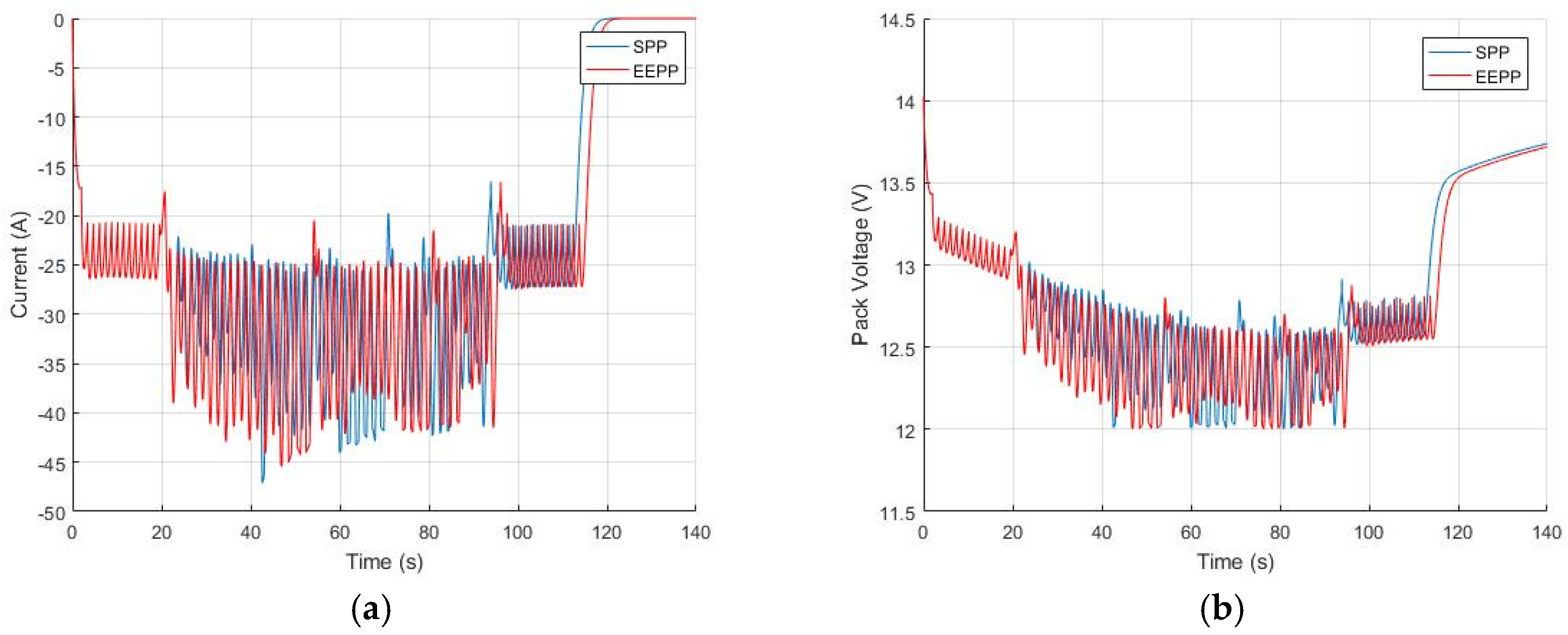
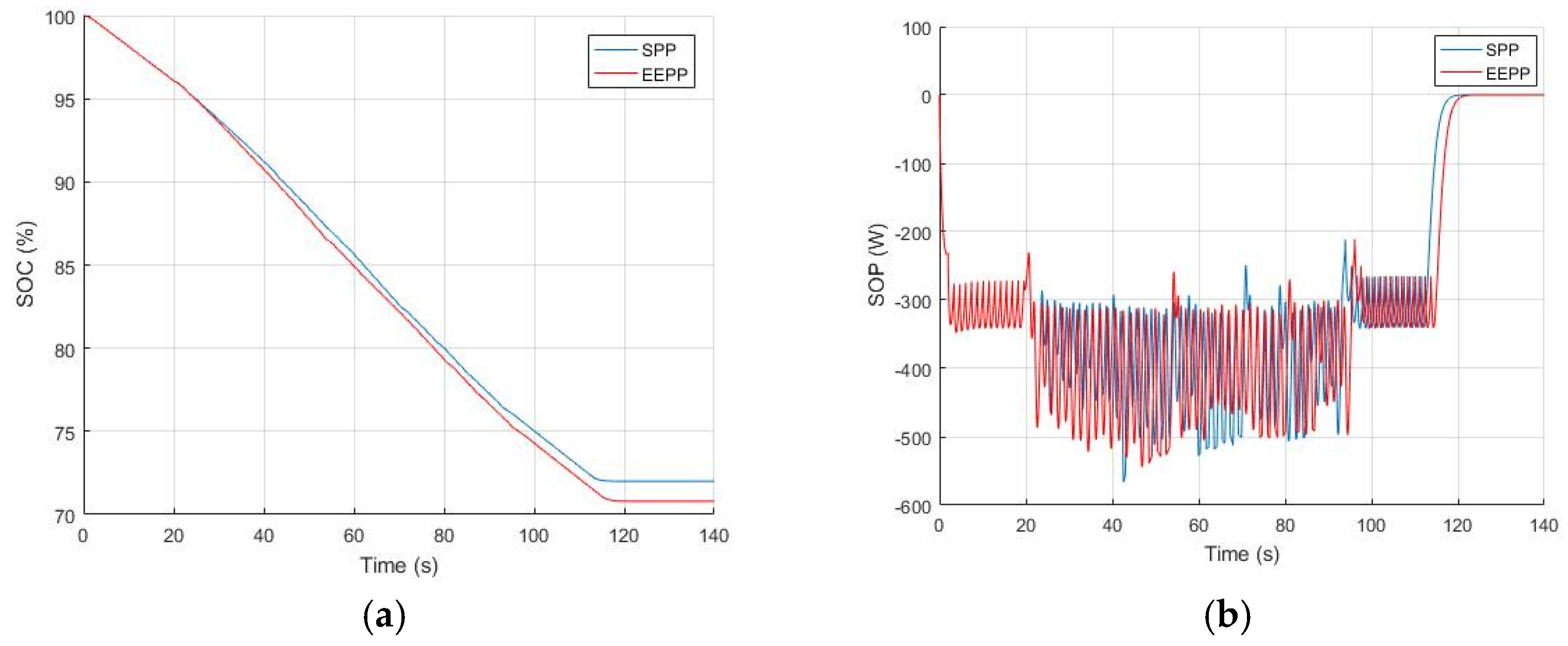
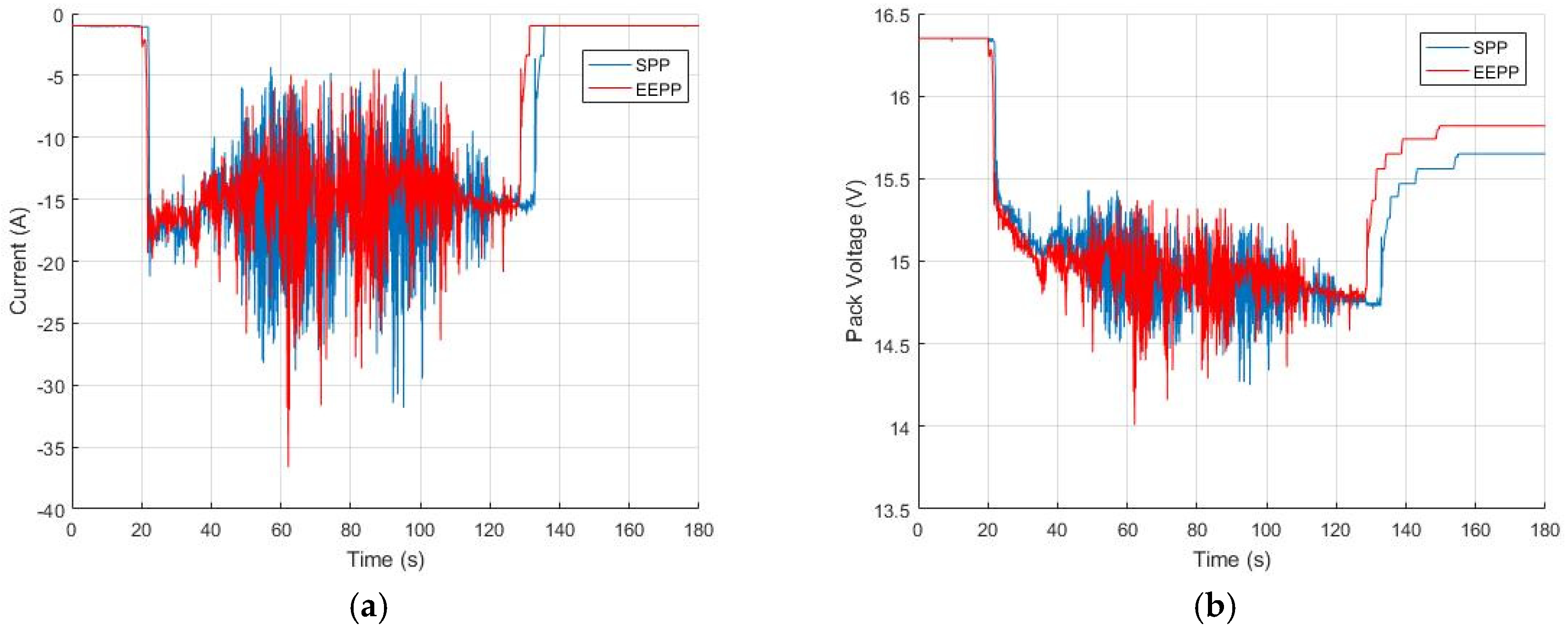
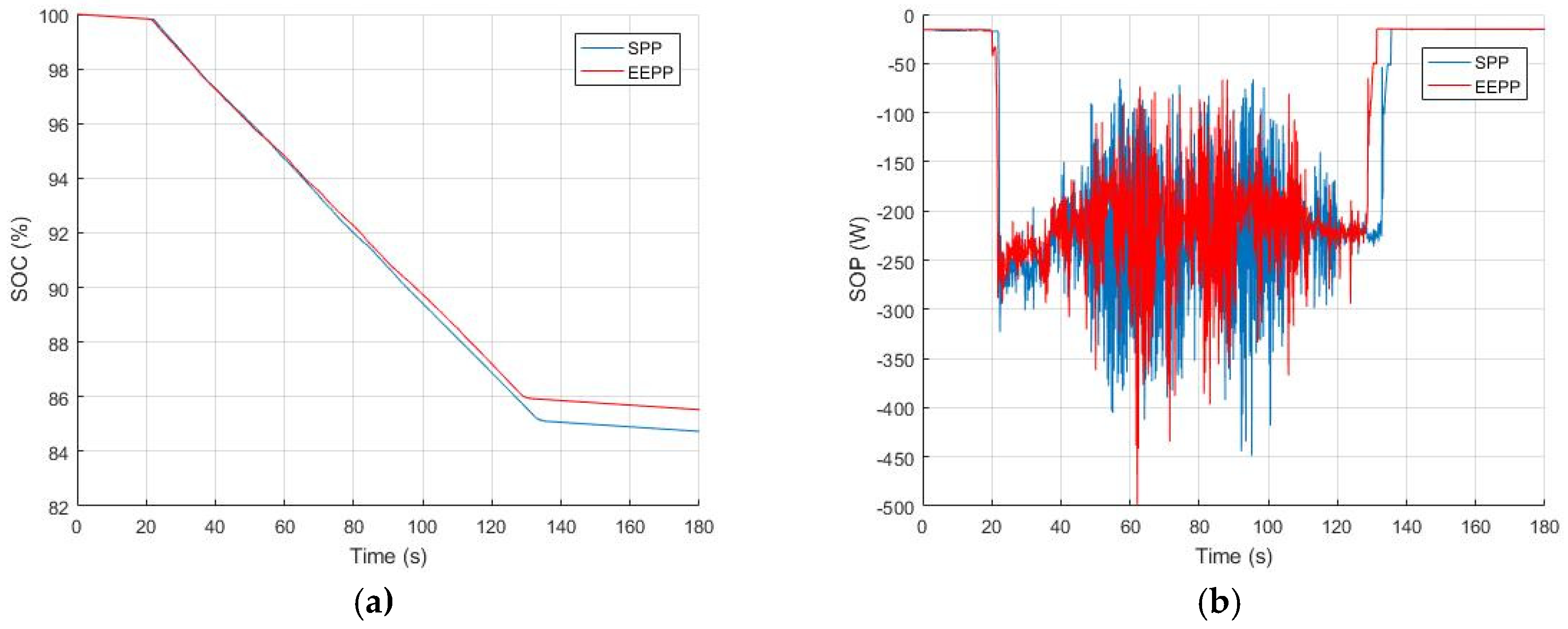
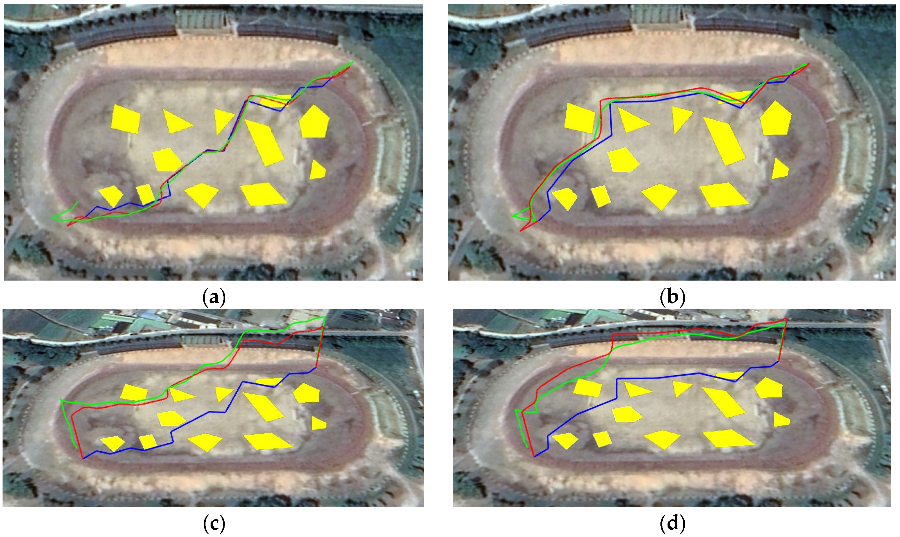
6. Simulation and Experimental Results
6.1. Simulation Result
6.2. Experimental Result
7. Conclusions
Acknowledgments
Conflicts of Interest
Appendix A
Appendix B
References
- Kim, K.; Kim, T.; Lee, K.; Kwon, S. Fuel Cell System with Sodium Borohydride as Hydrogen Source for Unmanned Aerial Vehicles. J. Power Sources 2011, 196, 9069–9075. [Google Scholar] [CrossRef]
- Gao, X.; Hou, Z.; Guo, Z.; Fan, R.; Chen, X. The Equivalence of Gravitational Potential and Rechargeable Battery for High-Altitude Long-Endurance Solar-Powered Aircraft on Energy Storage. Energy Convers. Manag. 2013, 76, 986–995. [Google Scholar] [CrossRef]
- Khaligh, A.; Li, Z. Battery, Ultracapacitor, Fuel Cell, and Hybrid Energy Storage Systems for Electric, Hybrid Electric, Fuel Cell, and Plug-In Hybrid Electric Vehicles: State of the Art. IEEE Trans. Veh. Technol. 2010, 59, 2806–2814. [Google Scholar] [CrossRef]
- Noorden, R.A. Better Battery—Chemists are Reinventing Rechargeable Cells to Drive Down Costs and Boost Capacity. Nature 2014, 507, 26–28. [Google Scholar] [PubMed]
- Chang, Y.S.; Lee, H.J. Optimal Delivery Routing with Wider Drone-Delivery Areas Along a Shorter Truck-Route. Expert Syst. Appl. 2018, 104, 307–317. [Google Scholar] [CrossRef]
- Rubio, J.C.; Vagners, J.; Rysdyk, R. Adaptive Path Planning for Autonomous UAV Oceanic Search Missions. In Proceedings of the AIAA 1st Intelligent Systems Technical Conference, Chicago, IL, USA, 20–22 September 2004. [Google Scholar]
- Oliva, J.A.; Weihrauch, C.; Bertram, T. A Model-Based Approach for Predicting the Remaining Driving Range in Electric Vehicles. In Proceedings of the Annual Conference of the Prognostics and Health Management Society, New Orleans, LA, USA, 14–17 October 2013. [Google Scholar]
- Ondruska, P.; Posner, I. Probabilistic Attainability Maps: Efficiently Predicting Driver-Specific Electric Vehicle Range. In Proceedings of the IEEE Intelligent Vehicles Symposium Proceedings, Dearborn, MI, USA, 8–11 June 2014. [Google Scholar]
- Ferreira, J.C.; Monteiro, V.; Afonso, J.L. Dynamic Range Prediction for an Electric Vehicle. In Proceedings of the EVS27 International Battery, Hybrid and Fuel Cell Electric Vehicle Symposium, Barcelona, Spain, 17–20 November 2013. [Google Scholar]
- Plett, G.L. Battery Management Systems, II: Equivalent-Circuit Methods, 2nd ed.; Artech House Publishers: Norwood, MA, USA, 2014. [Google Scholar]
- Sharma, O.P. Analysis and Parameter Estimation of Li-Ion Batteries Simulations for Electric Vehicles. In Proceedings of the American Control Conference, San Francisco, CA, USA, 29 June–21 July 2011. [Google Scholar]
- Thanagasundram, S.; Arunachala, R.; Makinejad, K.; Teutsch, T.; Jossen, A. A Cell Level Model for Battery Simulation. In Proceedings of the European Electric Vehicle Congress, Brussels, Belgium, 20–22 November 2012. [Google Scholar]
- Plett, G.L. Extended Kalman Filtering for Battery Management Systems of LiPB-based HEV Battery Packs–Part 3. State and Parameter Estimation. J. Power Sources 2004, 134, 277–292. [Google Scholar] [CrossRef]
- Jung, S.; Ariyur, K.B. Robustness for Scalable Autonomous UAV Operations. Int. J. Aeronaut. Space Sci. 2017, 18, 767–779. [Google Scholar] [CrossRef]
- Jung, S.; Ariyur, K.B. Scalable Autonomy for UAVs. In Proceedings of the AIAA Infotech@Aerospace, St. Louis, MO, USA, 29–31 March 2011. [Google Scholar]
- Leishman, J.G. Principles of Helicopter Aerodynamics, 2nd ed.; Cambridge University Press: Cambridge, UK, 2002. [Google Scholar]
- Dorling, K.; Heinrichs, J.; Messier, G.G.; Magierowski, S. Vehicle Routing Problems for Drone Delivery. IEEE Trans. Syst. Man Cybern. Syst. 2017, 47, 70–85. [Google Scholar] [CrossRef]
- Dubins, L.E. On Curves of Minimal Length with a Constraint on Average Curvature and with Prescribed Initial and Terminal Positions and Tangent. Am. J. Math. 1957, 79, 497–516. [Google Scholar] [CrossRef]
- Tsourdos, A.; White, B.; Shanmugavel, M. Cooperative Path Planning of Unmanned Aerial Vehicles, 1st ed.; John Wiley & Sons: Chichester, UK, 2011. [Google Scholar]
- Jung, S.; Ariyur, K.B. Enabling Operational Autonomy for UAVs with Scalability. AIAA J. Aerosp. Inf. Syst. 2013, 10, 516–529. [Google Scholar]
- Robotics, P.C. Vision and Control: Fundamental Algorithms in MATLAB; Springer: Berlin/Heidelberg, Germany, 2011. [Google Scholar]
- Jung, S.; Ariyur, K.B. Strategic Cattle Roundup using Multiple Quadrotor UAVs. Int. J. Aeronaut. Space Sci. 2017, 18, 315–326. [Google Scholar] [CrossRef]
- Jung, S.; Jeong, H. Extended Kalman Filter-Based State of Charge and State of Power Estimation Algorithm for Unmanned Aerial Vehicle Li-Po Battery Pack. Energies 2017, 10, 1237. [Google Scholar] [CrossRef]
- Steven, B.L.; Lewis, F.L. Aircraft Control and Simulation; John Wiley & Sons: New York, NY, USA, 2003. [Google Scholar]
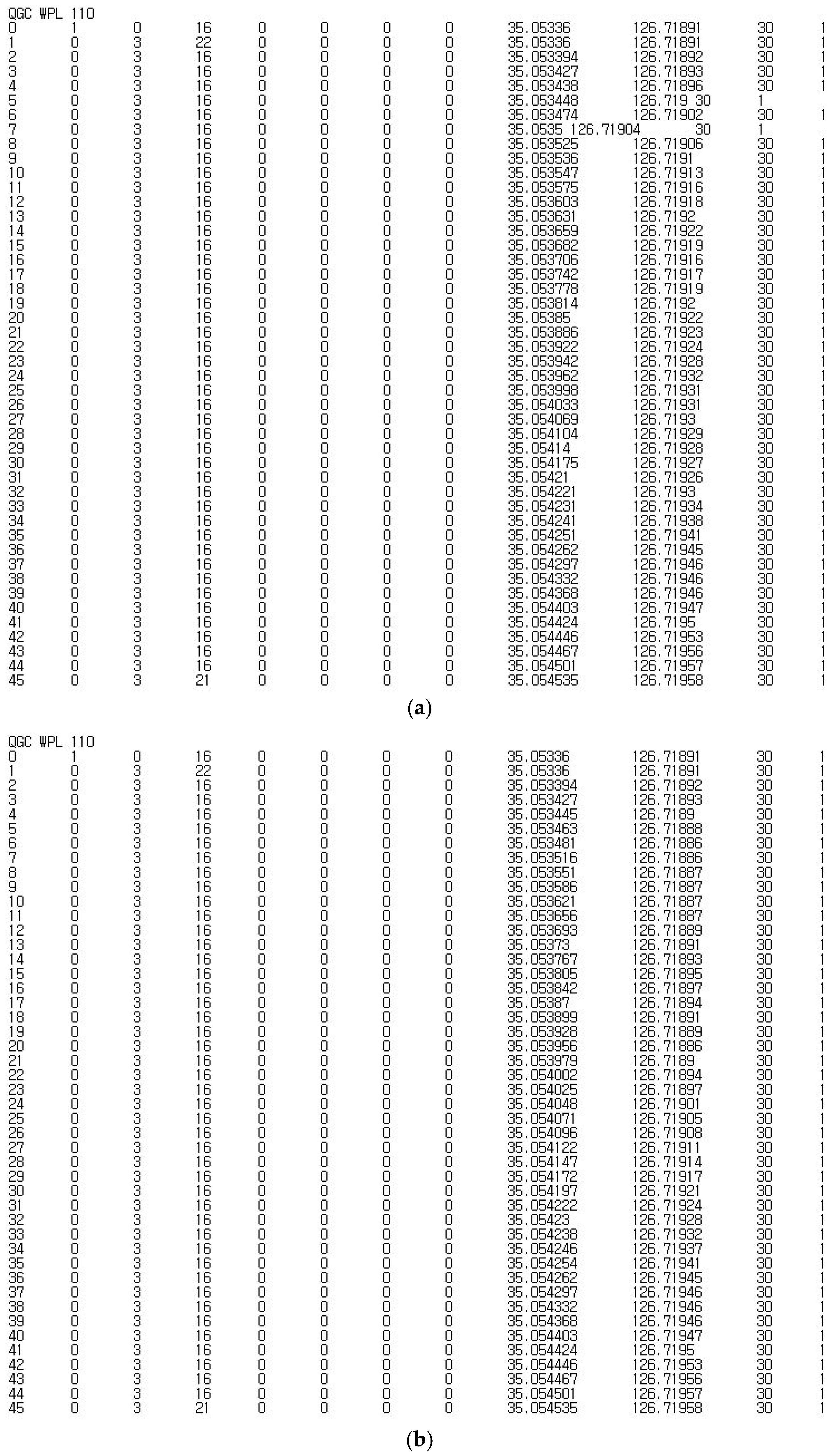
- QGroundControl—Waypoint Protocol. Available online: https://goo.gl/SqVVzd (accessed on 28 June 2018).

| QGC WPL < VERSION> | |||||
|---|---|---|---|---|---|
| <INDEX> | <CURRENT WP> | <COORD FRAME> | <COMMAND> | <PARAM1> | <PARAM2> |
| <PARAM3> | <PARAM4> | <PARAM5/X/ | < PARAM6/Y/ | < PARAM5/Z/ | <AUTOCONTINUE> |
| LONGITUDE> | LATITUDE > | ALTITUDE > | |||
| SPP | EEPP | |||
|---|---|---|---|---|
| Prediction Value | Actual Value | Prediction Value | Actual Value | |
| Total Trajectory Distance () | 204.63 | 193.30 | 208.76 | 201.08 |
| Min Speed of UAV () | 0 | 0 | 0 | 0 |
| Max Speed of UAV () | 5 | 0.34 | 5 | 0.33 |
| Weight of UAV () | 1.41 | 1.41 | 1.41 | 1.41 |
| Total UEC () | 4.47 | 11.54 | 5.71 | 11.99 |
| Algorithm Run Time () | 11.51 | 20.34 | ||
| SOC Leftover () | 72.00 | 70.80 | ||
| SOP Peak () | 566.20 | 543.47 | ||
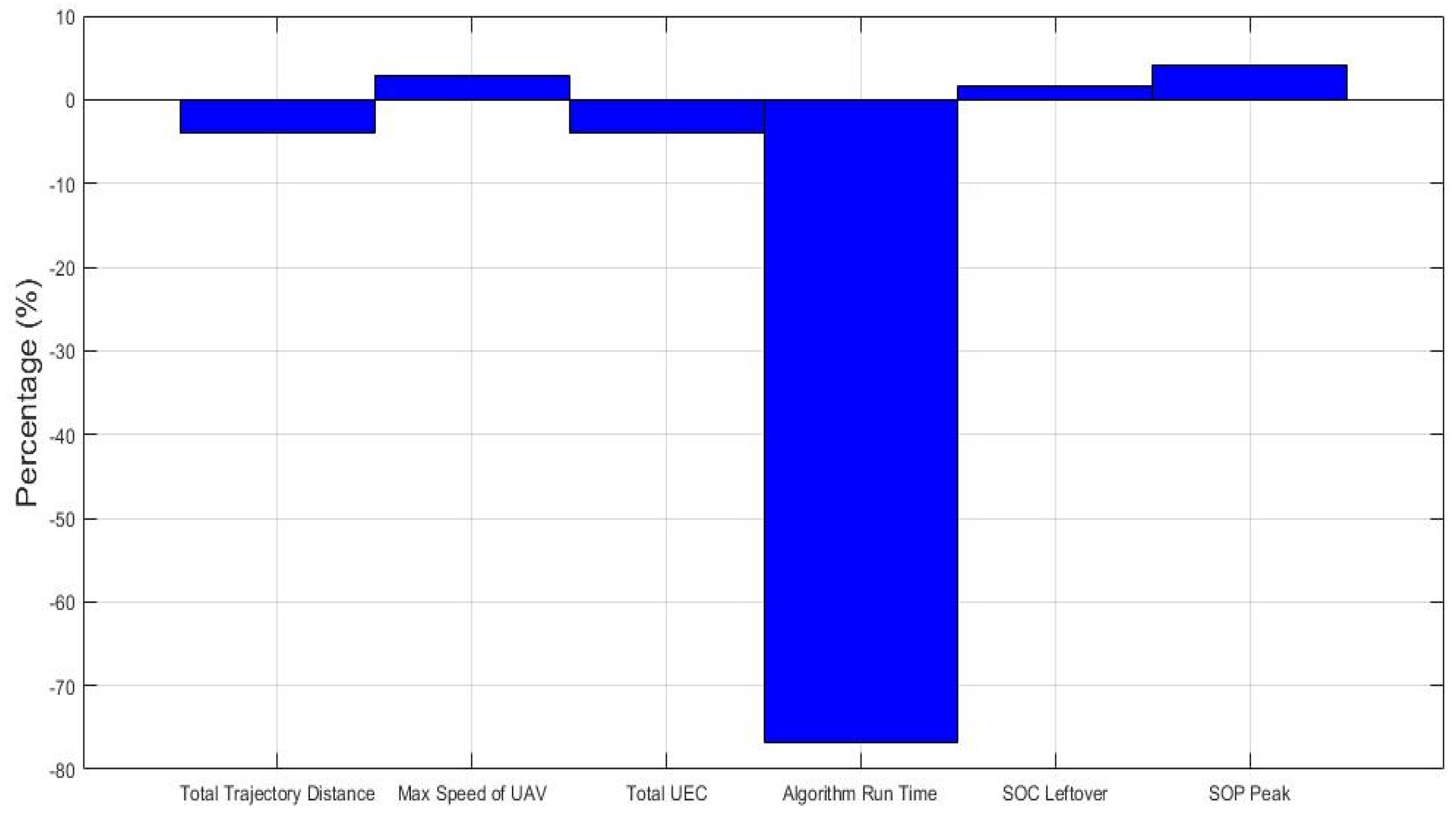
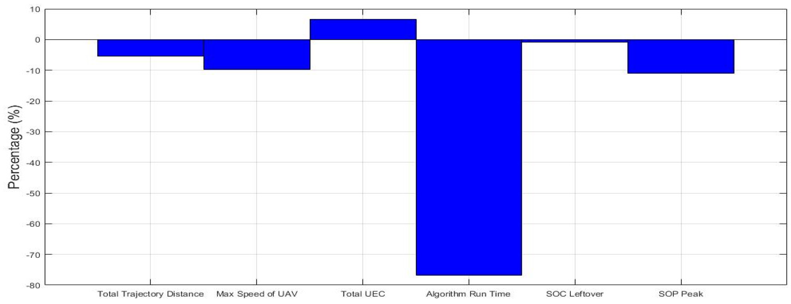
| Total Trajectory Distance () | −4.02 |
| Min. Speed of UAV () | 0 |
| Max. Speed of UAV () | 2.94 |
| Weight of UAV () | 0 |
| Total UEC () | −3.90 |
| Algorithm Run Time () | −76.72 |
| SOC Leftover () | 1.67 |
| SOP Peak () | 4.01 |
| SPP | EEPP | |||
|---|---|---|---|---|
| Prediction Value | Actual Value | Prediction Value | Actual Value | |
| Total Trajectory Distance () | 205.75 | 174.11 | 212.17 | 183.64 |
| Min. Speed of UAV () | 0 | 0 | 0 | 0 |
| Max. Speed of UAV () | 5 | 4.20 | 5 | 4.61 |
| Weight of UAV () | 1.41 | 1.41 | 1.41 | 1.41 |
| Total UEC () | 4.47 | 7.94 | 5.71 | 7.41 |
| Algorithm Run Time () | 11.51 | 20.34 | ||
| SOC Leftover () | 83.73 | 84.53 | ||
| SOP Peak () | 448.85 | 498.37 | ||
| Total Trajectory Distance () | −5.47 |
| Min. Speed of UAV () | 0 |
| Max. Speed of UAV () | −9.76 |
| Weight of UAV () | 0 |
| Total UEC () | 6.68 |
| Algorithm Run Time () | −76.72 |
| SOC Leftover () | −0.96 |
| SOP Peak () | −11.03 |
© 2019 by the author. Licensee MDPI, Basel, Switzerland. This article is an open access article distributed under the terms and conditions of the Creative Commons Attribution (CC BY) license (http://creativecommons.org/licenses/by/4.0/).
Share and Cite
Jung, S. Development of Path Planning Tool for Unmanned System Considering Energy Consumption. Appl. Sci. 2019, 9, 3341. https://doi.org/10.3390/app9163341
Jung S. Development of Path Planning Tool for Unmanned System Considering Energy Consumption. Applied Sciences. 2019; 9(16):3341. https://doi.org/10.3390/app9163341
Chicago/Turabian StyleJung, Sunghun. 2019. "Development of Path Planning Tool for Unmanned System Considering Energy Consumption" Applied Sciences 9, no. 16: 3341. https://doi.org/10.3390/app9163341
APA StyleJung, S. (2019). Development of Path Planning Tool for Unmanned System Considering Energy Consumption. Applied Sciences, 9(16), 3341. https://doi.org/10.3390/app9163341