Procedural Method for Fast Table Mountains Modelling in Virtual Environments

Featured Application

The presented approach can be implemented as an interactive tool for creating mesa and butte terrain features in modelling applications and game engines.

Abstract

Natural terrains created by long-term erosion processes can sometimes have spectacular forms and shapes. The visible form depends often upon internal geological structure and materials. One of the unique terrain artefacts occur in the form of table mountains and can be observed in the Monument Valley (Colorado Plateau, USA). In the following article a procedural method is considered for terrain modelling of structures, geometrically similar to the mesas and buttes hills. This method is not intended to simulate physically inspired erosion processes, but targets directly the generation of eroded forms. The results can be used as assets by artists and designers. The proposed terrain model is based on a height-field representation extended by materials and its hardness information. The starting point of the technique is the Poisson Faulting algorithm that was originally used to obtain fractional Brownian surfaces. In the modification, the step function as the fault line generator was replaced with a circular one. The obtained geometry was used for materials’ classification and the hardness part of the modelled terrain. The final model was achieved by the erosive modification of geometry according to the materials and its hardness data. The results are similar to the structures observed in nature and are achieved within an acceptable time for real-time interactions.

1. Introduction

The terrain model is a very important asset in open world virtual environments, e.g., military training systems or video games [1,2,3,4]. It is responsible for getting an accurate impression of the appropriate scale and proportion of other objects placed in the scene. A more accurate synthetic terrain increases the visual acceptability of the virtual environment and leads to better immersion. Thus, models of natural landscapes should depict the impact of erosion forces on terrain structures [5,6,7].

The importance of the internal structure in terrain modelling was under consideration in related research [8,9,10] and addressed especially in the physically-inspired simulation of the hydraulic erosion [11,12] and geology driven method [13]. Materials’ distributions are also important in the modelling of table mountains. The topic was previously discussed by Beneš and Arriaga [14] in a simulation-based method. In their technique, the terrain was composed from two different materials. The hard material (rock) eroded to the soft one (sand) due to exposure to an environmental condition. The soft material was transported down by gravity-driven diffusion and deposited at the model base.

Data structures for terrain models can be categorised into two main types, however, both of them have weaknesses and advantages. The matrices of elevation values i.e., height fields are the simplest and most commonly used for terrain models. This is due to the ease of implementation of procedural methods for generating and rendering synthetic landforms [9,15,16,17,18]. The main disadvantage of this representation is the inability to replicate models with aspherical topology [19]. Complex models are based on volumetric representation. In this case, all techniques are much more complicated, but it is possible to achieve landforms unreachable in height-based structures (also in aspherical topology) e.g., caves, rock shelves, or arches [13,14,17]. Hybrid methods can be also isolated by trying to cumulate positive aspects of both main representations, while minimising their weaknesses. Beneš and Forsbach introduced layered representation consisting of stacked horizontal materials, where each has its own elevation and geological attributes [8,15,16,18].

Since the works of Mandelbrot, fractal geometry plays an important role in computer-assisted terrain modelling [18,20,21,22]. Fractal based terrains range from the basic self-similar, noise-based structures to more naturally eroded landforms expanded by rivers and coastlines [9,10,23,24,25,26,27,28]. Further research into landscape synthesis was inspired by natural phenomena, especially erosion and their new directions. Modern modelling techniques are inspired by hydrology [7,29,30,31,32], geology [13,33], genetic programming [34], patch and feature identification [35], hierarchical models [36], shape grammar [37], or particle systems [38,39]. Another interesting approach to terrain modelling is to synthesise complete landscapes by machine learning procedures. The methods are user oriented and provide tools for modelling with few simple starting rules [5].

In this article, a procedural technique is proposed for the generation of buttes and mesas terrain formations. The method is not intended to simulate dynamic, complex, and time-consuming erosive processes, but the effects they cause is directed for artist and designers, so as to quickly provide assets for further use. In the proposed solution, a terrain model is layered [8], represented by classic height-field [15,16,18] extended by information about distribution and hardness of the materials. The method is based on fractal geometry [22] and modified by the Poisson Faulting algorithm [40], whereby the geometry layer is obtained. On this basis, the material classification is performed and stored in the materials’ layer. This layer also provides information on the materials’ distribution. Next, the hardness layer is filled with desired data [41]. After model preparation, the erosive procedure is performed, consisting of geometric gradation and soil levelling. It is worth emphasising that in contrast to dynamic simulations-based methods, the paper focuses on achieving “on the fly” eroded structures without time-consuming processes. The presented approach concentrates on the preparation of terrain assets representing a range of table structures. The implementation works fast and can be used in interactive frameworks. The general schema of the procedure, including preparation of an initial model and erosion section is shown in Figure 1.

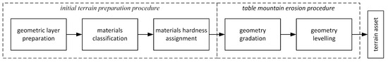
Figure 1. General schema of the proposed method.

The paper is organised as follows. In Section 2, the new approach that allows the generation of a new terrain model is proposed. Section 3 contains the method for the simulation of the table mountain erosion process. Section 4 is devoted to results obtained with the application of the proposed approach. Finally, the last section concludes the paper.

2. Terrain Model

Table mountains are a spectacular natural terrain formation, usually found in the form of isolated hills knows as buttes (from the French word meaning mound) or mesas (from the Spanish word for table). These types of structures are characterised by a flat top (caprock) and stepped sides, formed by differential erosion when soften materials that are washed reveal a more durable rock core. The buttes are noticeably narrower in relation to its height, while mesas are definitely wider. In general, due to the effect of erosion processes, mesas can be reduced to the buttes, flat areas, or an irregular arrangement of boulders [14,42,43]. These remarkable structures are found in various regions of the world e.g., at the Arizona–Utah border in the Colorado Plateau, USA in a region called the Monument Valley (Figure 2) [44,45].

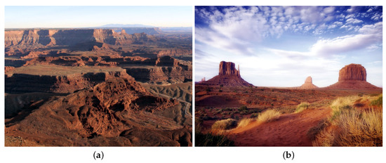
Figure 2. Natural mesa and buttes. Public domain photos found on pxhere.com under the Creative Commons Zero (CC0) license. (a) View of the mesa, Dead Horse Point, Utah, USA. (b) The Mittens (West, East) and Merick Butte, Arizona, USA.

To model such a unique structures, the presented solution uses a terrain constructed from a layered representation (Figure 3). All layers are stored as discrete matrices of numerical values. The first is a geometric layer. It is related to a classic height-field and holds geometric data of the landform and can be defined as a function g: ${\mathbb{R}}^2\to \mathbb{R}$ [18]. The second is a materials layer. It contains information about materials’ distribution, where materials’ classification is related to the elevation records from the geometric layer and can be characterised as a function m: ${\mathbb{R}}^2\to \mathbb{N}$. The last one is a hardness layer. It keeps data about soil resistance to erosion processes and can be described as a function h: ${\mathbb{R}}^2\to \mathbb{R}$.

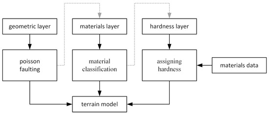
Figure 3. General schema of the proposed terrain model.

2.1. Initial Geometry

The initial geometry of the model can be based on a DEM (Digital Elevation Model) [46] or generated by a procedural method. For the proposed solution, the layer was constructed using a modified Poisson Faulting (or fault formation) algorithm [47]. In a common form, model geometry is divided by random generated lines (fault edges). In the sequential process, one side is raised by a random offset using the step function. In this modification, fault edges are determined by the circular function. The resulting geometry has fBs (fractional Brownian surface) properties [9,20,40]. A rendered comparison of the geometry generated by both variants is presented in Figure 4 and Figure 5.

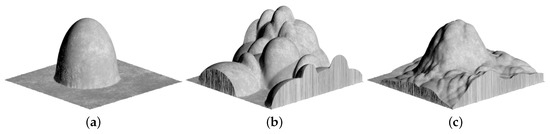
Figure 4. Model generated by circular function of the fault. (Grid resolution: $100\times 100$; fault radius (each): $r=25$; fault height (max in centre): $0\le \Delta h\le 1$). (a) 1 fault. (b) 10 faults. (c) 50 faults.

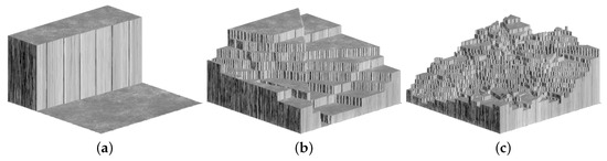
Figure 5. Model generated by linear/step function of the fault. (Grid resolution: $100\times 100$; fault height (each): $\Delta h=1$). (a) 1 fault. (b) 10 faults. (c) 50 faults.

In the article, the linear method is referred to as LFF (Linear Fault Formation) and the circular one as CFF (Circular Fault Formation). The circular fault was selected for three main reasons:

• The LFF combined with a step-based height modifier introduces sharp transitions between points lying on the fault sides, resulting in a rough surface, more adequate in irregular arrangement of rocks and stones than in structured terrain [42];
• The CFF in combination with a new height modifier emulates the distribution of the sediments at the terrain base in the further described erosive procedure;
• The CFF can be limited to a certain area of the height-field, thus the generation of buttes is simplified.

2.1.1. Circular Edge of Fault

The fault divides the geometric layer (G) into two separate subsets of points. Let $p_o=(x_o,y_o)$ be a random point existing in G, so $p_o\in G$. If F is a designated circle with radius r and centre in the point $p_o$, then F determines the edge of the fault that divides G into subsets A and B, where $A\cup B=G$ and $A\cap B=⌀$. The distance (s) of any point $p=(x,y)\in G$ from the fault edge is determined by the circle with centre in the point $p_o$ and radius r:

$$s=r^2-{(x-x_o)}^2-{(y-y_o)}^2$$

(1)

Based on the distance factor, it is possible to evaluate which sides of the fault a point of height-field is located. Let p be any point existing in G, so $p\in G$ and let s be its distance from fault edge (F). Let us assume that $A\subset G$ is a subset of points, where $s>0$ and $B\subset G$ is a subset of points where $s\le 0$. Therefore, we can specify properties of the fault collected in Equation (2) and visualised in Figure 6:

$$p\in \left\{\begin{array}{ccc}A,\hfill & \mathrm{if}\hfill & s>0\hfill \\ B,\hfill & \mathrm{if}\hfill & s\le 0\hfill \end{array}\right.$$

(2)

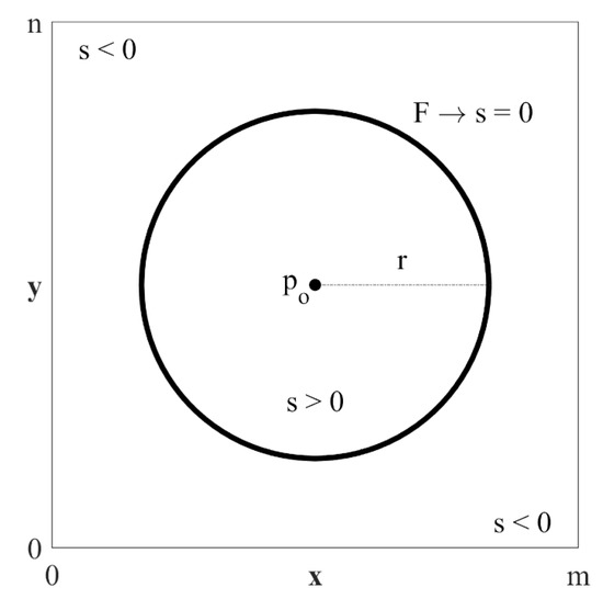
Figure 6. Graphical interpretation of the circular fault properties.

2.1.2. Height Modifier

The modified height position of any point in a geometric layer is related to its distance from the fault edge. The geometry is modified for any point, where $s>0$. To normalise and limit this modification to the interval from $[0,1]\in \mathbb{R}$, the distance is also divided by the fault radius. The height modifier ($\Delta h$) is calculated for each $p\in G$:

$$\Delta h=\left\{\begin{array}{cc}\sqrt{s}/r,\hfill & \mathrm{if}s>0\hfill \\ 0,\hfill & \mathrm{in} \mathrm{other} \mathrm{cases}\hfill \end{array}\right.$$

(3)

The height modifier reaches their maximum limits (value 1.0) for points that positions are identical to $p_o$ and decreases with the increasing distance. Minimum (value 0.0) is reached when the point is on the fault edge or outside it due to the fact that s is not a linear function and $\Delta h$ does not change its value in a linear way. This property was visualised in Figure 7. In the next phase, $\Delta h$ is added to the value in the geometric layer of point $G\left(p\right)$:

$$G^{\prime }\left(p\right)=G\left(p\right)+\Delta h$$

(4)

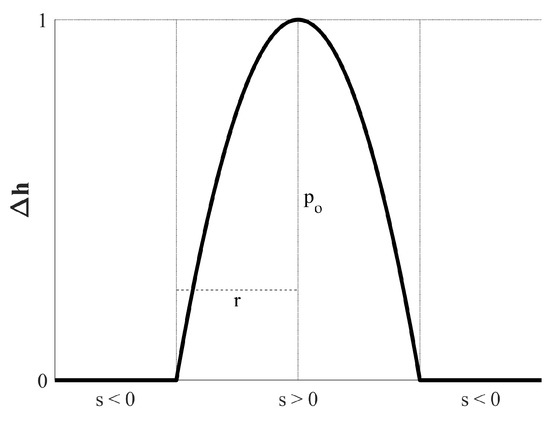
Figure 7. Graph of the height modifier function.

The result of geometry modification by the CFF algorithm is a fBs and for further use it should be normalised to the interval $0\le G\left(p\right)\le 1$, where $G\left(p\right)\in \mathbb{R}$.

2.2. Material Classification

The materials layer (M) stores information about distribution of terrain materials and its basic form is correlated to the model geometry (Figure 3). If $mat$ is a given number of materials assigned to the model, such that $1\le mat\le \infty$, and $mat\in \mathbb{N}$, then each point $p\in M$ can be assigned to a material index where $M\left(p\right)$ means element in the point p:

$$M\left(p\right)=⌊\frac{\lceil 2(mat-1)G\left(p\right)\rceil }{2}⌋$$

(5)

The material layer obtained by the CFF method enables smoother transitions between areas occupied by the individual materials. In contrast, the LFF method is characterised by high irregularity and fraying of the results. The comparison of materials’ distribution for both methods is presented in Figure 8 and Figure 9.

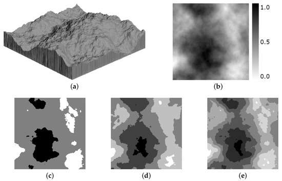
Figure 8. Materials layer generated by the Circular Fault Formation (CFF) method and interpreted as a grey-scale map (grid resolution: $1024\times 1024$; fault radius (each): $r=256$; fault height (max in centre): $0\le \Delta h\le 1$; total faults: 9999). (a) Geometric layer. (b) Initial map. (c) $mat=3$. (d) $mat=5$. (e) $mat=7$.

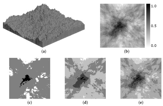
Figure 9. Materials layer generated by the Linear Fault Formation (LFF) method interpreted as a grey-scale map (grid resolution: $1024\times 1024$; fault height (each): $\Delta h=1$; total faults: 9999). (a) Geometric layer. (b) Initial map. (c) $mat=3$. (d) $mat=5$. (e) $mat=7$.

Materials classification is obtained by a quantification of the height values stored in the geometric layer. As an alternative solution, the end-user can choose separately generated fBs as the foundation for the materials classifier. With this approach, materials will not directly correlate with the geometric layer but in relation to the purpose of the article this correlation is preferred.

2.3. Hardness Data

The hardness layer (H) stores information about materials’ hardness (durability) or resistance to the erosion forces and is correlated with the materials’ layers (Figure 3). The binding of materials’ indexes to hardness records can be done by external files or such data can be generated by the normalisation of the materials’ layer. The layer collects data in a range between $0\le H\left(p\right)\le 1$ where $H\left(p\right)$ means the value of the layer in the point p and $H\left(p\right)\in \mathbb{R}$. The value 0.0 means the material is completely vulnerable to erosion and value 1.0 means that it is non-erodible. The numerical value of records can be associated with geological scales of mineral hardness (Table 1) [41]. Entering hardness records completes the initial model preparation (Figure 1).

Table 1. Exemplary comparison of materials’ hardness according to the geological scale of mineral hardness.

Type	Scale of Mineral Hardness
	Absolute	Normalised
none	0	0.0
talc	1	0.001
gypsum	3	0.002
calcite	9	0.006
fluorite	21	0.014
apatite	48	0.032
orthoclase	72	0.048
quartz	100	0.067
topaz	200	0.133
corundum	400	0.267
diamond	1500	1.0

3. Table Mountain Erosion

Long-term landform erosion can be described as the geometrical degradation of a terrain structure that lasted a substantial amount of time. The table mountain structures are forms of thermal, wind, and water erosion where a durable core was exposed by the removal of soft materials. The detached elements are shifted and settled to another location.

The table mountain erosion process, considered in the article, consists of two parts. The first one is general geometry gradation by erosion impact whereas the second one is the levelling of materials. The direct relation of the materials classification and the model geometry ensures the appearance of the stepped sides during the gradation process.

3.1. Geometry Gradation

The proposed method does not simulate dynamic material transportation but is focused on the final results of thermal, rainfall, or hydrological processes, therefore accurate calculations and simulations of sediment dislocation were omitted. This feature was partially included in the CFF algorithm and levelling procedure.

It was assumed that erosion E is a scalar value, such that $0\le E\le 1$, where $E\in \mathbb{R}$ and consists of all erosion phenomena affected on a terrain model over a longer period of time.

The counter-force for erosion is the material’s hardness and reduces its influence. If E is a general erosion force affecting the terrain model, then the gradation factor $\Delta g$ is calculated for each point $p\in G$ in relation to erosion and hardness records $H\left(p\right)$ using Equation (6). Next, $\Delta g$ reduces the value stored in the geometric layer and the gradated value $G^{\prime }\left(p\right)$ is stored in the geometric layer:

$$\Delta g=E\left(1-H\left(p\right)\right)$$

(6)

$$G^{\prime }\left(p\right)=G\left(p\right)-\Delta g$$

(7)

The graphical interpretation of the relation between erosion, hardness, and their impact on the gradation factor is shown in Figure 10. The influence of erosion on the model generated with the CFF method for different numbers of materials is shown in Figure 11.

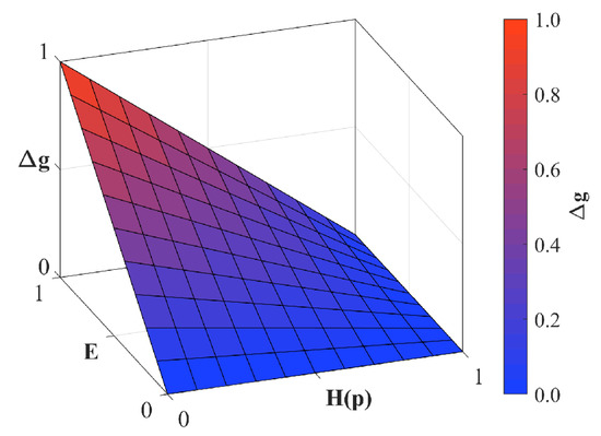
Figure 10. Graphical interpretation of the relation between erosion force, materials’ hardness, and their influence on the results of the gradation factor.

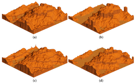
Figure 11. Comparison of the erosion impact on the sample mesa model shown in Figure 8. (a) $E=0.33$, $mat=3$. (b) $E=0.66$, $mat=3$. (c) $E=0.33$, $mat=5$. (d) $E=0.66$, $mat=5$.

Caprock

In addition to the stepped sides, the second significant feature of the table mountains are flat tops. The feature is simulated by setting all points with the highest hardness at the maximum height (in this case the value is 1.0). The impact of this feature for the model is shown in Figure 12.

$$G^{\prime }\left(p\right)=\left\{\begin{array}{cc}1,\hfill & \mathrm{if}H\left(p\right)=1\hfill \\ \mathrm{follow} \mathrm{Equation}\left(7\right),\hfill & \mathrm{in} \mathrm{other} \mathrm{cases}\hfill \end{array}\right.$$

(8)

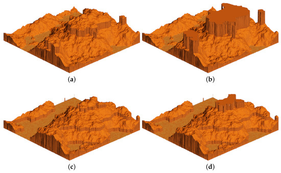
Figure 12. Comparison of the caprock impact on the sample mesa model shown in Figure 8. Erosive model was obtained for $E=0.5$. (a) $mat=3$ without caprock. (b) $mat=3$ with caprock. (c) $mat=5$ without caprock. (d) $mat=5$ with caprock.

3.2. Geometry Levelling

The model obtained by the gradation procedure may have sharp edges between the materials. To reduce this inconvenience, we decided to add a smoothing section, relying on levelling the point geometry to its nearest neighbourhood. The operation can be considered as a variant of Laplacian smoothing based on two-stage average filtering [48]. Firstly, for the selected element of geometric layer $G\left(p\right)$, an average value of its neighbourhood $A_p$ is calculated, but the point itself is not taken into account. Next, an average value is taken from $A_p$ and the point $G\left(p\right)$.

Let $\rho$ be a radius of nearest neighbourhood of $p\in G$, where $0<\rho \le \infty$ and $\rho \in \mathbb{N}$. If $A\subset G$ is a subset of neighbourhood of p, but $p\notin A$ and $A_p$ is a mean height of A, then levelled value $G^{\prime }\left(p\right)$ is an average of $A_p$ and $G\left(p\right)$:

$$G^{\prime }\left(p\right)=\frac{1}{2}(A_p+G\left(p\right))$$

(9)

The transformation of the initial model through gradation and levelling procedures complete the table mountain asset forming (Figure 1). A comparison of the results is shown in Figure 13.

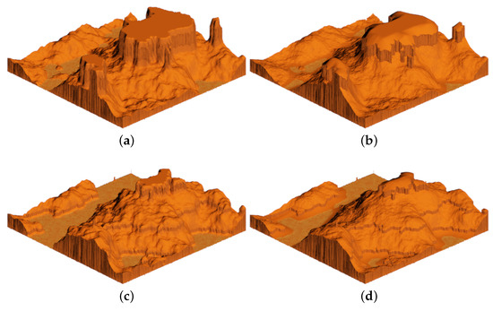
Figure 13. Comparison of the levelling impact on the sample mesa model shown in Figure 12. Erosive model was obtained for $E=0.5$ with caprock. (a) $\rho =10$, $mat=3$. (b) $\rho =50$, $mat=3$. (c) $\rho =10$, $mat=5$. (d) $\rho =50$, $mat=5$.

3.3. Butte Modification

To obtain butte-like structures, it is necessary to modify the way in which the faults are generated. The area available for the next fault is limited to a specified distance around the centre of the geometric layer as shown in Figure 14.

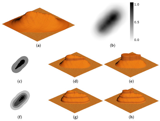
Figure 14. Sample butte generated by circular faults limited along the x-axis (grid resolution: $1024\times 1024$; fault radius: $1\le r\le 350$; total faults: 250). Erosive model was obtained for $E=0.45$ and $\rho =5$. (a) Initial geometry. (b) Initial map. (c) Material layer ($mat=3$) interpreted as a grey-scale map. (d) $mat=3$ without caprock. (e) $mat=3$ with caprock. (f) Material layer ($mat=5$) interpreted as a grey-scale map. (g) $mat=5$ without caprock. (h) $mat=5$ with caprock.

4. Results

The method can be controlled using several attributes, such as the number and radius of the faults, number and hardness of materials, and impact of erosion.

Choosing a too small radius or fault number in relation to the size of the model leads to visually implausible results. In this case, the model has more random peaks or mounds than terrain formation. The experiment shows that a radius greater than $10\%$ of the size of a height-field’s smaller side gives more adequate results then the one out of this range (Figure 15).

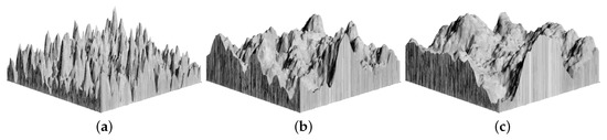
Figure 15. Comparison of the impact of the fault radius on the model geometry (grid resolution: $100\times 100$; fault height (max in centre): $0\le \Delta h\le 1$). (a) $r=3$. (b) $r=10$. (c) $r=25$.

The classification of materials is not limited and theoretically may contain an infinite number, but from a practical side too much value reduces their importance if these are evenly distributed in relation to the model height (Figure 16). However, more materials allow the control of the terrain caprock’s size to a greater extent. By assigning the same hardness to several materials from the top, it is possible to adjust the height of the durable core (Figure 17).

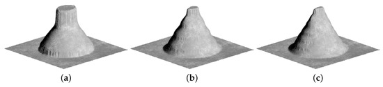
Figure 16. Comparison of the impact of the materials number on the model geometry (grid resolution: $100\times 100$; fault height (max in centre): $0\le \Delta h\le 1$). (a) $mat=3$. (b) $mat=6$. (c) $mat=9$.

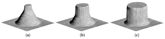
Figure 17. Comparison of the impact of the combination of materials’ hardness on the model geometry shown in Figure 16c. (a) 2 top materials combined. (b) 4 top materials combined. (c) 6 top materials combined.

The experiments show that material hardness selection provides more plausible results if the next one is not less than the previous one, counting from the model base. Omitting this dependence can lead to model calderisation, which is not preferred in table mountains’ modelling (Figure 18).

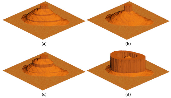
Figure 18. Comparison of the impact of material hardness selection on the model geometry. The model consisted of 5 materials. Hardness values are given in the following order: (a) $0.0;0.25;0.5;0.75;1.0$. (b) $0.0;0.25;0.25;0.25;1.0$. (c) $0.1;0.2;0.3;0.9;1.0$. (d) $0.0;0.25;1.0;0.5;0.9$.

It is worth emphasising that, compared to the LFF, the CFF method is characterised by a plausible reception due to the intended purpose of modelling. The obtained results using the linear version are more adequate for rocky or boulder formations than structured landform. Circular-base results are characterised by less roughness of geometry and better provide the soil sediment arrangement in mesa formations. The main limitation of the method is the problem of an appropriate selection of the radius for the fault circle. It is closely related to the size of the model. A too-small radius leads to unnatural (or rare in nature) results. On a smaller impact, a similar problem also occurs in the case of the wrong selection of the number of faults. Another issue is that the caprock modification provides near-vertical cliffs that can lead to artefacts in the rendering process. Near-vertical structures are generally undesirable in height-field based terrains. This restriction can be removed in volumetric representation.

The example of a textured and rendered butte-like final asset with the application of the proposed approach is presented in Figure 19. Several examples in the orthographic projection of generated mesa-like assets are shown in Figure 20. The butte-like objects are shown in Figure 21.

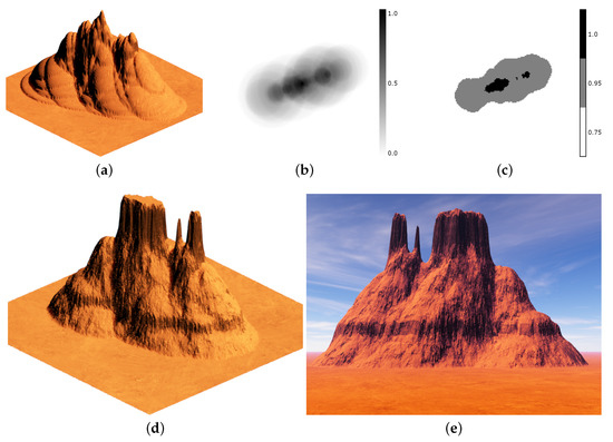
Figure 19. Textured and rendered in a Terragen butte-like asset obtained by the proposed method (grid resolution: $150\times 150$, fault radius: $1\le r\le 35$; total faults: 35 along x-axis). The model consists of 3 materials with following hardness $[0.75;0.95;1.0]$. Erosive model was obtained for $E=0.35$ with caprock and $\varrho =1$. The object feature is similar to the Mittens buttes natural formation in Figure 2b. (a) Plain initial model obtained by the CFF method. (b) Initial map of the model for material classifier. (c) Material layer and hardness records. (d) Orthographic view of the asset. (e) Perspective view of the asset in a virtual environment.

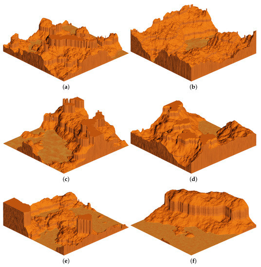
Figure 20. Examples of mesa-like assets obtained by the proposed techniques (grid resolution: $1024\times 1024$). (a) Fault radius: $1\le r\le 350$; total faults: 999; $mat=5$. Erosive model was obtained for $E=0.65$ with caprock and $\varrho =1$. (b) Fault radius: $r=300$ each; total faults: 500; $mat=5$. Erosive model was obtained for $E=0.35$ with caprock and $\varrho =1$. (c) Fault radius: $r=512$ each; total faults: 1500; $mat=5$. Erosive model was obtained for $E=0.75$ with caprock and $\varrho =1$. (d) Fault radius: $r=250$ each; total faults: 2500; $mat=4$. Erosive model was obtained for $E=0.25$ with caprock and $\varrho =10$. (e) Fault radius: $r=250$ each; total faults: 750; $mat=4$. Erosive model was obtained for $E=0.4$ with caprock and $\varrho =2$. (f) fault radius: $r=500$ each; total faults: 3500; $mat=3$. Erosive model was obtained for $E=0.75$ with caprock and $\varrho =5$.

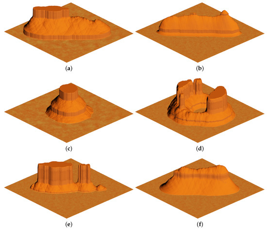
Figure 21. Examples of butte-like assets obtained by the proposed techniques (grid resolution: $1024\times 1024$). (a) Fault radius: $1\le r\le 300$; total faults: 100 along x-axis; $mat=3$. Erosive model was obtained for $E=0.45$ with caprock and $\varrho =1$. (b) Fault radius: $1\le r\le 150$; total faults: 999 along x-axis; $mat=4$. Erosive model was obtained for $E=0.45$ without caprock and $\varrho =25$. (c) Fault radius: $1\le r\le 250$; total faults: 350 around model centre; $mat=4$. Erosive model was obtained for $E=0.30$ with caprock and $\varrho =1$. (d) Fault radius: $1\le r\le 250$; total faults: 150 around model centre; $mat=4$. Erosive model was obtained for $E=0.35$ with caprock and $\varrho =10$. (e) Fault radius: $1\le r\le 250$; total faults: 75 along x-axis; $mat=4$. Erosive model was obtained for $E=0.65$ with caprock and $\varrho =5$. (f) Fault radius: $1\le r\le 250$; total faults: 250 along x-axis; $mat=3$. Erosive model was obtained for $E=0.35$ without caprock and $\varrho =5$.

4.1. Testing Workstation and Applications

All results were received using prototype application Terax 2.0 compiled in Microsoft Visual Studio 2013. The software was partly written in C# 5.0, C++11, and CUDA 3.5 for Microsoft Windows x64 platform. However, all algorithms were tested on the GPU implementation. For random sequences, the Mersenne Twister algorithm in 64-bit variant was used. The testing workstation was based on the Asus Maximus VI Formula motherboard equipped with Intel Core i7-4771 CPU, 32 GB Kingston Hyper-X DDR3 RAM, and Asus GTX780-DC2OC-3GD5 Graphics Card with nVidia GeForce GTX 780 GPU. The visualisation was performed in Terragen 3.4 Professional Edition with Animation (Planetside Software LLC) without any of the application-specific modifiers except colour shaders.

4.2. Computational Efficiency

The estimation of the computational efficiency of the proposed technique was considered separately for geometric and materials layers.

In theory, the faulting algorithm complexity should be interpreted as $O(m\times n^2)$ for square height-fields defined as two-dimensional matrices (side n). It depends on the model size ($n\times n$) and m as the number of faults (data processing needs two nested loops for introducing each fault). Our experiments, with the practical implementation for large models, showed that the faults number has much less influence on computation time in comparison to model size. This lead us to further examinations and the introduction of the concept of height-field as a one-dimensional vector (only one loop is required then to process data for each fault). With a limited constant value of m, it may be assumed that the overall cost of the (practical) method can be considered as linear dependency.

The CFF geometry modelling performance was tested in comparison to the LFF and the impact of the model size. For both methods, the test sample consisted of 100 models per n-size, where $n=(1,\dots ,9)\times {10}^6$ and $n\in \mathbb{N}$. All models were seeded by randomised value with a uniform distribution and generated by 1000 faults with a constant height ($1.0$). The radius for circular fault was also constant and set to $r=250$. The results indicate the linear character of the method in terms of the size of the model. The results presented in Table 2 and in Figure 22 show that for the largest models tested, the working time did not exceed $0.3$ s. In general, the CFF method is faster than the LFF technique due to the fact that the fault area is definitely smaller. Only in the worst case scenario, the efficiency of the proposed method will be equal to the linear one. However, the choice of the radius for which the faults would cover an area comparable to the LFF method is not the purpose of the publication.

Table 2. Computational efficiency of the CFF method depending on the model size compared to the LFF variant.

Model Size		Geometry
Elements	Resolution	LFF	CFF
$\mathbf{\times }{\mathbf{10}}^{\mathbf{6}}$	$\mathbf{\times }{\mathbf{10}}^{\mathbf{3}}$	t [ms]	t [ms]
1	$1\times 1$	53	38
2	$2\times 1$	99	69
3	$2\times 1.5$	145	100
4	$2\times 2$	191	132
5	$2.5\times 2$	236	163
6	$3\times 2$	281	195
7	$7\times 1$	327	227
8	$4\times 2$	372	258
9	$3\times 3$	416	290

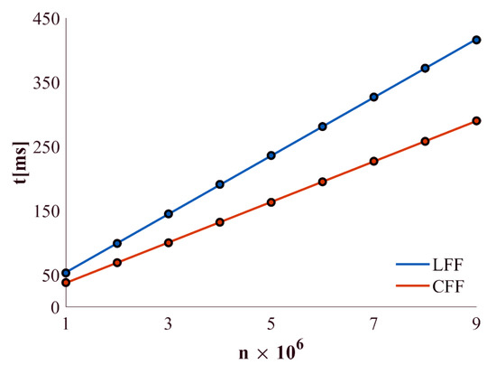
Figure 22. Computational efficiency of the CFF method depending on the model size compared to the LFF variant.

The experiments also include the influence of the model size on the materials’ classification. Within it, 100 models were examined per n-size, where $n=(1,\dots ,9)\times {10}^6$ and $n\in \mathbb{N}$. All models were generated for 1000 faults with a constant radius $r=250$ and seeded by randomised value with a uniform distribution. The initial models consist of materials for $mat=(2,\dots ,255)$, where $mat\in \mathbb{N}$. In total, $2277\times {10}^4$ models were tested. The results show the linear nature of the classification method in terms of the model size and for the largest models tested, the working time did not exceed 0.02 s. The results are summarised in Table 3 and shown in Figure 23a.

Table 3. Computational efficiency of the proposed techniques depending on the model size.

Model Size
Elements	Resolution	Materials	Erosion
$\mathbf{\times }{\mathbf{10}}^{\mathbf{6}}$	$\mathbf{\times }{\mathbf{10}}^{\mathbf{3}}$	t [ms]	t [ms]
1	$1\times 1$	2	7
2	$2\times 1$	4	13
3	$2\times 1.5$	6	18
4	$2\times 2$	8	24
5	$2.5\times 2$	9	30
6	$3\times 2$	11	36
7	$7\times 1$	13	42
8	$4\times 2$	14	47
9	$3\times 3$	16	53

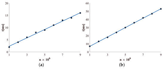
Figure 23. Computational efficiency of the proposed techniques. (a) Material classification. (b) Model gradation.

The influence of the model size on the erosion modifier was also examined. Within it, 100 models were tested per n-size, where $n=(1,\dots ,9)\times {10}^6$ and $n\in \mathbb{N}$. All models were generated by 1000 faults with constant radius $r=250$ and seeded by randomised value with a uniform distribution. For the procedure, $mat=9$ as the materials number was selected. The initial models were eroded for $E=(0.1,0.2,\dots ,0.9)$, where $E\in \mathbb{R}$. In total, 8100 models were tested. The results show the linear nature of the erosion process in terms of the model size and for the largest models tested, the working time did not exceed 0.06 s. The results were collected in Table 3 and shown in Figure 23b.

5. Conclusions

This article introduced a new technique for the modelling of table mountains based on the internal structure of the terrain and circular fault formation algorithm. The presented model contained classic height-field extended by information about the distribution, placement, and hardness of materials that the landscape consists of. The main contribution of the proposed technique is a fast, not simulation-oriented method (Figure 1) that enables one to obtain height-field based, stepped sides terrain assets that can be imported into any virtual environment to be used by artist or level designers. The proposed algorithms are easy to implement in both CPU and GPU oriented programming and lead to expected results controllable by several parameters. The end user can freely choose the number of materials and their hardness and observe changes in the geometry of the model in real-time. The algorithm could be a part of an interactive tool for creating mesa and butte objects in modelling applications or game engines.

Future work will focus on volumetric models and the ability to generate more complex forms of terrain including arches or rock shelves [8,17]. A terrain model with materials’ deposition and hardness data in simulation of fast progressing erosive phenomena like mud- or landslides should also be analysed [49].

References

- Frade, M.; de Vega, F.; Cotta, C. Modelling Video Games’ Landscapes by Means of Genetic Terrain Programming: A New Approach for Improving Users’ Experience. In Applications of Evolutionary Computing; Giacobini, M., Brabazon, A., Cagnoni, S., Di Caro, G.A., Drechsler, R., Ekárt, A., Esparcia-Alcázar, A.I., Farooq, M., Fink, A., McCormack, J., et al., Eds.; Lecture Notes in Computer Science; Springer: Berlin/Heidelberg, Germany, 2008; Volume 4974, pp. 485–490. [Google Scholar]
- Roman, P.A.; Brown, D. Games—Just how serious are they? In Proceedings of the Interservice/Industry Training, Simulation, and Education Conference (I/ITSEC ’08), Orlando, FL, USA, 1–5 December 2008; pp. 1–11. [Google Scholar]
- Wells, W.D.; Darken, C.J. Generating enhanced natural environments and terrain for interactive combat simulations (GENETICS). In Proceedings of the ACM Symposium on Virtual Reality Software and Technology (VRST ’05), Monterey, CA, USA, 7–9 November 2005; pp. 184–191. [Google Scholar]
- Wilkowski, A.; Kornuta, T.; Stefańczyk, M.; Kasprzak, W. Efficient generation of 3D surfel maps using RGB–D sensors. Int. J. Appl. Math. Comput. Sci. 2016, 26, 99–122. [Google Scholar] [CrossRef]
- Guérin, E.; Digne, J.; Galin, E.; Peytavie, A.; Wolf, C.; Beneš, B.; Martinez, B. Interactive Example-based Terrain Authoring with Conditional Generative Adversarial Networks. ACM Trans. Graph. 2017, 36, 228. [Google Scholar] [CrossRef]
- Bézin, R.; Crespin, B.; Skapin, X.; Terraz, O.; Meseure, P. Generalized Maps for Erosion and Sedimentation Simulation. Comput. Graph. 2014, 45, 1–16. [Google Scholar] [CrossRef]
- Génevaux, J.D.; Galin, E.; Guérin, E.; Peytavie, A.; Beneš, B. Terrain Generation Using Procedural Models Based on Hydrology. In Proceedings of the Annual Conference on Computer Graphics and Interactive Techniques (SIGGRAPH ’13), Anaheim, CA, USA, 21–25 July 2013; pp. 1–13. [Google Scholar]
- Beneš, B.; Forsbach, R. Layered data representation for visual simulation of terrain erosion. In Proceedings of the Spring Conference on Computer Graphics (SCCG ’01), Budmerice, Slovakia, 25–28 April 2001; pp. 80–85. [Google Scholar]
- Musgrave, F.K. Methods for Realistic Landscape Imaging. Ph.D. Thesis, Yale University, New Haven, CT, USA, 1993. [Google Scholar]
- Musgrave, F.K.; Kolb, C.E.; Mace, R.S. The synthesis and rendering of eroded fractal terrains. In Proceedings of the Annual Conference on Computer Graphics and Interactive Techniques (SIGGRAPH ’89), Boston, MA, USA, 31 July– 4 August 1989; pp. 41–50. [Google Scholar]
- Št’ava, O.; Beneš, B.; Brisbin, M.; Křivánek, J. Interactive Terrain Modeling Using Hydraulic Erosion. In Proceedings of the ACM SIGGRAPH/Eurographics Symposium on Computer Animation (SCA ’08), Dublin, Ireland, 7–9 June 2008; pp. 201–210. [Google Scholar]
- Cordonnier, G.; Braun, J.; Cani, M.P.; Beneš, B.; Galin, E.; Peytavie, A.; Guérin, E. Large Scale Terrain Generation from Tectonic Uplift and Fluvial Erosion. Comput. Graph. Forum 2016, 35, 165–175. [Google Scholar] [CrossRef]
- Cordonnier, G.; Cani, M.P.; Beneš, B.; Braun, J.; Galin, E. Sculpting Mountains: Interactive Terrain Modeling Based on Subsurface Geology. IEEE Trans. Vis. Comput. Graph. 2018, 24, 1756–1769. [Google Scholar] [CrossRef] [PubMed]
- Beneš, B.; Arriaga, X. Table Mountains by Virtual Erosion. In Proceedings of the Eurographics Workshop on Natural Phenomena (NPH ’05), Dublin, Ireland, 30 August 2005; pp. 33–39. [Google Scholar]
- Smelik, R.M.; de Kraker, K.J.; Tutenel, T.; Bidarra, R.; Groenewegen, S.A. A survey of procedural methods for terrain modelling. In Proceedings of the CASA Workshop on 3D Advanced Media in Gaming and Simulation (3AMIGAS ’09), Amsterdam, The Netherlands, 16 June 2009; pp. 25–34. [Google Scholar]
- Smelik, R.M.; Tutenel, T.; Bidarra, R.; Beneš, B. A Survey on Procedural Modelling for Virtual Worlds. Comput. Graph. Forum 2014, 33, 31–50. [Google Scholar] [CrossRef]
- Lengyel, E.S. Voxel-Based Terrain for Real-Time Virtual Simulations. Ph.D. Thesis, University of California, Davis, CA, USA, 2010. [Google Scholar]
- Galin, E.; Guérin, E.; Peytavie, A.; Cordonnier, G.; Cani, M.P.; Beneš, B.; James, G. A Review of Digital Terrain Modeling. Comput. Graph. Forum 2019, 38, 553–577. [Google Scholar] [CrossRef]
- Schmitter, D.; García-Amorena, P.; Unser, M. Smooth Shapes with Spherical Topology: Beyond Traditional Modeling, Efficient Deformation, and Interaction. Comput. Vis. Media 2017, 3, 199–215. [Google Scholar] [CrossRef]
- Mandelbrot, B.B.; Van Ness, J.W. Fractional Brownian motions, fractional noises and applications. SIAM Rev. 1968, 10, 422–437. [Google Scholar] [CrossRef]
- Mandelbrot, B.B. Stochastic models for the earth’s relief, the shape and fractal dimension of coastlines, and the number area rule for islands. Proc. Natl. Acad. Sci. USA 1975, 72, 2825–2828. [Google Scholar] [CrossRef]
- Mandelbrot, B.B. The Fractal Geometry of Nature, 2nd ed.; H.W. Freeman and Co.: San Francisco, CA, USA, 1982. [Google Scholar]
- Voss, R.F. Random Fractal Forgeries. In Fundamental Algorithms for Computer Graphics; Earnshaw, R.A., Ed.; NATO ASI Series; Springer: Berlin, Germany, 1991; Volume 17, pp. 805–835. [Google Scholar]
- Ebert, D.S.; Musgrave, F.K.; Peachery, D.; Perlin, K.; Worley, S. Texture & Modeling: A Procedural Approach, 3rd ed.; The Morgan Kaufmann Series in Computer Graphics and Geometric Modeling; Morgan Kaufmann Publishers: San Francisco, CA, USA, 2003. [Google Scholar]
- Prusinkiewicz, P.; Hammel, M. A Fractal Model of Mountains with River. In Proceedings of the Graphics Interface (GI ’93), Toronto, ON, Canada, 19–21 May 1993; pp. 174–180. [Google Scholar]
- Nagashima, K. Computer generation of eroded valley and mountain terrains. Vis. Comput. 1997, 13, 456–464. [Google Scholar] [CrossRef]
- Van Lawick van Pabst, J.; Jense, H. Dynamic Terrain Generation Based on Multifractal Techniques. In Proceedings of the International Workshop on High Performance Computing for Computer Graphics and Visualisation, Swansea, UK, 3–4 June 1995; pp. 186–203. [Google Scholar] [CrossRef]
- Zuo, C.; Wu, L.; Zeng, Z.F.; Wei, H.L. Stochastic fractal based multiobjective fruit fly optimization. Int. J. Appl. Math. Comput. Sci. 2017, 27, 417–433. [Google Scholar] [CrossRef]
- Kristof, P.; Beneš, B.; Krivanek, J.; Stava, O. Hydraulic Erosion Using Smoothed Particle Hydrodynamics. Comput. Graph. Forum 2009, 28, 219–228. [Google Scholar] [CrossRef]
- Beneš, B.; Těšínský, V.; Hornyš, J.; Bhatia, S.K. Hydraulic erosion. Comput. Animat. Virtual Worlds 2006, 17, 99–108. [Google Scholar] [CrossRef]
- Beneš, B. Real-Time Erosion Using Shallow Water Simulation. In Proceedings of the Workshop in Virtual Reality Interactions and Physical Simulation (VRIPHYS ’07), Dublin, Ireland, 9–10 November 2007; pp. 43–50. [Google Scholar]
- Beneš, B.; Forsbach, R. Visual Simulation of Hydraulic Erosion. In Proceedings of the International Conferences in Central Europe on Computer Graphics, Visualization and Computer Vision (WSCG ’02), Plzen-Bory, Czech Republic, 4–8 February 2002; pp. 79–86. [Google Scholar]
- Natali, M.; Lidal, E.M.; Parulek, J.; Viola, I.; Patel, D. Modeling Terrains and Subsurface Geology. In Proceedings of the EUROGRAPHICS State of the Art Reports (STAR ’12), Cagliary, Italy, 13–18 May 2012; pp. 155–173. [Google Scholar] [CrossRef]
- Frade, M.; de Vega, F.F.; Cotta, C. Breeding terrains with genetic terrain programming: The evolution of terrain generators. Int. J. Comput. Games Technol. 2009, 83–96. [Google Scholar] [CrossRef]
- Golubev, K.; Zagarskikh, A.; Karsakov, A. Dijkstra-based Terrain Generation Using Advanced Weight Functions. In Proceedings of the 5th International Young Scientist Conference on Computational Science (YSC ’16), Kraków, Poland, 26–28 October 2016; pp. 152–160. [Google Scholar]
- Génevaux, J.D.; Galin, E.; Peytavie, A.; Guérin, E.; Briquet, C.; Grosbellet, F.; Beneš, B. Terrain Modelling from Feature Primitives. Comput. Graphics Forum 2015, 34, 198–210. [Google Scholar] [CrossRef]
- Zawadzki, T.; Nikiel, S.; Warszawski, K. Hybrid of shape grammar and morphing for procedural modeling of 3D caves. Trans. GIS 2012, 16, 619–633. [Google Scholar] [CrossRef]
- Shankel, J. Fractal terrain generation—Particle deposition. In Game Programming Gems; DeLoura, M.A., Ed.; Charles River Media: Rockland, MA, USA, 2000; Volume 1, pp. 508–511. [Google Scholar]
- Warszawski, K.; Nikiel, S. A proposition of particle system-based technique for automated terrain surface modeling. In Proceedings of the 5th International North American Conference on Intelligent Games and Simulation (Game-On-NA ’09), Atlanta, GA, USA, 26–28 August 2009; pp. 17–19. [Google Scholar]
- Fournier, A.; Fussell, D.; Carpenter, L. Computer rendering of stochastic models. Commun. ACM 1982, 25, 371–384. [Google Scholar] [CrossRef]
- Mukherjee, S. Applied Mineralogy: Applications in Industry and Environment; Springer: Dordrecht, The Netherlands, 2011. [Google Scholar]
- Migoń, P.; Różycka, M.; Jancewicz, K.; Duszyński, F. Evolution of sandstone mesas—Following landform decay until death. Prog. Phys. Geogr. 2018, 42, 588–606. [Google Scholar] [CrossRef]
- Waters, R. Differential Weathering and Erosion on Oldlands. R. Geogr. Soc. 1957, 123, 503–509. [Google Scholar] [CrossRef]
- Lewis, R.Q.; Trimble, D.E. Geology and and Uranium Deposits of Monument Valley, San Juan County, Utah; Technical Report 1087, Geological Survey Bulletin; United States Department of the Interior: Washington, DC, USA, 1959.
- Baker, A.A. Geology of the Monument Valley–Navajo Mountain Region, San Juan County, Utah; Technical Report 865, Geological Survey Bulletin; United States Department of the Interior: Washington, DC, USA, 1936.
- Chen, X.; Sun, Q.; Hu, J. Generation of Complete SAR Geometric Distortion Maps Based on DEM and Neighbor Gradient Algorithm. Appl. Sci. 2018, 8, 2206. [Google Scholar] [CrossRef]
- Shankel, J. Fractal terrain generation—Fault formation. In Game Programming Gems; DeLoura, M.A., Ed.; Charles River Media: Rockland, MA, USA, 2000; Volume 1, pp. 499–502. [Google Scholar]
- Vollmer, J.; Mencl, R.; Müller, H. Improved Laplacian Smoothing of Noisy Surface Meshes. Comput. Graph. Forum 1999, 18, 131–138. [Google Scholar] [CrossRef]
- Park, S.; Kim, J. Landslide Susceptibility Mapping Based on Random Forest and Boosted Regression Tree Models, and a Comparison of Their Performance. Appl. Sci. 2019, 9, 942. [Google Scholar] [CrossRef]
© 2019 by the authors. Licensee MDPI, Basel, Switzerland. This article is an open access article distributed under the terms and conditions of the Creative Commons Attribution (CC BY) license (http://creativecommons.org/licenses/by/4.0/).