Abstract
In the uncooled infrared imaging systems, owing to the non-uniformity of the amplifier in the readout circuit, the infrared image has obvious stripe noise, which greatly affects its quality. In this study, the generation mechanism of stripe noise is analyzed, and a new stripe correction algorithm based on wavelet analysis and gradient equalization is proposed, according to the single-direction distribution of the fixed image noise of infrared focal plane array. The raw infrared image is transformed by a wavelet transform, and the cumulative histogram of the vertical component is convolved by a Gaussian operator with a one-dimensional matrix, in order to achieve gradient equalization in the horizontal direction. In addition, the stripe noise is further separated from the edge texture by a guided filter. The algorithm is verified by simulating noised image and real infrared image, and the comparison experiment and qualitative and quantitative analysis with the current advanced algorithm show that the correction result of the algorithm in this paper is not only mild in visual effect, but also that the structural similarity (SSIM) and peak signal-to-noise ratio (PSNR) indexes can get the best result. It is shown that this algorithm can effectively remove stripe noise without losing details, and the correction performance of this method is better than the most advanced method.
1. Introduction
Infrared imaging has been widely used in military, agricultural, and medical applications. However, owing to the defects of focal plane array materials and manufacturing limitations [1], the response of the infrared focal plane array unit is inconsistent, and serious spatial fixed pattern noise (FPN) is generated in the infrared image [2]. In engineering applications, people usually use traditional methods to correct FPN noise, in addition to FPN, random noise is also a part of the noise of the infrared image, and its energy is usually smaller than FPN. Random noise is composed of 1/f noise, thermal noise, bias voltage noise and so on. After the system is subjected to traditional non-uniformity correction, the FPN will be reduced, and random noise will become the main noise [3]. For uncooled infrared focal plane array (FPA), the FPA usually consists of a detector array, readout circuit and an analog-to-digital converter as shown in Figure 1a, where the non-uniformity of the readout circuit will also generate column FPN. Without certain noise compensation, the column FPN will appear as obvious vertical strips in a raw infrared image, as shown in Figure 1b [4]. To improve the quality of infrared images, stripe non-uniformity correction is required.
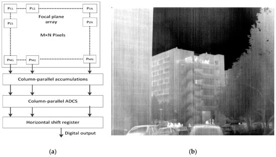
Figure 1.
Readout circuits in infrared focal plane array (FPA) have different characteristics and such non-uniformity will generate column fixed pattern noise (FPN). (a) Block diagram of Uncooled Long-Wave infrared. (b) A raw infrared image which contains obvious stripe noise (The image is available under the Creative Commons Attribution (CC-BY) license [9]).
Currently, the mainstream non-uniform correction (NUC) methods are calibration correction [5,6] and scene-based correction [7,8]. The calibration correction requires periodic interruption of the system’s operation to eliminate the effects of temperature drift and then the calibration parameters cannot be updated in real time. The calibration correction generally handles non-uniformities caused by differences in response units and is not suitable for correcting stripe noise. By contrast, the scene-based correction does not require black body calibration, and extracts parameters based on scene information. As a result, it has attracted considerable attention.
Scene-based correction may be either multi-frame or single-frame. The single frame method has a high convergence rate and can correct the stripe non-uniformity from the first frame. Currently, a single frame algorithm with better effect of removing stripe noise has been proposed by Sui et al. namely an NUC algorithm based on grayscale inheritance [3]. However, it is difficult to determine an appropriate threshold; moreover, the algorithm is complex, which limits its applicability. Tendero et al. proposed a midway histogram equalization [9]. However, this method does not consider stripe noise characteristics, and thus the details and edge information of the image are blurred to some extent when the stripes are removed. Therefore, if the raw infrared image has low contrast, fuzzy results are obtained. Cao et al. proposed a wavelet stripe correction algorithm [1], which performs a three-level size decomposition on the image and filters on each level. The algorithm is complex and the denoising effect is not ideal. Qian put forward a method that minimizes the mean square error [10]. Although stripe noise is removed well, loss of image details often occurs.
To resolve these issues, a new destriping algorithm that minimizes the horizontal gradient of the image is proposed in the present study. First, a wavelet transform is applied to the raw infrared image, and a Gaussian operator is used to convolve the cumulative histogram of the vertical component with a one-dimensional matrix to achieve gradient equalization in the horizontal direction. In addition, the vertical component is used as an input and a guided filter is used for double filtering, thus removing noise and simultaneously retaining image details.
The main contribution of this research is to propose a multi-scale correction method. Firstly, the algorithm is based on the single frame image NUC algorithm, and thus does not need to process multiple frames of images and cause unnecessary “ghosting” problems. Secondly, the algorithm directly denoises the vertical component, which can accurately remove the stripe noise and preserve the details of the image. Experiments show that our algorithm is superior to the current advanced stripe correction algorithm on both simulated images and raw infrared images.
This paper is organized as follows: in the Section 2, the related work of non-uniform correction algorithm is introduced. In the Section 3, a new infrared image non-uniform stripe correction algorithm is proposed and the implementation details of the algorithm are given in the Section 4. The experimental results of the correction algorithm are given in the Section 5. Finally, the conclusion is drawn in the Section 6.
2. Related Work
The spatial non-uniformity of infrared FPA detector arises from the defects of the focal plane array material and manufacturing process, which leads to the inconsistent response of the infrared focal plane array unit. Generally, this can be corrected by calibration method, but the calibration method is not applicable to stripe noise. The most fundamental NUC technology is based on radiation calibration. For instance, the two-point correction method enables the detector to calculate a set of independent correction factors (gain and offset) through radiation correction at the same temperature. The model is simple and the calculation is convenient. However, this method requires periodic interruption of the system’s operation and real-time correction of the system cannot be achieved. In order to overcome this shortcoming, a large number of NUC algorithms based on time–domain filtering and scene information are proposed [7,11,12,13]. However, the limitation of this type of scene algorithm is that it requires stable correction factors for multi-frame images, so it is difficult to implement the algorithm in hardware. Moreover, the scene-based NUC algorithm requires the image to have sufficient scene motion; otherwise the image will be rendered with “ghosting” problems.
Recently, a large number of single-frame NUC algorithms have been proposed [14,15]. These algorithms usually divide the image into high-frequency parts and smooth parts, and denoise the high-frequency parts. However, in reality, if the texture information of the image is insufficient, it is very difficult to separate the noise and the texture of the image. In general, in the denoising method of filtering (bilateral filtering and guided filtering) [16,17,18], a threshold value should be set to distinguish the edge and noise, to achieve the effect of edge preservation. However, when the image texture information is weak, the algorithm may erroneously remove the texture information as noise or save the stripe noise with large amplitude as texture information. In the statistical gray correction algorithm [9,19,20], it assumes that the histograms of adjacent columns are the same, and the histogram information of the columns is modified by the adjacent histogram relationship. Conversely, in the constrained optimization method [21,22], it is assumed that the stripe noise affects the horizontal direction gradient and has little effect on the vertical direction gradient, so, the problem is converted to minimizing the energy function. With the application of convolutional neural networks in image processing in recent years, Kuang et al. [23] proposed a deep convolutional neural network (CNN) model to correct the non-uniformity of infrared images, which can accurately remove stripe noise.
3. Stripe Correction New Algorithm Based on Wavelet Analysis and Gradient Equalization
The proposed algorithm includes the following three steps: (1) Wavelet decomposition of the original image to extract high-frequency components, and then the stripe noise is concentrated in the vertical component of the high-frequency component. (2) Small-window column equalization of vertical components. (3) Taking the approximate component as the guidance image, and the equalization vertical component as the input image, then using the guided filter for the second filtering, and finally carrying out the wavelet reconstruction. The complete flow chart of the algorithm is shown in Figure 2. The details of the proposed method are presented in the following subsections.
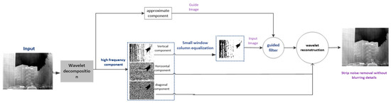
Figure 2.
Workflow of our proposed algorithm. Please zoom in to check details.
3.1. Wavelet-Based Image Decomposition
Wavelet analysis is a rapidly developing area in mathematics and engineering. It has been successfully applied in several fields. Originating in Fourier analysis, the wavelet transform has the characteristics of multi-scale analysis and the ability to represent the local characteristics of signals in both time and frequency domains. Thus, it can effectively extract information from signals [1,24]. In image denoising algorithms, the wavelet transform can generate multi-scale representation of the input image. One of the most important properties of the wavelet transform is that the information in different directions of the image can be decomposed into corresponding components. Zhe et al. [25,26] proposed an image cartoon-texture decomposition and sparse representation algorithm, which decomposes the image into cartoon parts and texture parts, and uses sparse representation in the texture part of the image, which can preserve the texture information of the image well. But the noise of the infrared stripes mainly exists in the vertical direction, and so therefore, we choose wavelet decomposition to represent the information of different directions of the image.
In image denoising, continuous small waves and their wavelet transform should be discretized [8,24]. Mathematically, this is defined as:
where represents the sampling interval, m represents the sampling scale. m and n take integers. Formula (1) is the discrete wavelet function. Then the discrete wavelet transform [1,8] of g(t) is:
In order for the wavelet transform to capture the variability of spatial and frequency resolution, a dynamic sampling grid is adopted, and a binary wavelet is commonly used to realize the function of signal zoom analysis. In Formula (3), n corresponds to in Formula (1):
The wavelet transform extracts high frequency components from the original image , and the formula is:
According to Formula (4), the high-frequency components not only contain stripe noise , but also vertical texture information . After wavelet decomposition, the signal is expressed as:
where represents the approximate component, the horizontal component, the vertical component, and the diagonal component. It can be clearly observed from Figure 3 that stripe noise is concentrated in the vertical component. According to this experimental conclusion, stripe noise can be eliminated directly in the vertical component. We tested three different wavelet bases: db1 wavelet, haar wavelet, and sym8 wavelet. Our proposed method chooses three wavelet basis functions for experiments, and the results are shown in Figure 4. It can be seen from the highlighting in the figure that the haar wavelet and the sym8 wavelet cause “ghosting” problems. The db1 wavelet preserves the vertical texture information of the image well.
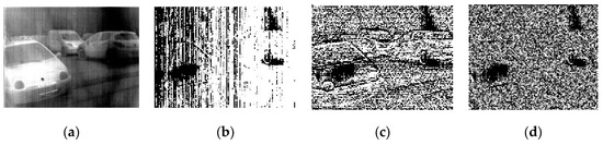
Figure 3.
Wavelet decomposition: (a) original image, (b) vertical component, (c) horizontal component, and (d) diagonal component. Please zoom in to check details.
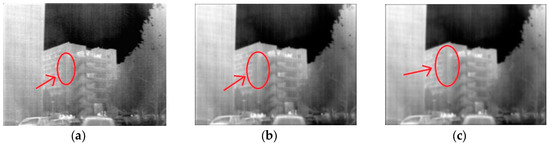
Figure 4.
From left to right (a) using db1 wavelet, (b) using haar wavelet, (c) using sym8 wavelet. Please zoom in to check details.
3.2. Small Window Column Equalization
Currently, the readout circuit of an uncooled infrared imaging system mostly adopts the CMOS architecture. Different from the CCD structure in which all pixels share a common amplifier, the pixels in each column of the CMOS readout circuit share an amplifier [27]. As amplifiers have different electronic properties, the columns of the CMOS readout circuit are non-uniform and thus appear as stripes in the image. In infrared image non-uniformity correction algorithms, the response of infrared focal plane pixels is generally approximated by a linear model, as follows:
where Yn(i,j) is the output of the detector, Xn(i,j) is the true response value of the detector, an(i,j) and bn(i,j) are the gain and bias coefficients, and n is the number of frames in the image sequence.
Considering that the stripe noise in the image is a fixed additive noise, the infrared image model can be simplified as follows:
where (i,j) are pixel coordinates, and Yn(i,j) represents infrared images containing vertical stripes noise. E(j) is a one-dimensional vector whose elements correspond to the vertical stripe noise of each column of the image. The effect of stripe noise on the image gradient is mainly concentrated in the horizontal direction, whereas the gradient in the vertical direction is hardly affected. Based on the above theoretical basis, infrared noise can be removed by reducing the horizontal gradient.
Assuming that each column of a single infrared image contains sufficient information, and that the image is continuous, the gray value between two adjacent columns does not change significantly, and denoising can be achieved by equalizing the column histogram. Calculate the cumulative histogram Hj of each column pixel Uj of the vertical component, and for the cumulative histogram data H(i,j) of the entire image U, Formula (8) is used to perform horizontal convolution on the cumulative histogram of the vertical component to achieve column equalization:
where denotes convolution, and N is the operation range. A Gaussian kernel function is used to generate the one-dimensional matrix W(i,j) with size 1 × (2N + 1), as follows:
The value N for the window is selected as 1. The value of φ is only related to inherent detector characteristics, and it can be obtained through pre-calibration. In this study, an optimized structure is introduced to add a total variational regular term and adaptively determine the value of . The formula is as follows:
where is the image after correction for a specific value of variance. The total variation of is defined as follows [22]:
The value of can be obtained as follows: First, the chooses a smaller value, and then increase the value of , and constantly observes the quality of the image, when the image quality is the highest, then the value of is the detector’s variance. When the value of window N is fixed at 1, as shown in Figure 5, if is taken as a small value, there will be a large quantity of stripe noise residuals. When is increased to a certain value, the image will appear blurred, and the experimental results show that we choose the parameter = 5.
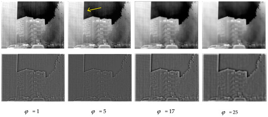
Figure 5.
Top: The vertical component using different values for column gradient equalization. Bottom: the recovered image high frequency. If we set to a small value ( = 1), strip noise cannot be well separated from image texture. If we set to a large value ( = 17 or 25), the output image is blurred. In our implementation we set = 5. Please zoom in to check details.
3.3. Guide Filtering Removes Vertical Component Noise
Guided filter uses guidance image to destriping the input image . Local linear model of guided filter assumes that filtered output q is a linear transform of the guidance I. Therefore, guidance image directly affects the output [18,28]. The formula defined between the two is as follows:
where and are continuous linear constant coefficients in window . is the guidance image, is a window centered at pixel k, The constraint equations for and in window are:
where is a regularization parameter, the purpose is to make converge.
By minimizing the constraint equation to minimize the deviation between the input image and the output image, the coefficients and are:
where and are the mean and variance of the guidance image in the window , is the mean of the input image in window . is the number of pixels in window .
According to the formula, if the regularization parameter is given, the size of filtering window h will affect the output of guided filtering. In this paper, H represents the height of the image. Figure 6 shows the results of using different window sizes. If we set the window sizes h to a low value, many obvious stripes noise still remain visible in the smoothed output, as shown in Figure 6b. Conversely, setting the value of h to a large value, there will be obvious fuzzy phenomenon in Figure 6d,e, as highlighted in yellow. In our experiment, h = 0.3H was used, and the regularization parameter was 0.22.
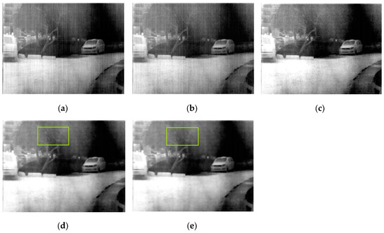
Figure 6.
Stripe removal results with different window heights. From left to right (a) Raw infrared image (b) h = 0.1H, (c) h = 0.3H, (d) h = 0.5H, (e) h = 0.7H. H denotes the height of the image. Regularization parameter is set to 0.22. Please zoom in to see details in the pictures.
4. Implementation Details
In this section, we provide the implementation details of the algorithm. First, the considerations of wavelet decomposition, column gradient equalization, and guided filter are elaborated. Then the entire procedure is used as a quick reference.
4.1. Detail Description
For the M × N size image (M and N default to an even number), after db1 wavelet base decomposition, the image becomes half of the original image size (M/2 × N/2). In the process of column gradient equalization, to avoid losing image details, the window value is 1 and the one-dimensional vector is adopted. The variance = 5 selected by the experiment. In the process of spatial filtering, the approximate components of wavelet decomposition are taken as the guidance image, the output after the equalization of the column gradient is taken as the input image of the guiding filter, the regularization parameter is selected as 0.22 [28], and the filtering window h is also selected as a small window to avoid image edge blur. In our implementation we set h = 0.3H.
4.2. Procedure
The pseudoalgorithom for our proposed is presented as Algorithm 1.
| Algorithm 1: The proposed method for single infrared image stripe non-uniformity correction |
| Input: The raw infrared image U. 1 Wavelet decomposition original image. Parameter: Use db1 wavelet base. Initialization: Decompose the raw image U into approximate components A1, vertical components V1, horizontal components H1, diagonal components D1. 2 Column gradient equalization Parameter: Column equalization window value is 1. Column gradient equalization window size is N. Column equalization: Generating a one-dimensional vector using Gaussian kernel function H. The variance is 5. The cumulative histogram of V1 is M1. for aj = 1: 2N+1 Correlate M1 with H to get the Output V1’ end for 3 Spatial filtering with guided filter Parameter: Regularization parameter = 0.22. Filter window h = 0.3H. H represents the height of the image. Filtration: V1’ as the input image of the guided filter, Approximate component A1 as guide image. Output filtered image . Output: The final corrected result I = A1 + + H1 + D1. |
5. Experiment and Analysis
In this section, we test the algorithm on a simulated image and on a raw infrared image, and give quantitative comparison and qualitative analysis. First, we compare three excellent stripe non-uniformity correction algorithms, namely, midway histogram equalization algorithm (MHE) [9], total variation algorithm (TV) [21] and CNN [23]. All free parameters for these comparison methods are set to default values with the corresponding references. In addition, in the raw infrared image test, we added the conventional filtering method (guided filtering [18] and Gaussian filter) for comparison. The destriping ability of this algorithm is further illustrated.
5.1. Data Set
We conducted several experiments with these two types of images. The first one was grayscale test image ceramic and cameraman, and artificially added stripe noise of different intensities. The noise addition is according to model (6), and is assumed to be a one-dimensional random Gaussian process with a mean of 0, and a standard deviation of . We adjust the value of to produce five images, as shown in Figure 7 and Figure 8. The other one is three raw infrared images with stripe noise, as shown in Figure 9. These raw infrared images are obtained by different sensors and are subject to slight or severe stripe noise, as detailed in Table 1.
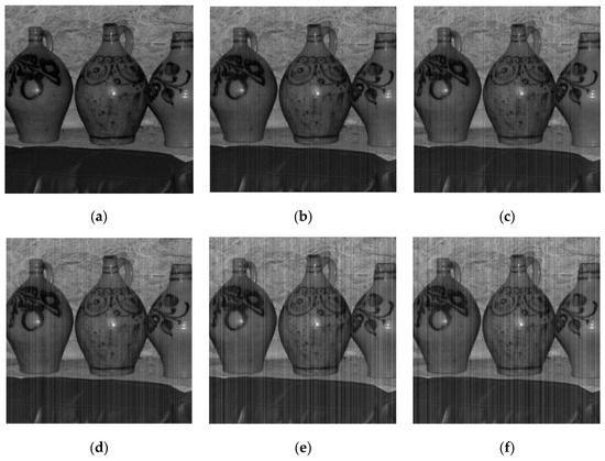
Figure 7.
Sets of simulated noisy images for ceramic. (a) Clean images; (b–f) Noisy images vase with stripe noise of = 0.03, 0.05, 0.08, 0.14, 0.20, respectively. The input image is available under the CC-BY license [28].
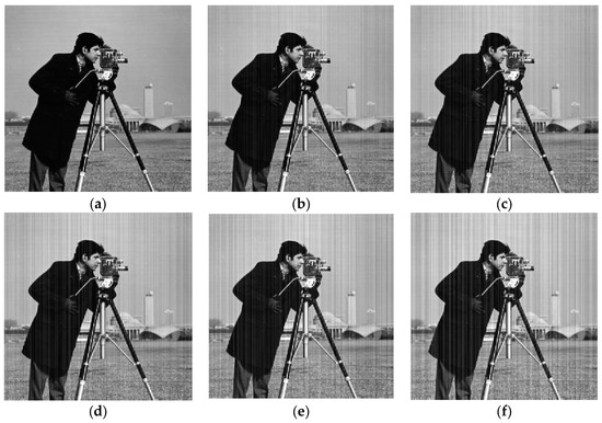
Figure 8.
Sets of simulated noisy images for cameraman. (a) Clean images people; (b–f) Noisy images people with stripe noise of = 0.03, 0.05, 0.08, 0.14, 0.20, respectively. The input image is available under the CC-BY license [28].
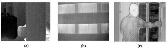
Figure 9.
Three raw infrared images for testing. (a) Suitcase from Tendero’s dataset [9]; (b) Leaves from Tendero’s dataset [9]; (c) People from Tendero’s dataset [9]. All of these images are available at the following link: http://demo.ipol.im/demo/glmt_mire/.

Table 1.
The details of the test data.
5.2. Analog Noise Image Test
In the simulation image test, two common image quality metric parameters are applied to evaluate the destriping performance, peak signal-to-noise ratio (PSNR) and structural similarity index (SSIM) of the algorithm [29]. PSNR can measures the pixel error between the output image and the reference image, and a higher PSNR value means a smaller degree of image distortion. The formula is defined as:
where MSE represents the mean square error between the output image and the reference image. SSIM provides the structural perception evaluation of filtering results within sliding window. The formula is defined as:
where m and n represents the image block extracted from the filtered image and the reference image by the sliding window, and , , , , represents the standard deviation, mean, and cross-correlation of m and n, respectively. and take constants to avoid the zero-denominator error in division. In experiment, the values of k1 and k2 are usually set to 6.5025 and 58.5225 [29]. In actual measurement results, the value of SSIM is usually between 0 and 1. The closer the SSIM value is to 1, the better the structure retention effect after image filtering.
Table 2 and Table 3 show the values of PSNR and SSIM for several methods respectively, which are obtained through 10 different noise processes. Compared with the three methods, it can be found that the PSNR value and SSIM value of the proposed method are the highest. It shows the superiority of this algorithm.
Table 2.
Peak signal to noise ratio (PSNR) (dB) results for ceramic and cameraman.
Table 3.
Structure similarity (SSIM) results for ceramic and cameraman.
To illustrate the advantages of the algorithm in this paper, an example is given as shown in Figure 10. It can be clearly seen that the raw image is contaminated by stripe noise with = 0.17. The results of CNN and TV processing by the algorithm also have obvious stripe noise. By contrast, the results obtained by MHE algorithm are better, but there will be an obvious “ghost” problem. Our proposed method achieves the best visual effect on the image, and the stripe noise is basically eliminated.
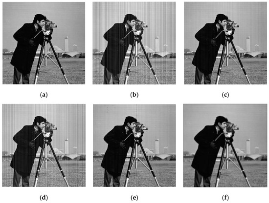
Figure 10.
Filtered results for cameraman corrupted by stripe noise with = 0.17. (a) Clean; (b) Noisy; (c) total variation algorithm (TV); (d) convolutional neural network (CNN); (e) midway histogram equalization algorithm (MHE); (f) Ours.
On the whole, our proposed method has achieved remarkable results in stripe correction through objective indexes and observation effects. In the next section, we will use the raw infrared image to evaluate the algorithm.
5.3. Infrared Image Test Evaluation
To better evaluate the denoising ability of the algorithm for infrared images, this section selects two major types of algorithms for comparison. One is the commonly used filtering algorithm (guided filtering with edge-preserving capability and commonly used smoothing filter), and the other is the current advanced stripe correction algorithm, namely, total variation algorithm (TV), midway histogram equalization algorithm (MHE) and CNN algorithm. Our proposed method is further evaluated through a comprehensive comparison.
5.3.1. Common Filtering Algorithm Evaluation
In this section, to verify the performance of our proposed algorithm, first of all, two common smoothing filters are applied to the infrared image. We selected infrared images with weak texture information and severe stripe noise [9]. The algorithm includes 1D Gaussian filtering and Guide filtering and then compare it with our proposed method.
We set the smoothing parameter of the 1D Gaussian filter to = 0.4, and the filtering window size of the 1D Gaussian filter to 3. Since the window value of the single guided filter is small, there will be a large amount of residual stripe noise, so the filter window for guided filtering is set to h = 0.5H and the regularization parameter is set to 0.22. For our own method, the wavelet basis function of wavelet decomposition is set as db1, the variance of vertical component column equalization is = 5, the regularization parameter of guided filter is set as 0.22, and the filtering window h is set as 0.3H. The comparison results are shown in Figure 11. It can be clearly seen that the Gaussian filter fails to distinguish the texture information from the noise, which reduces the gradient of the whole image and results in image blurring. Guided filter has a better effect of striping, but it can also blur the texture information. Our proposed method eliminates stripe noise while simultaneously retaining image details.
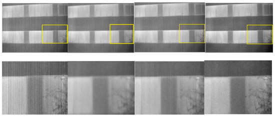
Figure 11.
Raw image Gaussian filtering Guided filtering Our method. Top: raw image and strip removal results using smooth filtering and our proposed method. Bottom: Zoom-in views of the highlighted region. Note that visually insignificant but important targets (e.g., trees and leaves) are smoothed out in the output of normal denoising algorithms. But in our results can still be easily identified. The input image is available under the CC-BY license [9]. Please zoom in to see details in the pictures.
5.3.2. Stripe Correction Algorithm Comparison Evaluation
Three sets of image sequences with different scenes and noises are used for the specific implementation. Corrected results for raw infrared image are shown in Figure 12, Figure 13 and Figure 14. Observing the image, it can be found that the processing effects of the four correction algorithms are obviously different. The correction results based on TV algorithm can protect the details and edge information of the image to the maximum extent, but many obvious vertical strips are still visible in the image (as shown in the red ellipse of the figure). The results obtained by MHE algorithm can better remove vertical strips but will over-smooth important details in infrared images. The results obtained by CNN algorithm have a good visual effect, but for the weak texture image, details will be lost (as shown in Figure 13). For our own method not only removes the stripe noise without introducing the ghost image, but also saves most of the edge details of the image.
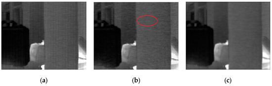
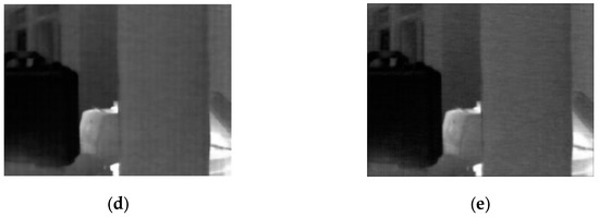
Figure 12.
Stripe non-uniformity correction results for suitcase. (a) Raw; (b) TV; (c) CNN; (d) MHE; (e) Ours. Please zoom in to see details in the pictures.
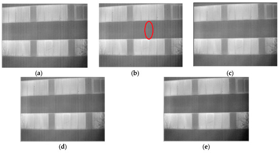
Figure 13.
Stripe non-uniformity correction results for leaves. (a) Raw; (b) TV; (c) CNN; (d) MHE; (e) Ours. Please zoom in to see details in the pictures.
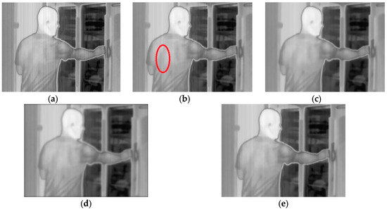
Figure 14.
Stripe non-uniformity correction results for people. (a) Raw; (b) TV; (c) CNN; (d) MHE; (e) Ours. Please zoom in to see details in the pictures.
To further prove the above point, we calculated the column mean of the raw image and the algorithm-corrected image. The result is shown in Figure 15. The effect of stripe noise can be regarded as the rapid change in the column mean. Figure 15a shows the change curve of the column mean value in Figure 14a. These changes are reduced after correction by the TV algorithm (Figure 15b), but some small fluctuations can still be observed, indicating residual non-uniformity without correction. MHE algorithm (Figure 15c) basically corrects these small fluctuations. However, the changes of image details are also lost, owing to being overly smooth. The proposed algorithm (Figure 15e) and CNN algorithm (Figure 15d) have similar results; small changes corresponding to image details are preserved, with stripe noise being simultaneously smoothed.
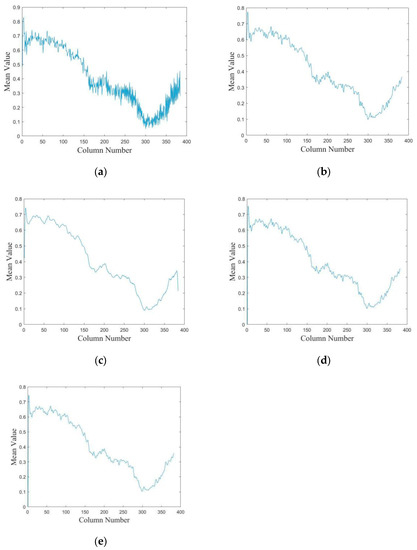
Figure 15.
Column mean transformation curves of original and corrected images. (a) Original image, (b) TV method, (c) MHE method, (d) CNN method, (e) Proposed method.
In addition to the visual contrast, we applied two objective indicators to evaluate the algorithm, image roughness index and average vertical gradient error (AVGE) [30].
The image roughness represents the richness of the image details. Its mathematical formula is as follows:
where h represents a differential filter; symbol represents a convolution operation; represents a first-order norm. The lower the value of , namely having low nonuniformity. Taking the raw infrared image and the simulated image (artificially add different intensity noise) as the samples to be processed through the TV, MHE, CNN and our proposed algorithm to obtain values in different scenarios. It can be found from Table 4 and Table 5 that the value of obtained by our proposed algorithm is the lowest, indicating that compared with the other image destriping algorithms, our proposed algorithm has an excellent ability to destripe noise.
Table 4.
ρ values of correction algorithms for raw infrared images.
Table 5.
ρ values of correction algorithms for simulated images.
To evaluate the detail protection ability of the algorithm, we introduce the value of AVGE to illustrate the detail protection ability of the algorithm. Its mathematical formula is as follows:
where is the noisy image with pixel p, is the denoising method, P is the number of pixels, and is the vertical gradient operator. AVGE represents the change of the gradient between the corrected image and the original image. The principle behind it is based on the understanding that stripe non-uniformity is reduced while the vertical gradient should remain unchanged. So, the AVGE value closer to 0 indicates that algorithm is better at preserving image detail. As can be seen from Table 6 and Table 7, CNN algorithm and the proposed algorithm get smaller AVGE values. However, as shown in Table 6, for the image of leaves with weak texture, CNN gives bad results. In fact, the CNN algorithm failed in this case. Overall, the experiment results reveal the advantage of the proposed method in stripe correction and detail preservation.
Table 6.
Average vertical gradient error (AVGE) values of correction algorithms for raw infrared images.
Table 7.
AVGE values of correction algorithms for simulated images.
5.4. Time Consumption
We considered the time consumption of different correction methods to examine their computation complexity. The experimental environment was Matlab 2016a, Intel core i5 CPU (3.40 GHz) and 8 GB RAM. We have calculated the running time of different methods for correcting infrared images. The statistical results are listed in Table 8. Compared with several other algorithms, the proposed method requires a minimum computing time. When the complexity of the scene increases, the time required for the proposed algorithm is basically stable at a very low level. This implies that our algorithm has the potential to be applied in hardware circuit systems.
Table 8.
Computing time (s) of different methods for simulated and raw infrared images.
5.5. Limitations of the Proposed Method
In this section, we added additional experiments to discuss the influence of a large amount of vertical edge information in the images on algorithms, such as radiator and fence scenes. Figure 16 shows an example for Fence, in which stripe noise with = 0.05 is added. The PSNR and SSIM results are shown in Table 9. From the results, we can see that our proposed method still has good ability to remove stripe in the scene with rich vertical information. In essence, stripe noise has its own characteristics. It can be seen that the intensity of each column of stripe noise is about the same, and the columns are significantly different between columns, and the shape is different from other types of noise. Therefore, noise can be effectively processed. However, it can also be seen from the correction image that the similarity between stripe and vertical edge will affect the correction result and produce artifacts, which is also our next research direction.
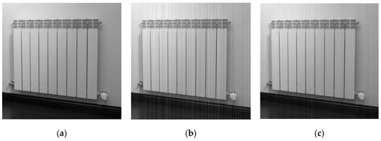
Figure 16.
Filtered result for Fence (a) Clean; (b) Noisy; (c) Corrected.
Table 9.
PSNR (dB) and SSIM results for Fence.
6. Conclusions
A stripe correction algorithm based on wavelet analysis and gradient equalization was proposed. Its advantage is that a Gaussian operator is introduced to perform a one-dimensional matrix convolution on the cumulative histogram of the vertical component and achieve gradient equalization in the horizontal direction. This ensures that no image details are lost in the denoising process. Compared with several algorithms with a better stripe effect, the experimental results show that the correction results of the proposed algorithm have better visual effects, and that the SSIM and PSNR indicators obtained by this algorithm are the best. It is shown that the proposed method can remove stripe noise and simultaneously preserve edge details.
Future work will focus on the spectral analysis of stripe noise; developing an adaptive stripe noise frequency detector is an interesting topic. Furthermore, additional prior knowledge of infrared images will be considered for stripe nonuniformity correction.
Author Contributions
All of the authors contributed to each facet of analysis and discussion and participated equally in the work of the paper.
Funding
This research received no external funding.
Conflicts of Interest
The authors declare no conflict of interest.
Abbreviations
The following abbreviations are used in this manuscript:
| FPN | Fixed Pattern Noise |
| FPA | Focal Plane Array |
| NUC | Non-Uniform Correction |
| CNN | Convolutional Neural Network |
| MHE | Midway Histogram Equalization |
| TV | Total Variation |
| PSNR | Peak Signal-to-Noise Ratio |
| SSIM | Structural Similarity |
| AVGE | Average Vertical Gradient Error |
References
- Cao, Y.; He, Z.; Yang, J.; Ye, X.; Cao, Y. A multi-scale non-uniformity correction method based on wavelet decomposition and guided filtering for uncooled long wave infrared camera. Signal Processing. Image Commun. 2018, 60, 13–21. [Google Scholar] [CrossRef]
- Zuo, C.; Chen, Q.; Gu, G.; Sui, X. Scene-based nonuniformity correction algorithm based on interframe registration. JOSA A 2011, 28, 1164–1176. [Google Scholar] [CrossRef] [PubMed]
- Sui, X.; Chen, Q.; Gu, G. Algorithm for eliminating stripe noise in infrared image. J. Infrared Millim. Waves 2012, 31, 106–112. [Google Scholar] [CrossRef]
- Cao, Y.; He, Z.; Yang, J.; Cao, Y. Spatially Adaptive Column Fixed-Pattern Noise Correction in Infrared Imaging System Using 1D Horizontal Differential Statistics. IEEE Photonics J. 2017, 9, 1–13. [Google Scholar] [CrossRef]
- Qian, W.; Chen, Q.; Gu, G.; Guan, Z. Correction method for stripe nonuniformity. Appl. Opt. 2010, 49, 1764–1773. [Google Scholar] [CrossRef] [PubMed]
- Friedenberg, A.; Goldblatt, I. Nonuniformity two-point linear correction errors in infrared focal plane arrays. Opt. Eng. 1998, 37, 1251–1253. [Google Scholar] [CrossRef]
- Harris, J.G.; Chiang, Y.M. Nonuniformity correction of infrared image sequences using the constant-statistics constraint. IEEE Trans. Image Process. 1999, 8, 1148–1151. [Google Scholar] [CrossRef] [PubMed]
- Pande-Chhetri, R.; Abd-Elrahman, A. De-striping hyperspectral imagery using wavelet transform and adaptive frequency domain filtering. ISPRS J. Photogramm. Remote Sens. 2011, 66, 620–636. [Google Scholar] [CrossRef]
- Tendero, Y.; Landeau, S.; Gilles, J. Non-uniformity correction of infrared images by midway equalization. Image Process. Line 2012, 2, 134–146. [Google Scholar] [CrossRef]
- Qian, W.; Chen, Q.; GU, G. Minimum mean square error method for stripe nonuniformity correction. Chin. Opt. Lett. 2011, 9, 34–36. [Google Scholar]
- Pipa, D.R.; da Silva, E.A.B.; Pagliari, C.L.; Diniz, P.S.R. Recursive algorithms for bias and gain nonuniformity correction in infrared videos. IEEE Trans. Image Process. 2012, 21, 4758–4769. [Google Scholar] [CrossRef]
- Maggioni, M.; Sanchez-Monge, E.; Foi, A. Joint removal of random and fixed-pattern noise through spatiotemporal video filtering. IEEE Trans. Image Process. 2014, 23, 4282–4296. [Google Scholar] [CrossRef]
- Hardie, R.C.; Hayat, M.M.; Armstrong, E.; Yasuda, B. Scene-based nonuniformity correction with video sequences and registration. Appl. Opt. 2000, 39, 1241–1250. [Google Scholar] [CrossRef]
- Cao, Y.; Yang, M.Y.; Tisse, C.L. Effective Strip Noise Removal for Low-Textured Infrared Images Based on 1-D Guided Filtering. IEEE Trans. Circuits Syst. Video Technol. 2016, 26, 2176–2188. [Google Scholar] [CrossRef]
- Liu, L.; Zhang, T. Optics temperature-dependent nonuniformity correction via L0-regularized prior for airborne infrared imaging systems. IEEE Photonics J. 2016, 8, 1–10. [Google Scholar]
- Tomasi, C.; Manduchi, R. Bilateral filtering for gray and color images. In Proceedings of the 6th International Conference on Computer Vision, Freiburg, Germany, 2–6 June 1998; pp. 839–846. [Google Scholar]
- He, K.; Sun, J.; Tang, X. Guided image filtering. In Computer Vision–ECCV; Springer: Berlin/Heidelberg, Germany, 2010; pp. 1–14. [Google Scholar]
- Kou, F.; Chen, W.; Wen, C.; Li, Z. Gradient domain guided image filtering. IEEE Trans. Image Process. 2015, 24, 4528–4539. [Google Scholar] [CrossRef]
- Tendero, Y.; Gilles, J. ADMIRE: A locally adaptive single-image, non-uniformity correction and denoising algorithm: Application to uncooled IR camera. In Infrared Technology and Applications XXXVIII, Proceedings of the SPIE Defense, Security, and Sensing, Baltimore, MD, USA, 23–27 April 2012; International Society for Optics and Photonics: Bellingham, WA, USA, 2012; p. 83531. [Google Scholar]
- Sui, X.; Chen, Q.; Gu, G. Adaptive grayscale adjustment-based stripe noise removal method of single image. Infrared Phys. Technol. 2013, 60, 121–128. [Google Scholar] [CrossRef]
- Boutemedjet, A.; Deng, C.; Zhao, B. Edge-aware unidirectional total variation model for stripe non-uniformity correction. Sensors 2018, 18, 1164. [Google Scholar] [CrossRef]
- Huang, Y.; He, C.; Fang, H.; Wang, X. Iteratively reweighted unidirectional variational model for stripe non-uniformity correction. Infrared Phys. Technol. 2016, 75, 107–116. [Google Scholar] [CrossRef]
- Kuang, X.; Sui, X.; Chen, Q.; Gu, G. Single Infrared Image Stripe Noise Removal Using Deep Convolutional Networks. IEEE Photonics J. 2017, 9, 1–13. [Google Scholar] [CrossRef]
- Li, H.; Manjunath, B.S.; Mitra, S.K. Multisensor image fusion using the wavelet transform. Graph. Models Image Process. 1995, 57, 235–245. [Google Scholar] [CrossRef]
- Zhu, Z.; Yin, H.; Chai, Y.; Li, Y.; Qi, G. A novel multi-modality image fusion method based on image decomposition and sparse representation. Inf. Sci. 2018, 432, 516–529. [Google Scholar] [CrossRef]
- Zhu, Z.; Qi, G.; Chai, Y.; Yin, H.; Sun, J. A novel visible-infrared image fusion framework for smart city. Int. J. Simul. Process Model. IJSPM 2018, 13, 144–155. [Google Scholar] [CrossRef]
- Liu, Z.; Xu, J.; Wang, X.; Nie, K. A fixed-pattern noise correction method based on gray value compensation for TDI CMOS image sensor. Sensors 2015, 15, 1764–1773. [Google Scholar] [CrossRef]
- He, K.; Sun, J.; Tang, X. Guided image filtering. IEEE Trans. Pattern Anal. 2013, 35, 1397–1409. [Google Scholar] [CrossRef]
- Wang, Z.; Bovik, A.C.; Sheikh, H.R.; Simoncelli, E.P. Image quality assesment: From error visibility to structural similarity. IEEE Trans. Image Process. 2004, 13, 600–612. [Google Scholar] [CrossRef]
- Zeng, Q.; Qin, H.; Yan, X.; Yang, S.; Yang, T. Single Infrared Image-Based Stripe Nonuniformity Correction via a Two-Stage Filtering Method. Sensors 2018, 18, 4299. [Google Scholar] [CrossRef]
© 2019 by the authors. Licensee MDPI, Basel, Switzerland. This article is an open access article distributed under the terms and conditions of the Creative Commons Attribution (CC BY) license (http://creativecommons.org/licenses/by/4.0/).