Deep Learning Based Computer Generated Face Identification Using Convolutional Neural Network

Abstract

Generative adversarial networks (GANs) describe an emerging generative model which has made impressive progress in the last few years in generating photorealistic facial images. As the result, it has become more and more difficult to differentiate between computer-generated and real face images, even with the human’s eyes. If the generated images are used with the intent to mislead and deceive readers, it would probably cause severe ethical, moral, and legal issues. Moreover, it is challenging to collect a dataset for computer-generated face identification that is large enough for research purposes because the number of realistic computer-generated images is still limited and scattered on the internet. Thus, a development of a novel decision support system for analyzing and detecting computer-generated face images generated by the GAN network is crucial. In this paper, we propose a customized convolutional neural network, namely CGFace, which is specifically designed for the computer-generated face detection task by customizing the number of convolutional layers, so it performs well in detecting computer-generated face images. After that, an imbalanced framework (IF-CGFace) is created by altering CGFace’s layer structure to adjust to the imbalanced data issue by extracting features from CGFace layers and use them to train AdaBoost and eXtreme Gradient Boosting (XGB). Next, we explain the process of generating a large computer-generated dataset based on the state-of-the-art PCGAN and BEGAN model. Then, various experiments are carried out to show that the proposed model with augmented input yields the highest accuracy at 98%. Finally, we provided comparative results by applying the proposed CNN architecture on images generated by other GAN researches.

1. Introduction

Over the past few years, the field of digital forensics has arisen to help restore some trust to digital images that appear all over the internet in an era of what is colloquially called “fake news”. Every day, vast amounts of multimedia content is generated through a variety of devices and shared via websites, magazines, newspapers, and television. Among them, image plays a crucial role regarding communication because it is considered one of the most influential communication media, which dominates most social network sites, mostly because existing mobile devices allow people to capture high-quality images anywhere at any time. Unfortunately, we cannot fully trust digital images as before. Given the advancement in computer vision in recent years, it has been easier to edit an image by using image processing and computer graphic techniques. Moreover, with the extensive availability of advanced image editing tools such as Adobe Photoshop and Gimp, altering a digital photo, with few signs or no visible sign of editing, has become more accessible and common. Generative adversarial networks (GANs), a class of artificial intelligence algorithms used in unsupervised learning, are emerging as a hot topic in the research community because of their ability to generate photographs that look at least superficially authentic to human observers, having many realistic characteristics. Some digital images generated by a GAN model are shown in Figure 1. Even after a close inspection, people may mistakenly identify a computer-generated image as original. The consequence would become even more severe if the images are used for commercial or political motives. As a result, there is an urgent need to develop a system which can verify an image’s authenticity. The verification process can be as simple as checking whether an image is generated by a computer (Classification), or as complicated as pointing out precisely which parts of the image are edited (Segmentation).

Figure 1. Example of computer-generated images generated by GAN (One of these is a photo of a real face, other faces are completely created by a GAN).

The images generated by GANs are becoming highly realistic [1,2]. However, each GAN model serves a specific topic in machine vision, and the generated images were varied in size and resolution. For any GAN, the optimal classifier belongs to its discriminator. Moreover, research focused on the detection of GAN-generated images has been limited. Thus, we propose a robust deep learning model which can detect images generated by multiple GAN models.

One of the biggest challenges GANs and other research topics have to deal with is the imbalance scenario, as the number of samples belonging to one class is much lower than those belonging to the other classes. There are different approaches to solving the imbalanced issue, such as resampling (i.e., trying to get an equal number of samples for both classes by increasing the frequency of the minority class and reducing the frequency of the majority class.), or ensemble (i.e., enhancing the classifier’s performance by building several two-stage classifiers from the original data and then adding up their predictions).

This paper proposes a system that can detect the face image generated by GAN networks. The main contributions of this work are as follows: (1) We propose a customized deep learning model (CGFace) that is specially designed for computer-generated detection task; (2) The boosting algorithms are applied on CGFace to detect computer-generated images efficiently (3) We implement two state-of the-art methods for generating computer-generated face images to create two huge datasets; and (4) Various experiments were conducted to examine the proposed model in (1) on the collected dataset in (2) to test the proposed model’s ability to detect images generated by different GAN models.

The rest of the paper is divided as follows. In Section 2, we thoroughly survey previous approaches to generative adversarial networks and computer-generated image problems. Some basic concepts are provided in Section 3. Next, the proposed CGFace and IF-CGFace frameworks will be explained carefully in Section 4. In Section 5, various experiments will be conducted to examine the effectiveness of the proposed model. Finally, in Section 6, we summarize and discuss future approaches.

2. Related work

2.1. Manipulated and Computer-Generated Face Image Detection Using CNN

Over the last ten years, computer vision has become universal in our society, with applications in image understanding, searching, mobile applications, medicine, mapping, drones, and autonomous driving cars. The backend to many of these applications is pattern recognition tasks such as localization, classification, and detection. Recent developments in deep learning algorithms have significantly improved the performance of these applications [3,4,5]. In the field of forensic image analysis, two common types of attacks are usually carried out: CG image (generated entirely by computer) and tampered image (parts of the image are altered).

For the problem of manipulated image detection, Bunk et al. [6] presented two methods to detect and localize manipulated regions in images: radon transform and deep learning. Experiments showed that both Convolutional Neural Networks (CNNs) and long short-term memory based networks were effective in exploiting resampling features to detect tampered regions. Bayar et al. [7] proposed a novel, CNN-based universal forgery detection technique that automatically suppressed an image’s content and learned important features for manipulation detection. The results of these experiments demonstrated that the proposed approach could automatically detect different types of manipulation with an average accuracy of 99.10%. Rao et al. [8] presented a customized CNN model, which was initialized with 30 primary high-pass filters for image steganalysis. The model’s architecture helped to efficiently suppress the effect of complex image contents and accelerate the convergence of the network. Extensive experiments demonstrated the superior performance of the proposed CNN-based scheme over other state-of-the-art image forgery detection methods. Salloum et al. [9] presented a technique that utilized a fully convolutional network (FCN) to localize image splicing attacks. They proposed the use of a multi-task FCN (MFCN) that used two output branches for multi-task learning. One branch was used to learn the surface label, while the other branch was used to learn the edge or boundary of the spliced region. Experiments showed that the SFCN and MFCN outperformed existing splicing localization algorithms concerning accuracy and testing time. Peng [10] proposed a novel network using both an RGB stream and a noise stream to learn rich features for image manipulation detection. The fusion of the two streams led to an improvement in performance. Experiments on standard datasets showed that their method not only detected tampering artifacts, but also distinguished between various tampering techniques. Han [11] suggested a two-stream tampered face detection technique, where one stream detected low-level inconsistencies between image patches, and another explicitly detected tampered faces; experimental results showed that this approach outperformed other methods because it was able to learn both tampering artifacts and hidden noise extra features.

For the task of computer-generated face image detection, Carvalho et al. in [1] took advantage of the inconsistencies of the eye’s region in CG images. They extracted the eye’s region features, with and without removing specular highlights, then applied transfer learning on VGG19. The proposed model achieved an AUC of 0.88 and an accuracy of 0.8. In video analysis, the problem of detecting computer-generated faces plays a vital role in identifying faces across frames of the video that have been taken using a different video recorder, or across time using a single camera. In 2018, Afchar et al. [12] provided two possible network architectures to detect forgeries efficiently with low computational cost. The experiments showed that their method had an average detection rate of 98% for Deepfake videos and 95% for Face2Face videos under real conditions of diffusion on the internet. In [13], a novel dataset of manipulated videos was proposed that exceeded all existing publicly-available forensic datasets by orders of magnitude. They also provided a benchmark for general image forensic tasks on this dataset such as identification and segmentation of forged images. Finally, they showed that handcrafted approaches were profoundly challenged by realistic amounts of compression, whereas they set a stable baseline of results for detecting a facial manipulation with modern deep learning architectures.

2.2. Generative Adversarial Networks (GANs)

Recently, several GAN-based methods have been proposed and have achieved great success in various computer vision related applications, such as image-to-image translation [14,15], super-resolution [16,17], image inpainting [18,19], and text to image [20,21,22]. For the image-to-image translation topic, Isola et al. in [14] investigated conditional adversarial networks for image-to-image translation problems, and they demonstrated that this approach was effective at synthesizing photos from label maps, reconstructing objects from edge maps, and colorizing images, among other tasks. Wang et al. [15] proposed a principled Perceptual Adversarial Networks (PAN) for image-to-image transformation tasks. The proposed PAN consisted of two feed-forward convolutional neural networks (CNNs): the image transformation network T and the discriminative network D. They achieved quite good image-to-image translation results. On the super-resolution topic, [16] presented a novel deep learning approach for single image super-resolution (SR). It was designed to learn the mapping between low and high-resolution images. Some extra pre-processing and post-processing were also conducted. It had a lightweight structure, yet demonstrated state-of-the-art restoration quality and achieved fast speed for practical on-line usage. Meanwhile, [17] described a deep residual network SRResNet that demonstrated a new state-of-the-art performance on public benchmark datasets when evaluated with the widely used PSNR measure. For image inpainting, Pathak in [18] presented Context Encoders—a convolutional neural network trained to generate the contents of an arbitrary image region conditioned on its surroundings. Through experiments, they found that a context encoder captured not just appearance but also the semantics of visual structures. Also, Li [19] proposed an effective face completion algorithm using a deep generative model; it was trained with a combination of a reconstruction loss, two adversarial losses and a semantic parsing loss, which ensured pixel faithfulness and local-global contents consistency. The results demonstrated qualitatively and quantitatively that the model was able to deal with a large area of missing pixels. Finally, in the text to image translation topic, Reed et al. in [21] presented the Generative Adversarial What-Where Network (GAWWN) that synthesized images given instructions describing what content to draw in which location. The model also enabled conditioning on arbitrary subsets of parts, and yielded an efficient interface for picking part locations. Zhang et al. [22] proposed Stacked Generative Adversarial Networks (StackGANs) aimed at generating high-resolution photo-realistic images. It included multiple generators and multiple discriminators arranged in a tree-like structure, that is, images at multiple scales corresponding to the same scene are generated from different branches of the tree. Extensive experiments demonstrated that the proposed stacked generative adversarial networks significantly outperformed other state-of-the-art methods in generating photo-realistic images.

One of the biggest challenges GANs and other research topics have to deal with is the imbalance scenario, as the number of samples belonging to one class is remarkably lower than those belonging to the other classes. There are different approaches to solving the imbalanced issue such as resampling (i.e., trying to get an equal number of samples for both classes by increasing the frequency of the minority class and reducing the frequency of the majority class.), or ensemble (enhancing the classifier’s performance by building several two-stage classifiers from the original data and then adding up their predictions).

For the task of generating CG image, GANs have achieved quite impressive performance because they can generate images that look realistic. Berthelot in [23] proposed a GAN architecture that effectively minimizes the Kullback-Leibler divergence between the real data distribution and the generated data distribution, and also changes the loss function by using auto-encoder as the discriminator. The experimental sections prove that its convergence is fast and stable, even in the absence of batch normalization, and that it generated and high visual quality. In the same year, Karas from NVIDIA [2] presented a new idea in training GAN model, and they tried to grow both the generator and discriminator consecutively by adding new layers that increased the fine details as training progressed. The construction of a higher-quality version of the CELEBA dataset proves that their method was very effective.

3. Preliminary

3.1. Generative Adversarial Network

The generative adversarial network (GAN) consists of a generator network $G$ and a discriminator network $D$. Given a training data $x$, the generator network $G$ adds a random noise $z$ and tries to generate data that has a similar distribution as the training data $x$. In contrast, discriminator network $D$ takes input from both the training data $x$ and the data generated by $G$, and it estimates the probability of a sample coming from training data rather than $G$.

To learn the generator’s distribution $p_z$ over the data $x$, the generator builds a mapping from a prior noise distribution $p_z\left(z\right)$ to data space as $G\left(z;{\theta }_g\right)$, where $G$ is a differentiable function represented by a multilayer perceptron with parameters ${\theta }_g$. Discriminator network $D$ is also represented as a multilayer perceptron $D\left(x;{\theta }_d\right)$, where ${\theta }_d$ is the parameters of the multiplayer perceptron.

$G$ and $D$ are trained simultaneously by adjusting parameters of $D$ to maximize the probability of assigning the correct label for both training examples and samples generated from $G$ and adjusting parameters of $G$ to minimize $\log \left(1-D\left(G\left(z\right)\right)\right)$. In other words, $D$ and $G$ play the following two-player minmax game with value function $V\left(G,D\right)$:

$$\underset{G}{\min }\underset{D}{\max }V\left(D,G\right)={\mathbb{E}}_{x~p_{data}\left(x\right)}\left[\log D\left(x\right)\right]+{\mathbb{E}}_{z~p_z\left(z\right)}\left[\log \left(1-D\left(G\left(z\right)\right)\right)\right]$$

(1)

Theoretically, when the adversarial process reaches the Nash equilibrium, the minmax game attains its global optimum. Since both sides want to undermine the others, a Nash equilibrium occurs when one player will not change its action regardless of what the opponent may do. Consider two players, $A$ and $B$, which control the value $x$ and $y,$ respectively. Player $A$ wants to maximize the value $xy$, while $B$ wants to minimize it.

$$\underset{B}{\min }\underset{A}{\max }V\left(D,G\right)=xy$$

(2)

The Nash equilibrium is when $x=y=0$. This is the only state where the action of the opponent does not matter. It is the only state that any opponents’ actions will not change the game’s outcome.

3.2. Imbalanced Scenario

From a practical viewpoint, the computer-generated face dataset is an imbalanced data scenario because the number of realistic computer-generated images is minor compared to real images. To reproduce this scenario, a new dataset is created which has a tiny number of computer-generated images, in contrast with the dominance of real images. $\partial$ represents the dataset and ${\partial }_m$ and ${\partial }_M$ indicate the minority class of the computer-generated images and the majority class of the real image, respectively. The dataset balancing ratio $r_{\partial }$ is computed as:

$$r_{\partial }=\frac{\left|{\partial }_m\right|}{\left|{\partial }_M\right|}$$

(3)

where $\left|.\right|$ represents the cardinality of a set. In the imbalanced scenario, the more severe the balancing ratio, the faster the accuracy drops of the minor class. The resampling technique turns $\partial$ into a new dataset ${\partial }_r$, such that $r_{\partial }>r_{{\partial }_r}$. On the other hand, the ensemble techniques have a different approach. Let’s consider the ensemble classifier in a binary classification; C(${\partial }_m$, ${\partial }_M$) is described as the cost of majority class samples being classified as minority class samples, whereas C(${\partial }_M$, ${\partial }_m$) indicates the cost of the remaining cases. The goal of the ensemble approach is to generate a model with the lowest misclassification cost, as described below:

$$Cost=C({\partial }_m,{\partial }_M)\times FN+C({\partial }_M,{\partial }_m)\times FP$$

(4)

where FP and FN are the numbers of false positive and false negative samples, respectively.

In the imbalanced class problem, special attention is needed on the accuracy of the correctly classified minor samples. For example, in the testing set, the real samples occupy 95% of the entire testing set, while computer-generated samples occupy only 5%. If the model predicted all samples belonging to the real class, the accuracy is considered to be 95%. In this case, we can mistakenly trust in the high performance of the system. That is the reason why the receiver operating characteristic (ROC) curve is widely used along with the accuracy, so that we are able to perceive the performance of the system thoroughly. To compare two or more models, the area under the ROC curve (AUC) is usually applied as the primary evaluation protocol for classification measurement. The higher the value of AUC, the better performance the model achieves.

4. Methodology

As depicted in Figure 2, we first introduce a customized deep learning model, namely CGFace model. Then, two state-of-the-art GAN models are implemented to create two datasets; one contains image generated by PCGAN [2], and the other contains images generated by BEGAN [23]. Before feeding generated datasets into CGFace model, we use the face detection module to extract the face and preprocessing this face. Finally, the processed datasets are used to examine the model performance.

Figure 2. Overall architecture of the proposed method.

4.1. The Proposed CGFace Model

In this section, we explain in detail our computer-generated face detection model called CGFace. To the best of our knowledge, little research has been done on detecting CG face images created by GAN models; take [2,23] as an example. Even though the two models were trained using the same CelebA, the generated images were completely different. Also, existing research on the topic [1,12] has mainly focused on monitoring the dataset, and then selecting and analyzing a set of representative features. Although the results were promising, these models were restricted to the selected features, so they will not work well on datasets that are slightly different from the training dataset. As the result, we propose a model which identifies computer-generated images created from different GAN models by automatically extracting characteristic features using the power of customized convolutional neuron network.

The first task is to select a suitable CNN architecture; this depends heavily on a practical point. By examining some state-of-the-art models [1,7,24] and comparing the performance, we discovered that five convolution layers were sufficient to handle the classification problem for the computer-generated face detection. After the number of convolution layers was decided upon, we examined the best kernel size to map the image input size to (1 × 2) output. Each layer must follow an appropriate kernel size to control the parameters’ flow. Figure 3 introduces each layer with its corresponding input, kernel, and output size. The input of this model is 64 × 64 grayscale images, while the output indicates whether the image is generated by a computer or by normal means. Overall, the proposed model contains five convolutional layers (Conv1 to Conv5), three max-pooling layers (Max-Pool1 to Max-Pool3) followed by a flattening and two fully connected layers or dense layers. As shown in Figure 3, the first convolutional layer (Conv1) filters the input image (64 × 64) using eight 5 × 5 learnable kernels. Next, the second convolutional layer (Conv2) filters eight 60 × 60 output feature maps from Conv1 with eight 5 × 5 kernels. Then, the third convolutional layer (Conv3) filters sixteen 28 × 28 output feature maps from max pooling layer (Max-pool1) with sixteen 3 × 3 kernels. The following fourth convolutional layer (Conv4) filters sixteen 13 × 13 output feature maps from the second max pooling layer (Max-pool2) with thirty-two 3 × 3 kernels. Finally, the final convolutional layer (Conv5) filters thirty-two 5 × 5 output feature maps from the third max polling layer (Max-pool3) with sixty-four 3 × 3 kernels. The sixty-four 3 × 3 output feature maps will be passed to flatten layer to give 576 values. Finally, the output layer only gives two classes, i.e., computer-generated and real.

Figure 3. CGFace model with detailed configuration for each layer.

The convolutional layer is the first layer of CNN used to extract features from an input image. Convolution preserves the relationship between pixels by learning image features using small squares of input data. Generally, increasing the number of convolutional layers will increase the learned feature complexity. The convolutional layer uses a set of learnable kernels sliding across the input image to extract the features. The convolution operation is illustrated as

$$x_j^l=f\left({{\displaystyle \sum }}_{i\in {\Omega }_j}{x}_i^{l-1}\ast k_{ij}^l+b_j^l\right)$$

(5)

where $x_j^l$ is the $j$-th output feature map of layer $l$ and $x_i^{l-1}$ is the $i$-th input feature map of the previous layer $\left(l-1\right)$ of layer $l$. ${\Omega }_j$ indicates a set of input feature maps. $b_j^l$ is the bias and $k_{ij}^l$ kernel connects the $i$-th and $j$-th feature maps. Finally, the activation function $f(·)$ conducts a nonlinear transformation. In the presented model, rectified linear unit (ReLU) nonlinearity function ($f=\max \left(0,x\right)$) was applied on the activation layer because it was shown to have higher fitting abilities than a hyperbolic or sigmoid function [25].

The pooling layer is commonly placed after the convolutional layer to reduce the number of parameters and prevent the overfitting problem. It is fed a small square block ($s\times s)$ from the output feature map of the convolutional layer. Then, for each block, an algorithm is applied to reduce the parameters and produces a single output. The most popular pooling method is average pooling or max pooling. We implement the max-pooling in our model; it is calculated as follows:

$$y_{j,k}^i={\max }_{0\le m,n\le s}\left\{x_{j·s+m,k·s+n}^i\right\}$$

(6)

where the feature map of the previous convolutional layer is $i$, and the equation takes the $s\times s$ region and produces a single value. It reduces the $N\times N$ input map to the $\frac{N}{s}\times \frac{N}{s}$ output map.

After a chain of convolution and pooling layers, the last output is a one-by-two vector (one is “computer generated” and the other is “real” class). Each neuron from the output layer fully connects to the features map from the previous hidden layer. Let $x$ indicate the last hidden layer output, while $w$ stands for the weights between the final hidden layer and the output layer. The output is defined as $f=w^{T}x+b$. It is fed into a softmax classifier which produces a probability distribution for the two class labels:

$$O_k=\frac{\exp \left(f_x\right)}{{{\displaystyle \sum }}_{j=1}^2\exp \left(f_j\right)}$$

(7)

where $O_k$ is the probability of the $k$-th class and ${\displaystyle \sum }_{k=1}^2{O}_k=1$. In our work, we used Keras library—an open source deep learning framework written in Python to construct and train the model.

4.1.1. Dropout Layer

As explained in [24], to improve the model performance, the depth of hidden layers must be increased notwithstanding the fact that increasing the depth makes the model less and less stable. The instability, in this case, means overfitting during the training. Dropout is a regularization method used to prevent overfitting while training neural nets; it turns-off some of the hidden units (with some probability) so that they do not learn every unnecessary details of instances in the training set. This mechanism injects noise into the network to force it to learn to generalize well enough to deal with noise. Table 1 shows the configuration and location of the dropout layers in the CGFace model. The dropout rate was set to 0.2 across all the dropout layers.

Table 1. Layer breakdown for the proposed CGFace model.

Layer	Configuration	Output (Rows, Cols, Channels)
Input	64 × 64
Convolution_1	5 × 5 with 8 kernels	(60, 60, 8)
Convolution_2	5 × 5 with 8 kernels	(56, 56, 8)
Maxpool_1	2 × 2	(28, 28, 8)
Dropout_1	Probability at 0.2	(28, 28, 8)
Convolution_3	3 × 3 with 16 kernels	(26, 26, 16)
Maxpool_2	2 × 2	(13, 13, 16)
Dropout_2	Probability at 0.2	(13, 13, 16)
Convolution_4	3 × 3 with 16 kernels	(11, 11, 32)
Maxpool_3	2 × 2	(5, 5, 32)
Dropout_3	Probability at 0.2	(5, 5, 32)
Convolution_5	3 × 3 with 16 kernels	(3, 3, 64)
Dropout_4	Probability at 0.2	(3, 3, 64)
Flatten	Length: 576	(576)
Dense	Length: 256	(256)
Dense	Length: 2	(2)

4.1.2. Batch Normalization

In the proposed model, before the fully connected layers, one batch normalization layer was added. The purpose of this layer is to improve optimization by introducing some noise into the network so that it can regularize the model besides the dropout layers a little bit more. It normalizes the input $x$ from the preceding layer by deducting the batch mean and dividing it to batch standard deviation. The result is squashed through a linear function with parameters called “standard deviation” ($\gamma$) and “mean” ($\beta$). If $\gamma =\left(var\left(x\right)\right)$ and $\beta =mean\left(x\right)$, the original activation is restored. The equation is what makes batch normalization robust. Initially, batch normalization is set to convert the input to zero means. However, during the training process, it can learn from any other distribution. Batch normalization enables each layer to learn by itself. The detailed description of the algorithm is shown in [26].

4.1.3. Adam Optimization

Adam (adaptive moment estimation) [25] is an optimization algorithm that replaces the classical stochastic gradient descent procedure to update the network weights. Besides storing an exponentially-decaying average of the past squared gradients $v_t$, Adam also keeps an exponentially-decaying average of past gradients $m_t$, similar to momentum.

The decaying averages of past ($d_t$) and past squared gradients ($p_t$) at timestep $t$ are computed as follows:

$$d_t={\beta }_1{m}_{t-1}+\left(1-{\beta }_1\right)g_t$$

(8)

$$p_t={\beta }_2{v}_{t-1}+\left(1-{\beta }_2\right)g_t^2$$

(9)

Let $d_t$ and $p_t$ be the estimation of the first moment (the mean), and the second moment (the un-centered variance) of the gradients respectively, and $g_t$ be the gradient of the stochastic objective, $g_t^2$ (indicates the elementwise square $g_t\odot g_t$) a function of the gradients at all previous time steps. $d_t$ and $p_t$ were initialized as vectors of 0’s, the authors in [25] noticed that they were biased towards zero, mainly during the initial time steps, and when ${\beta }_1$ and ${\beta }_2$ were close to 1 (the decay rates are small). The parameters β₁ and β₂ do not precisely define the learning rate, they decay the running average of the gradient. If they decay rapidly, then the learning rates will jump about all over the place. If they decay slowly, it will take ages for the learning rates to be learned.

To prevent this problem, bias-corrected first (${\widehat{d}}_t$) and second moment (${\widehat{p}}_t$) estimates are calculated:

$${\widehat{d}}_t=\frac{d_t}{1-{\beta }_1^t}$$

(10)

$${\widehat{p}}_t=\frac{p_t}{1-{\beta }_2^t}$$

(11)

Bias-corrected first and second-moment estimations are then used to update the parameters, which yield the Adam update rule, $\eta$ indicates the step size parameter:

$${\theta }_{t+1}={\theta }_t-\frac{\eta }{\sqrt{{\widehat{p}}_t}+ϵ}{\widehat{d}}_t$$

(12)

4.2. Gradient Boosting for the Imbalanced Data Problem

Gradient boosting is a learning algorithm explicitly designed for classification and regression situations, which generates a model as a collection of weak prediction models (decision trees). It starts with a simple decision tree. After the tree has been trained, a list of samples for which the tree makes classification mistakes is recorded. After that, a second tree is trained to predict how wrong the other tree classified an input and tried to correct the predictions of the first tree. Next, another tree is constructed that again tries to estimate the error of its other tree, and so on.

Extreme gradient boosting (XGBoost) is among the most famous algorithms in supervised learning these days, and one of the most well-known implementations of the gradient boosting concept. It was proposed by Chen and Guestrin [27]. The robustness and speed of the algorithm was fast compared to other gradient boosting implementations.

$$Obj=L+\Omega$$

(13)

where $L$ is the loss function which controls the predictive power, and $\Omega$ is the regularization component which controls simplicity and overfitting. The loss function $L$ which needs to be optimized can be Root Mean Squared Error for regression, Log loss for binary classification, or mlogloss for multi-class classification. The regularization component $\Omega$ is dependent on the number of leaves and the prediction score assigned to the leaves in the tree ensemble model.

Moreover, Adaptive Boosting, short for AdaBoost [28], which is another great machine learning algorithm, is also used to learn the features extracted from the MANFA model. Given a training set $TS=\left(x_1,y_1\right)\dots \left(x_m,y_m\right)$, where $x_i\in X,y_i\in Y=\left\{-1,+1\right\}$, it tries to preserve a distribution or a set of weights over the training set. AdaBoost first tries to find a weak hypothesis $X\to \left(-1,+1\right)$. The last output is based on the majority vote of all the weak hypotheses:

$$H\left(x\right)=sgn\left({{\displaystyle \sum }}_{t=1}^T{\alpha }_t{\mathrm{h}}_t\right)$$

(14)

where $T$ is the total number of the weak hypotheses and ${\alpha }_t$ is the weight assigned to ${\mathrm{h}}_t$.

4.3. Detailed Implementation of the Two Dataset

As described at the beginning of Section 4, we reimplemented two state-of-the-art GAN models to gather two datasets for the evaluation of the proposed model. The first dataset is generated using PCGAN’s pre-trained model [2]. In PCGAN, the authors started with small generator and discriminator networks trained on low-resolution images. Then, step by step, they added in additional layers and trained with increasingly higher resolution images. In contrast, the second dataset was created by using Boundary Equilibrium Generative Adversarial Networks (BEGAN) proposed by [23] to generate computer-generated images based on the CelebA dataset. BEGAN is a state-of-the-art architecture when it comes to generating realistic faces. The primary goal behind the BEGAN is to change the loss function, and it is achieved by making $D$ an autoencoder. The loss is a function that decides the quality of reconstruction achieved by $D$ on real and generated images.

Another advantage of BEGAN is that it is usually tricky (and zero-sum game) to show that the GANs model converged, and BEGAN brings the concept of equilibrium to present a global measure of convergence.

4.3.1. Equilibrium

The reconstruction losses are considered to be at equilibrium when the distributions of the reconstruction losses of real $ℒ\left(\mathrm{x}\right)$ and generated images $ℒ\left(\mathrm{G}\left(\mathrm{z}\right)\right)$ are equal:

$$\mathbb{E}\left[ℒ\left(\mathrm{x}\right)\right]=\mathbb{E}\left[ℒ\left(\mathrm{G}\left(\mathrm{z}\right)\right)\right]$$

(15)

If equilibrium were reached, it would mean that $D$ becomes incapable distinguishing generated samples from real ones. For the training to go smoothly, neither network should win over the other, so the strategy is to define a ratio $\gamma$ between the two losses.

$$\gamma =\frac{\mathbb{E}\left[ℒ\left(G\left(z\right)\right)\right]}{\mathbb{E}\left[ℒ\left(x\right)\right]}$$

(16)

$\gamma$ is called the diversity ratio, and it should be either [0,1]. Lower values of $\gamma$ lead to $\mathbb{E}\left[ℒ\left(x\right)\right]\gg \mathbb{E}\left[ℒ\left(\mathrm{G}\left(\mathrm{z}\right)\right)\right]$, which means $D$ focuses more on its auto-encoding task, and $G$ has an incentive to produce more realistic images, which may be at the cost of image diversity. On the other hand, a higher value of $\gamma$ leads to $\mathbb{E}\left[ℒ\left(x\right)\right]=\mathbb{E}\left[ℒ\left(\mathrm{G}\left(\mathrm{z}\right)\right)\right]$ which means that $D$ focuses more on its discrimination task, and $G$ has an incentive to produce more realistic images, which may be at the cost of image diversity.

Figure 4 from [23] shows the differences of the generated images when the hyperparameter $\gamma$ is set to different value. Overall, the model worked well when the value is changed because it still maintains a degree of face diversity across the range of $\gamma$ values. At low value (0.3), the generated faces look generally uniform. However, at the higher value of $\gamma$, e.g., 0.7, the variety of the generated faces increase, but artifacts and noise also appear more frequently.

Figure 4. Generated images with different values of the hyper parameter $\gamma$ (some noise-like regions are marked with red).

4.3.2. Balancing the Losses

To maintain the ratio $\gamma$ between the two reconstruction losses over time, the author [23] added an adaptive term $k_t\in \left[0,1\right]$ to control this ratio dynamically during the training.

$$\{\begin{array}{c}{ℒ}_D=ℒ\left(x\right)-k_tℒ\left(G\left(z\right)\right)\\ {ℒ}_G=ℒ\left(G\left(z\right)\right)\\ k_{t+1}=k_t+\lambda \ast (\gamma .ℒ\left(x\right)-ℒ\left(G\left(z\right)\right)\end{array}$$

(17)

with $\lambda$ being the learning rate that adapts $k_t$ over time is also called the proportional gain for k and in practice, it is set to 0.001.

4.3.3. Convergence Measure

The convergence of BEGAN was fast and stable because it has to satisfy two main points:

• $ℒ\left(\mathrm{x}\right)$ should go to 0 as images are reconstructed better and better after each time step.
• $\gamma .ℒ\left(x\right)-ℒ(G\left(z\right)$) should stay close to 0 (so that the losses are balanced).

The combination of these two points implies that $ℒ(G\left(z\right)$) goes to 0 and that $\mathcal{P}(G\left(z\right))$ get closer to ${\mathcal{P}}_x$. If we add (a) & (b) up, we will get the following convergence measure:

$${\mathrm{M}}_{global}=ℒ\left(\mathrm{x}\right)+\left|\gamma .ℒ\left(x\right)-ℒ\left(G\left(z\right)\right)\right|$$

(18)

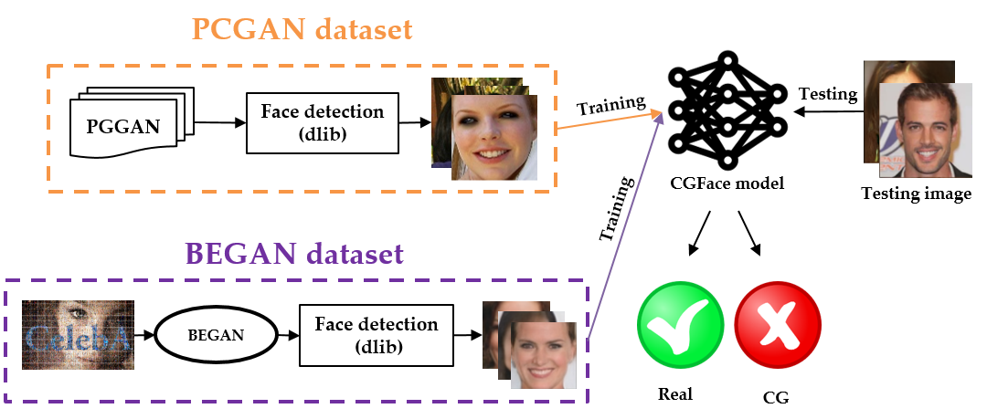
4.4. Face Detection Module

After the two datasets were collected, a face detection module was conducted using facial landmarks [29]. They have been successfully applied to head pose estimation, face alignment, blink detection, and face swapping. Facial landmarks can localize the face in the image as well as detect the key facial structures on the face such as the eyes, mouth, and nose. However, in this research, we only applied them to detect the face; we used the C++ dlib toolkit (https://github.com/davisking/dlib), which contains a pre-trained HOG (Histogram of Oriented Gradients) and Linear SVM object detector to detect the face in the image.

5. Experimental Results

5.1. Evaluation Metric: ROC Curve

In binomial classification, the results can be depicted by a confusion matrix, as shown in Table 2. Two important evaluation metrics based on the confusion matrix, including true positives rate (TPR) or sensitivity and false positives rate (FPR) or 100-Specificity, are defined as below:

$$\begin{gathered} TPR=\frac{TP}{TP+FN} \\ FPR=\frac{FP}{FP+TN} \end{gathered}$$

(19)

where TP, FN, FP, and TN are described in Table 2. In the ROC curve [30], the TPR is plotted in function of the FPR (100-Specificity) for different cut-off points. Each point on the ROC curve represents a sensitivity/specificity pair corresponding to a particular decision threshold.

Table 2. A confusion matrix for summarizing the classification results.

		Prediction
		Normal	CG
Actual	Normal	TP (True positive)	FN (False negative)
	CG	FP (False positive)	TN (True negative)

To compare two classifiers using ROC curve (for example M1 and M2), AUC [30], the area under the ROC curve is used. If ROC curve M1 occupies a larger AUC than ROC curve M2, then the M1’s classifier is considered to achieve better performance compared to the M2’s classifier.

5.2. Dataset

Both PCGAN and BEGAN used CelebA as a training dataset. It contains approximately 202,600 celebrity face images [31] and has a huge variety of facial poses, including rotations around the camera axis. There are two sub data in the dataset, “In the wild” and “Align and cropped”. The “In the wild” dataset is varied and potentially harder to model than the “Align and cropped” dataset, presenting an interesting challenge. We prefer to use “Align and cropped”, since the main study interest is identifying images generated by artificial intelligence.

Section 5.2.1 and Section 5.2.2 show the number of images in BEGAN and PCGAN, respectively.

5.2.1. PCGAN

In our experiments, we randomly selected 5000 real face images from CelebA dataset and 5000 fake ones of good quality from the fake face image database (https://goo.gl/ozy7Kq) shared by [2]. All collected images were in 256 × 256 and stored in PNG format. In our experiments, we resized all images into 64 × 64 using bilinear interpolation and compressed them using lossy JPEG compression with a quality factor of 95. Finally, we divided the images into the training set (3750 pairs of true-fake face images), the validation set (1250 pairs). To achieve convincing results, we used four-fold cross-validation and reported the average results in the following experiments.

5.2.2. BEGAN

For the BEGAN model proposed by [23], the author did not share their dataset, so we implemented their proposed method and tried to generate computer-generated images based on the CelebA dataset as previously described in Section 4.3. The BEGAN is a generative adversarial network (GAN) which applies an auto-encoder as the discriminator. The authors also used an equilibrium method for balancing adversarial networks which helped the network converged to diverse and visually pleasing images.

For the balance between D and G—gamma is set to 0.4, the total number of iterations is 200,000, the batch size is 16, the BEGAN’s learning rate is set to 0.0001, while the learning rate of k is set to 0.001, the learning rate will be decayed after 3000 iterations.

Figure 5 describes the results after different iterations. It is easy to notice that at the beginning of the training process (iteration 5000), the generated images are blurry; however, at the end of the training process (iteration 200,000), the generated images become more realistic.

Figure 5. Differences in the generated images when the number of iterations increases.

The total training time is approximately 6 h; each epoch takes an average of 9 s. Then the trained model was used to generate 5000 computer-generated images of size 64 × 64. Figure 6 shows some samples of the dataset. Some of the generated images look realistic, such as the images in row 8, column 8 and row 7, column 2.

Figure 6. Images with the size of 64 × 64 generated by the BEGAN model.

5.3. Evaluation of the CGFace Model

First of all, we examined the performance of CGFace on two generated datasets. For PCGAN, the original size 256 × 256 of the input image is resized to 64 × 64. After that, the faces are detected, rotated, and aligned to frontal using dlib library to eliminate the pose changes. After that, four-fold cross-validation is conducted; it randomly divides the data into four subsets, in which each subset contains 5000 images. Each time, three subsets are fed into the model to train the proposed CNN, while the other subset used for testing purpose. Then, for the training set, 75% of the training data is used by the convolutional neural model to learn and update the weight, whereas the remaining 25% is used to validate data to fine-tune the parameters. The complete validation accuracy and loss for each fold are given in Figure 7. The optimization algorithm used in CGFace is Adam optimization [25] with a learning rate of 0.001, a batch size of 32, and 50 epochs.

Figure 7. Generated images from the trained PCGAN model.

As shown in Figure 7, the training/validation accuracy increases dramatically to over 80%, while the training/validation loss drops significantly to under 30% after the first few epochs. For the rest of the training process, the training/validation accuracy gradually increases and reaches a peak at nearly 98%. In contrast, the training/validation loss slowly decreases and hits bottom at 3%. Among four folds, fold four yields the best results regarding validation accuracy and validation loss as well as the model stabilization. Fold 4 yields the best results because the model in fold 4 is well trained without the overfitting problem. On the other hand, the other folds have fluctuations in the training loss and validation loss.

Next, we performed a similar process as the PCGAN’s experiment for the BEGAN dataset. As shown in Figure 8, the training/validation accuracy leaps to over 90%, whereas the training/validation loss plummets to 10% after the third epoch. For the rest of the training process, the training/validation accuracy gradually increases and reaches a peak at nearly 97%. In contrast, the training loss and validation loss slowly decreases and hits bottom at 3%. Within four folds, fold three yields the best results concerning validation accuracy and validation loss as well as the model stabilization.

Figure 8. Generated images from the trained BGAN model.

5.4. Evaluation of the CGFace, IF-CGFace Model on the PCGAN Dataset

Through the previous experiments, the proposed CGFace was shown to perform well with images generated by different kind of GAN models. However, the performance of CGFace and IF-CGFace (which includes XGB-CGFace and ADA-CGFace) should be compared under the same environment, so the last dense layer was removed from the CG-Face and replaced by XGB or AdaBoost to examine the performance of IF-CGFace. We will use PCGAN dataset for the following experiments because the images generated from PCGAN were more realistic compared to BEGAN.

5.4.1. Balanced Scenario

Firstly, the output feature map was extracted from the last hidden layer of the model of the fold 4 (PCGAN) from previous experiment. Next, the softmax classifier was replaced by the AdaBoost and XGB classifiers. The performance results of our CGFace model compared with ADA-CGFace, XGB-CGFace, and VGG16 (different classifiers and feature types) are shown in Table 3. We quickly notice that the CGFace model achieves 98% accuracy, whereas the AUC is only 81%. In contrast, although the classification accuracy of IF-CGFace models is similar to that of CGFace, XGB-CGFace yields AUC at 84.2%, while ADA-CGFace achieves 89.4%, outperforming CGFace. The result suggests that batch normalization and dropout layers which were placed after each convolution layer can reduce not only overfitting data during training, but also increase the performance of computer-generated face detection.

Table 3. The performance summarization of different models on PCGAN dataset.

Model	Classifier	Accuracy (%)	AUC
VGG16	Softmax	76	80.5
CGFace	Softmax	98	81
ADA-CGFace	AdaBoost	97.3	89.4
XGB-CGFace	XGB	92.6	84.2

5.4.2. Imbalanced Scenario

In the imbalanced experiment, a new dataset is created from PCGAN dataset with the balancing ratio of 1/10 indicating that the number of real images are 10 times more than the number of computer-generated images (the real class contains 1000 images, whereas the computer-generated class contains only 100 images). After that, 4-fold cross-validation is conducted on three different models: the CGFace model and IF-CGFace models (including AdaBoost and XGB). We follow the transfer learning procedure in deep learning for imbalanced dataset by extracting output features map from the hidden layer before the final dense layer. Then, the features are trained in AdaBoost classifier to form ADA-CGFace model and XGB classifier to form XGB-CGFace. As we can observe in Figure 9, in the most imbalanced case, in which the number of computer-generated images is a minority compared to the majority of real images, the CGFace model gets the lowest AUC, which also means that it worked poorly on the imbalance scenario because it misclassified many CG images. In contrast, for fold 4, IF-CGFace, and especially ADA-CGFace performed well at 90.1% AUC. The results prove the effectiveness of AdaBoost and XGB classifiers on the imbalanced environment.

Figure 9. A comparison regarding AUC for various methods through 4 folds on the imbalanced environment (No. CG images / No. real images = 1/10).

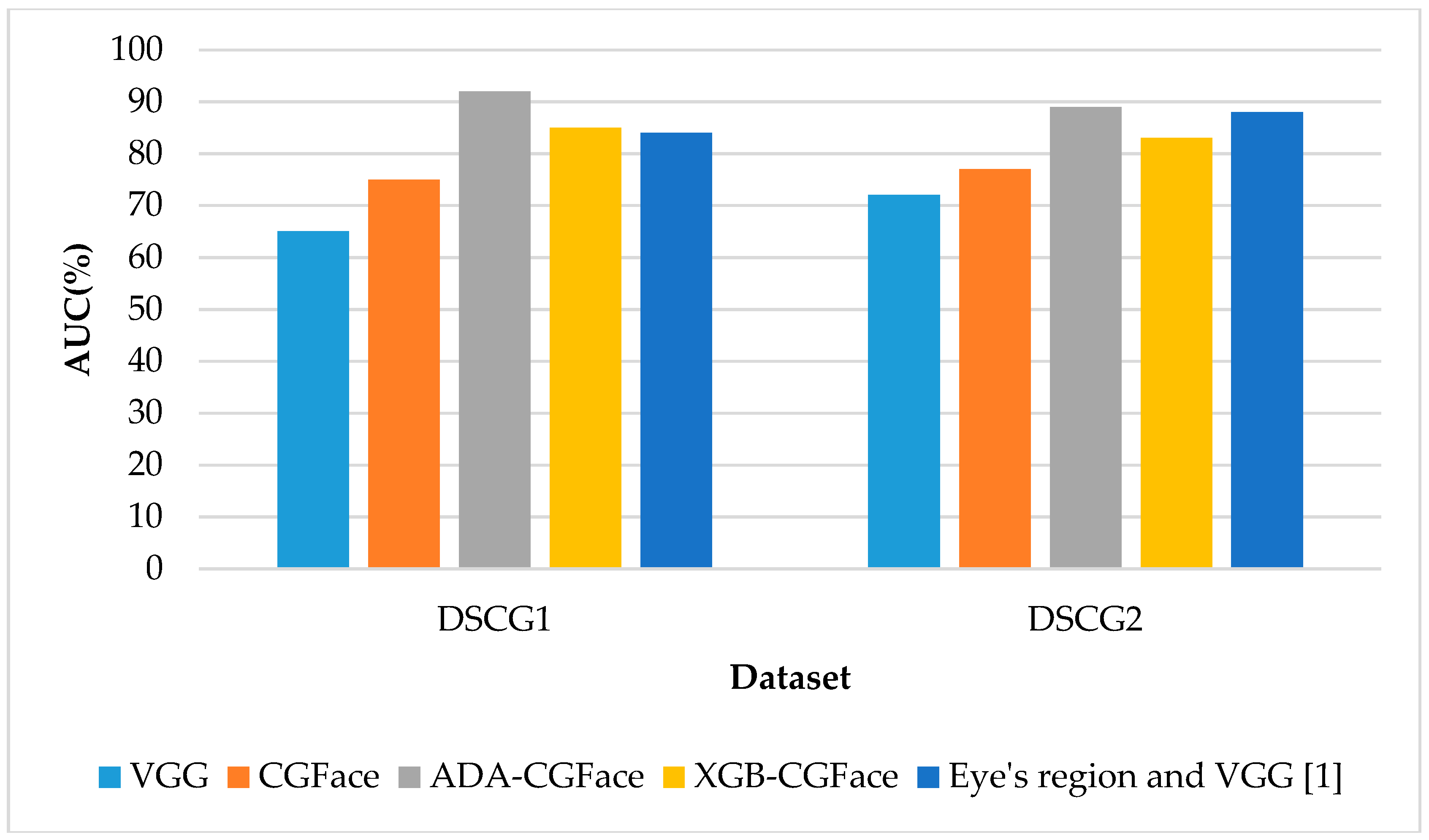
5.5. Compare the Model Performance with Recent Researches

In the second experiment, we used AUC values to compare the performance of CGFace, IF-CGFace with VGG and its performance on DSCG1 and DSCG2 computer-generated dataset [1].

For the VGG-16 implementation, we used the default configuration, i.e., image size of 224 × 244, learning rate 0.01, and 30 epochs. For the work in [1], The first dataset (DSCG1) composed of 30 extremely realistic CG images of faces collected from different websites and 30 PG images. The 30 CG images depict 15 male and 15 female faces with image resolutions varying from 389 × 600 to 557 × 600 pixels. PG images have resolutions varying from 387 × 600 to 594 × 600 pixels. The second dataset (DSCG2) composed of 160 images (80 CG and 80 PG) with the resolution from 236 × 308 to 1569 × 2000 for CG images and from 194 × 259 to 5616 × 3744 for PG images. The author in [1] proposed a new CG image detection method that took advantage of the inconsistencies occurring in eye’s region of CG images containing people. Given an image of a person, they extracted features from eye’s region with and without removing specular highlights, using a deep convolutional neural network model based on VGG19 and transfer learning approach.

As shown in Figure 10, our ADA-CGFace outperforms VGG as well as the model proposed by [1] on DSCG1 and DSCG2 dataset. The highest AUC achieved on ADA-CGFace is on DSCG1 dataset, at about 92%, followed by XGB-CGFace at 85% on DSCG2 dataset. On DSCG1 and DSCG2, the reported AUC [1] were 84% and 88%, respectively, whereas our model achieved an AUC of 92% for DSCG1 and 89% for DSCG2.

Figure 10. The AUC performance of the proposed models and two other models on different datasets.

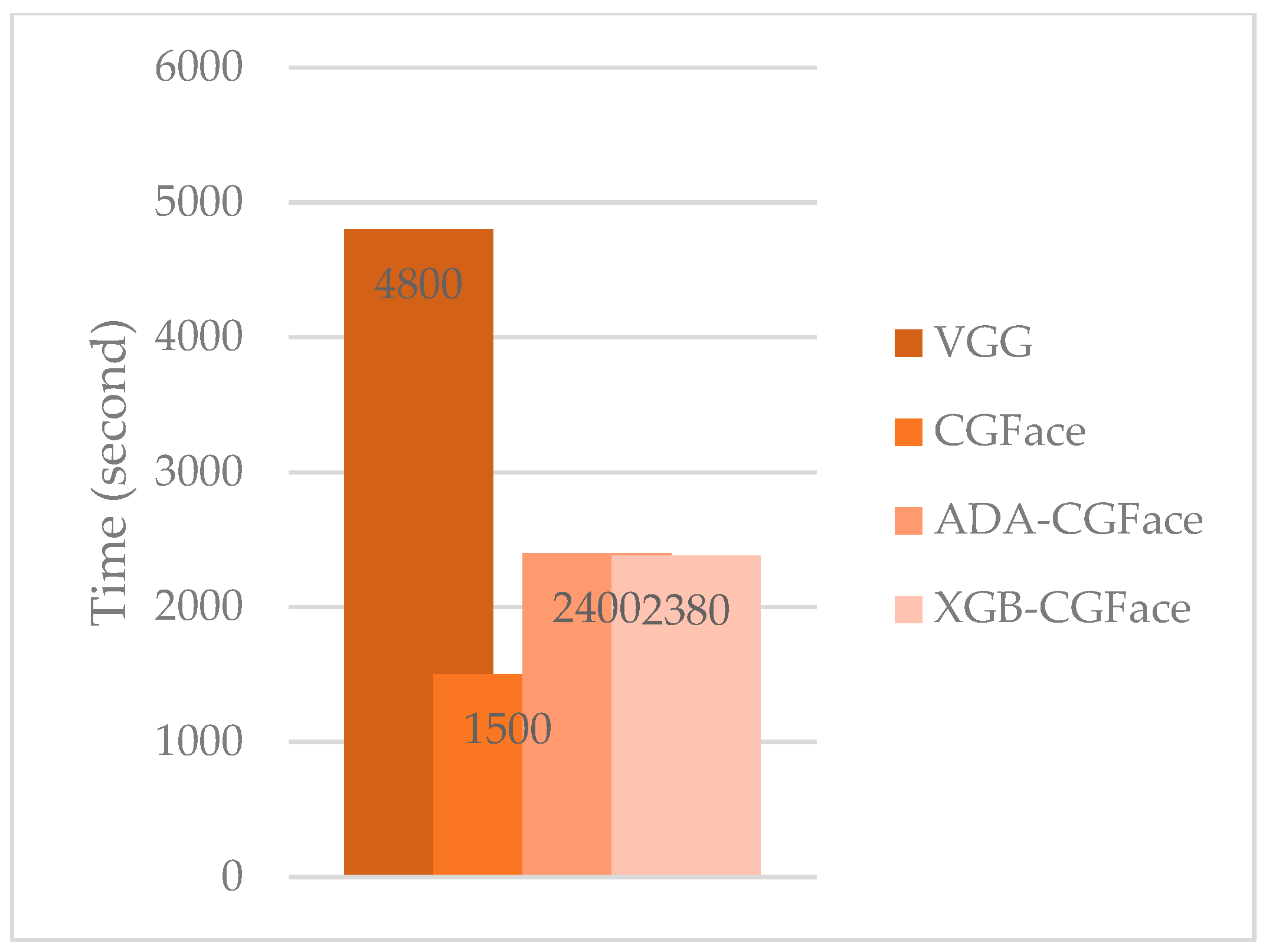
5.6. Training and Validation Time Analysis

In this experiment, we compare the computation time including training and validation time among VGG, CGFace, ADA-CGFace, and XGB-CGFace. The results in Figure 11 prove that VGG requires 4800 s, CGFace takes the least time at 1500 s, while ADA-CGFace and XGB-CGFace take longer time at 2400 s and 2380 s, respectively. IF-CGFace models (including ADA-CGFace and XGB-CGFace) tend to take longer time because the features from CGFace must be extracted first and these features are used to train AdaBoost and XGB classifiers, so it will take more time to process. However, compared to CGFace model, IF-CGFace models take a little more time but the model performance is improved significantly.

Figure 11. The time complexity between the proposed models and other models.

6. Conclusions

This paper presented a framework for automated detection of the computer-generated face images created by GAN models. The conventional image processing techniques rely heavily on observing and extracting handcrafted features so they cannot cope with complex cases where the generated image is realistic and there is no sign of generation. The proposed system overcomes these challenges because it automatically extracts various abstract features.

Various experiments were implemented to examine the effectiveness of our framework. By specially customizing the layers in deep convolutional neural network, the results showed that the CGFace outperformed the previously proposed model on computer-generated face detection. Moreover, by replacing the softmax with AdaBoost classifier, the model was shown to perform well on the imbalanced scenario of the dataset. Finally, the high AUC values of the proposed model on the two collected computer-generated faces datasets proved that our model can detect computer-generated face images from various GAN models. In the future, it would be worth investigating other hidden features from the computer-generated face images, because the model proposed in this paper only extracts features from a deep learning approach. The combination of various features will improve the model’s performance.

References

1. Carvalho, T.; de Rezende, E.R.; Alves, M.T.; Balieiro, F.K.; Sovat, R.B. Exposing Computer Generated Images by Eye’s Region Classification via Transfer Learning of VGG19 CNN. In Proceedings of the 16th IEEE International Conference on Machine Learning and Applications (ICMLA), Cancun, Mexico, 18–21 December 2017. [Google Scholar]
2. Karras, T.; Aila, T.; Laine, S.; Lehtinen, J. Progressive growing of gans for improved quality, stability, and variation. Preprint arXiv, 2017; arXiv:1710.10196. [Google Scholar]
3. Huynh, H.D.; Dang, L.M.; Duong, D. A New Model for Stock Price Movements Prediction Using Deep Neural Network. In Proceedings of the Eighth International Symposium on Information and Communication Technology, Nha Trang City, Vietnam, 7–8 December 2017. [Google Scholar]
4. Nguyen, T.N.; Thai, C.H.; Nguyen-Xuan, H.; Lee, J. Geometrically nonlinear analysis of functionally graded material plates using an improved moving Kriging meshfree method based on a refined plate theory. Compos. Struct. 2018, 193, 268–280. [Google Scholar] [CrossRef]
5. Nguyen, T.N.; Thai, C.H.; Nguyen-Xuan, H.; Lee, J. NURBS-based analyses of functionally graded carbon nanotube-reinforced composite shells. Compos. Struct. 2018. [Google Scholar] [CrossRef]
6. Bunk, J.; Bappy, J.H.; Mohammed, T.M.; Nataraj, L.; Flenner, A.; Manjunath, B.S.; Chandrasekaran, S.; Roy-Chowdhury, A.K.; Peterson, L. Detection and localization of image forgeries using resampling features and deep learning. In Proceedings of the 2017 IEEE Conference on Computer Vision and Pattern Recognition Workshops (CVPRW), Honolulu, HI, USA, 21–26 July 2017. [Google Scholar]
7. Bayar, B.; Stamm, M.C. A deep learning approach to universal image manipulation detection using a new convolutional layer. In Proceedings of the 4th ACM Workshop on Information Hiding and Multimedia Security, Vigo, Spain, 20–22 June 2016. [Google Scholar]
8. Rao, Y.; Ni, J. A deep learning approach to detection of splicing and copy-move forgeries in images. In Proceedings of the 2016 IEEE International Workshop on Information Forensics and Security (WIFS), Abu Dhabi, United Arab Emirates, 4–7 December 2016. [Google Scholar]
9. Salloum, R.; Ren, Y.; Kuo, C.C.J. Image Splicing Localization Using a Multi-Task Fully Convolutional Network (MFCN). J. Vis. Commun. Image Represent. 2018, 51, 201–209. [Google Scholar] [CrossRef]
10. Zhou, P.; Han, X.; Morariu, V.I.; Davis, L.S. Learning Rich Features for Image Manipulation Detection. Preprint arXiv, 2018; arXiv:1805.04953. [Google Scholar]
11. Han, X.; Morariu, V.; Larry Davis, P.I. Two-stream neural networks for tampered face detection. In Proceedings of the 2017 IEEE Conference on Computer Vision and Pattern Recognition Workshops (CVPRW), Honolulu, HI, USA, 21–26 July 2017. [Google Scholar]
12. Afchar, D.; Nozick, V.; Yamagishi, J.; Echizen, I. MesoNet: A Compact Facial Video Forgery Detection Network. In Proceedings of the 2018 IEEE Workshop on Information Forensics and Security (WIFS), Hong Kong, China, 11–13 December 2018. [Google Scholar]
13. Rössler, A.; Cozzolino, D.; Verdoliva, L.; Riess, C.; Thies, J.; Nießner, M. FaceForensics: A Large-scale Video Dataset for Forgery Detection in Human Faces. Preprint arXiv, 2018; arXiv:1803.09179. [Google Scholar]
14. Isola, P.; Zhu, J.; Zhou, T.; Efros, A.A. Image-to-Image Translation with Conditional Adversarial Networks. In Proceedings of the 2017 IEEE Conference on Computer Vision and Pattern Recognition (CVPR), Honolulu, HI, USA, 21–26 July 2017; pp. 5967–5976. [Google Scholar]
15. Wang, C.; Xu, C.; Wang, C.; Tao, D. Perceptual adversarial networks for image-to-image transformation. IEEE Trans. Image Process. 2018, 27, 4066–4079. [Google Scholar] [CrossRef] [PubMed]
16. Dong, C.; Loy, C.C.; He, K.; Tang, X. Image super-resolution using deep convolutional networks. IEEE Trans. Pattern Anal. Mach. Intell. 2016, 38, 295–307. [Google Scholar] [CrossRef] [PubMed]
17. Ledig, C.; Theis, L.; Huszár, F.; Caballero, J.; Cunningham, A.; Acosta, A.; Aitken, A.P.; Tejani, A.; Totz, J.; Wang, Z.; et al. Photo-Realistic Single Image Super-Resolution Using a Generative Adversarial Network. In Proceedings of the IEEE Conference on Computer Vision and Pattern Recognition, Honolulu, HI, USA, 21–26 July 2017; Volume 2, p. 4. [Google Scholar]
18. Pathak, D.; Krahenbuhl, P.; Donahue, J.; Darrell, T.; Efros, A.A. Context encoders: Feature learning by inpainting. In Proceedings of the IEEE Conference on Computer Vision and Pattern Recognition, Las Vegas, NV, USA, 27–30 June 2016. [Google Scholar]
19. Li, Y.; Liu, S.; Yang, J.; Yang, M.H. Generative face completion. In Proceedings of the IEEE Conference on Computer Vision and Pattern Recognition (CVPR), Honolulu, HI, USA, 21–26 July 2017; Volume 1. [Google Scholar]
20. Dang, L.M.; Hassan, S.I.; Im, S.; Mehmood, I.; Moon, H. Utilizing text recognition for the defects extraction in sewers CCTV inspection videos. Comput. Ind. 2018, 99, 96–109. [Google Scholar] [CrossRef]
21. Reed, S.E.; Akata, Z.; Mohan, S.; Tenka, S.; Schiele, B.; Lee, H. Learning what and where to draw. In Advances in Neural Information Processing Systems; The MIT Press: Cambridge, MA, USA, 2016; pp. 217–225. [Google Scholar]
22. Zhang, H.; Xu, T.; Li, H.; Zhang, S.; Wang, X.; Huang, X.; Metaxas, D. StackGAN++: Realistic Image Synthesis with Stacked Generative Adversarial Networks. IEEE Trans. Pattern Anal. Mach. Intell. 2017. [Google Scholar] [CrossRef]
23. Berthelot, D.; Schumm, T.; Metz, L. BEGAN: boundary equilibrium generative adversarial networks. Preprint arXiv, 2017; arXiv:1703.10717. [Google Scholar]
24. Simonyan, K.; Zisserman, A. Very deep convolutional networks for large-scale image recognition. Preprint arXiv, 2014; arXiv:1409.1556. [Google Scholar]
25. Kingma, D.P.; Ba, J. Adam: A method for stochastic optimization. Preprint arXiv, 2014; arXiv:1412.6980. [Google Scholar]
26. Ioffe, S.; Szegedy, C. Batch normalization: Accelerating deep network training by reducing internal covariate shift. Preprint arXiv, 2015; arXiv:1502.03167. [Google Scholar]
27. Chen, T.; Guestrin, C. Xgboost: A scalable tree boosting system. In Proceedings of the 22nd Acm Sigkdd International Conference on Knowledge Discovery and Data Mining, San Francisco, CA, USA, 13–17 August 2016. [Google Scholar]
28. Zeiler, M.D. ADADELTA: An adaptive learning rate method. Preprint arXiv, 2012; arXiv:1212.5701. [Google Scholar]
29. Kazemi, V.; Sullivan, J. One millisecond face alignment with an ensemble of regression trees. In Proceedings of the IEEE Conference on Computer Vision and Pattern Recognition, Columbus, OH, USA, 23–28 June 2014. [Google Scholar]
30. Bradley, A.P. The use of the area under the ROC curve in the evaluation of machine learning algorithms. Pattern Recognit. 1997, 30, 1145–1159. [Google Scholar] [CrossRef]
31. Liu, Z.; Luo, P.; Wang, X.; Tang, X. Deep learning face attributes in the wild. In Proceedings of the IEEE International Conference on Computer Vision, Santiago, Chile, 7–13 December 2015. [Google Scholar]
Article Metrics
Citations
Article Access Statistics
Multiple requests from the same IP address are counted as one view.