Validation of Fractional-Order Lowpass Elliptic Responses of (1 + α)-Order Analog Filters ^†

Abstract

In this paper, fractional-order transfer functions to approximate the passband and stopband ripple characteristics of a second-order elliptic lowpass filter are designed and validated. The necessary coefficients for these transfer functions are determined through the application of a least squares fitting process. These fittings are applied to symmetrical and asymmetrical frequency ranges to evaluate how the selected approximated frequency band impacts the determined coefficients using this process and the transfer function magnitude characteristics. MATLAB simulations of $(1+\alpha )$ order lowpass magnitude responses are given as examples with fractional steps from $\alpha =0.1$ to $\alpha =0.9$ and compared to the second-order elliptic response. Further, MATLAB simulations of the $(1+\alpha )=1.25$ and $1.75$ using all sets of coefficients are given as examples to highlight their differences. Finally, the fractional-order filter responses were validated using both SPICE simulations and experimental results using two operational amplifier topologies realized with approximated fractional-order capacitors for $(1+\alpha )=1.2$ and $1.8$ order filters.

1. Introduction

Fractional-order filter circuits are a class of electronic circuits that use concepts from fractional-calculus [1,2,3], which refers to the branch of mathematics concerning non-integer order differentiation and integration, to realize magnitude and phase characteristics that are not easily achievable using traditional integer-order design techniques. For example, while traditional lowpass filters typically yield $-20n$ dB/decade stopband attenuations (where n is the filter integer order), fractional-order filters provide attenuations of $-20(n+\alpha )$ dB/decade, where $0<\alpha <1$ is the fractional-component of the order. Fractional-order filters are being actively investigated with recent works exploring the circuit theory [4,5,6,7,8], implementation [9,10,11,12,13], and applications [14,15] of this class of circuits.

To date, there have been two approaches to realize fractional-order filter circuits: (1) using approximations of $s^{\alpha }$ in a fractional-order transfer function to realize an integer-order filter that implements the fractional response [10,11,14]; and (2) using fractional-order capacitors ($Z=1/s^{\alpha }C$ where $0<\alpha <1$ and C is a pseudocapacitance with units F s${}^{\alpha -1}$) as elements in traditional filter topologies [4,5,9]. It is important to note that using a fractional-order capacitor implies a fractional derivative of order $0<\alpha <1$. Therefore, the current–voltage relationship for this component is defined as:

$$i\left(t\right)=C\frac{d^{\alpha }v\left(t\right)}{d{t}^{\alpha }}$$

(1)

where $i\left(t\right)$ and $v\left(t\right)$ are the time-dependent current and voltage, respectively. One definition of a fractional derivative of order $\alpha$ is given by the Grünwald–Letnikov definition

$${}_a{D}_t^{\alpha }f\left(t\right)=\underset{h\to 0}{lim}\frac{1}{h^{\alpha }}\sum _{m=0}^{\left[\frac{t-a}{h}\right]}{\left(-1\right)}^m\frac{\Gamma \left(\alpha +1\right)}{m!\Gamma \left(\alpha -m+1\right)}f\left(t-mh\right)$$

(2)

where $\Gamma (·)$ is the gamma function, $n-1\le \alpha \le n$, and a and t are the terminals of fractional differentiations [2]. The Grünwald–Letnikov definition is presented here because this definition leads to a correct generalization of the current linear systems theory [3], but it is important to note that other definitions such as the Riemann–Liouville and Caputo definitions are also available for describing fractional-derivatives. Applying the Laplace transform to the fractional derivative of Equation (2) with zero initial conditions with lower terminal $a=0$ yields

$$\mathcal{L}\left\{{}_0{D}_t^{\alpha }f\left(t\right)\right\}=s^{\alpha }F\left(s\right)$$

(3)

The transfer-function representations of fractional-order differential equations are widely used during the design of fractional-order analog filters. Using these representations does not require the computation of their time-domain fractional-order differential equation representations, which reduces their design complexity. The numerical complexity for simulations of fractional-order differential equations stems from the number of computations required to capture the significant number of addends [2]. Consider Equation (2), which is a series that requires a greater number of operations for greater values of t to capture the entire history of the function $f\left(t\right)$, especially for $t\gg a$ [2]. Podlubny noted, however, that for large t the history of the function at the lower terminal ($t=a$) can be neglected under certain assumptions. This reduces the numerical complexity required to simulate a fractional-order differential equation by applying the “short memory” principle. The “short memory” principle approximates the lower limit a with a moving lower limit $(t-L)$ in cases where the behavior of the function is driven by the memory of the “recent past” [2], that is:

$${}_a{D}_t^{\alpha }f\left(t\right){\approx }_{(t-L)}{D}_t^{\alpha }f\left(t\right)$$

(4)

where $t>a+L$. This approximation does reduce the accuracy of the simulations, although the “memory length” (L) can be determined to meet a required accuracy ($ϵ$) with details given in [2]. Further, Podlubny noted that using the short-memory principle leads to reductions in accumulated rounding errors during simulations as a result of the fewer addends [2]. The “short memory” principle has recently been applied in electronics for FPGA implementations of fractional-order systems [16,17]. These works highlight the impact of different window sizes on the accuracy and necessary hardware to realize Grünwald–Letnikov implementations. While the complexities of simulating fractional-order differential equations are discussed here, this work employs transfer-function representations of fractional-order systems and does not implement the time-domain simulations of the underlying fractional-order differential equations.

Recent studies have presented methods to approximate the passband and stopband characteristics of traditional filter responses with fractional-order attenuations using fractional-order transfer functions. This approach requires appropriate selection of the transfer function coefficients to achieve the desired responses. To date, this method has been applied to realize lowpass Butterworth [18], Chebyshev [19], Inverse Chebyshev [5] and elliptic [20] fractional-order filter responses. While the coefficients of a ($1+\alpha$) fractional-order transfer function to approximate the passband and stopband ripple characteristics of a second-order elliptic lowpass filter are presented in [20], this work expands on those results to: (i) explore how the selected bandwidth in the least squares coefficient selection impacts the coefficients and resulting magnitude response; and (ii) validate the elliptic responses using circuit simulations and experimental measurements from topologies realized with approximated fractional-order capacitors. The least-squares fitting process is applied in this work to multiple frequency ranges to evaluate the impact of the selected frequency band on the coefficients and resulting transfer function magnitude characteristics. MATLAB simulations of the magnitude responses of $(1+\alpha )$ order lowpass filters with fractional steps from $\alpha =0.1$ to $\alpha =0.9$ using the determined coefficients are presented to highlight the fractional-step compared to the second-order elliptic response. Further, SPICE simulations and experimental measurements of $(1+\alpha )=1.2$ and $1.8$ order filters implemented with operational amplifier topologies using coefficients from the fitting process are given to validate the magnitude characteristics and stability of the proposed circuits.

2. Approximated Lowpass Elliptic Response

The elliptic or Cauer filter approximation is characterized by having ripples in both passband and stopband of the magnitude response. This results in a magnitude response that has a faster attenuation increase through that transition from passband to stopband than comparable order Butterworth, Chebyshev, or Inverse-Chebyshev responses [21]. A second-order elliptic lowpass filter can be realized using lowpass notch circuits described by the transfer function

$$H\left(s\right)=k\frac{s^2+{\omega }_z^2}{s^2+s\frac{{\omega }_0}{Q}+{\omega }_0^2}$$

(5)

where k is a gain factor, ${\omega }_0$ is the pole frequency in rad/s, ${\omega }_z$ is the zero frequency in rad/s, and Q is the quality factor. A second-order elliptic filter designed with a minimum attenuation of 50 dB in the stopband and 5 dB passband ripple is:

$$E_2\left(s\right)=0.0031622\frac{s^2+108.0248}{s^2+0.4562s+0.607502}$$

(6)

The magnitude response of Equation (6) is shown in Figure 1 as a solid line. Note that this response has the expected DC gain of $-5$ dB and high frequency gain (HFG) of $-50$ dB. To realize this magnitude response requires both poles and zeros to realize the ripples in stopband and passband. This differentiates the elliptic response from the Butterworth and Chebyshev responses which only require poles in their realization. To approximate this ripple behavior in stopband and passband using a fractional-order transfer function requires a form that can also realize fractional-order poles and zeros. A lowpass notch filter with a $(1+\alpha )$ order transfer function that achieves this is given by

$$H_{1+\alpha }\left(s\right)=a_4\frac{a_1{s}^{1+\alpha }+1}{a_2{s}^{1+\alpha }+a_3{s}^{\alpha }+1}$$

(7)

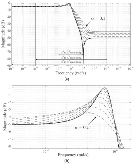
Figure 1. (a) Simulated magnitude responses of $(1+\alpha )$ lowpass fractional order transfer function for $\alpha =0.1$ to $0.9$ in steps of $0.1$ with coefficients selected to approximate elliptic response; and (b) details of passband ripple.

This transfer function will have a notch shaped magnitude response with low and high frequency gains of $a_4$ and $a_4{a}_1/a_2$, respectively, and an attenuation from passband to stopband dependent on $\alpha$. The magnitude expression for Equation (7) is given by

$$|H_{1+\alpha }\left(j\omega \right)|=a_4\frac{\sqrt{a_1^2{\omega }^{2+2\alpha }+2a_1{\omega }^{1+\alpha }cos\left(\frac{(1+\alpha )\pi }{2}\right)+1}}{\sqrt{a_2^2{\omega }^{2+2\alpha }+a_3^2{\omega }^{2\alpha }+2a_2{\omega }^{1+\alpha }cos\left(\frac{(1+\alpha )\pi }{2}\right)+2a_3{\omega }^{\alpha }cos\left(\frac{\alpha \pi }{2}\right)+1}}$$

(8)

where $\omega$ is the frequency in rad/s.

2.1. Coefficient Determination

In the design of traditional integer-order analog filters, the acceptable passband and stopband attenuations are used to calculate the necessary filter order based on the desired approximation (Butterworth, Chebyshev, Inverse Chebyshev, and elliptic) [21]. This calculated order is often a real-number that is rounded-up to the nearest integer value which is necessary to be realizable using integer-order filters. From this order, the necessary coefficients can be determined through provided design equations or from tables of available coefficients, which are further used in the implementation and realization of the necessary circuits. Additionally, optimization methods have also been explored to design these types of circuits [22,23].

Currently, fractional-order filter design does not yet have a comprehensive set of design procedures and tables of coefficients to support their realization. However, studies are ongoing to develop methods to design these filters [5,6,19], which also provides the motivation behind this study. Realizing an approximated elliptic response using Equation (7) that has both passband and stopband ripple characteristics requires the appropriate selection of the transfer function coefficients $[a_1,a_2,a_3,a_4]$. One method to determine these coefficients is through the application of optimization routines, and have been previously utilized for other filter designs [5,18,19]. In this work, a non-linear least squares optimization routine is applied to search for the coefficients of the fractional notch transfer function given by Equation (7) that yields the least error when compared to the second-order elliptic response given by Equation (6). This optimization problem is described by:

$$\underset{x}{min}\sum _{i=1}^k{\left(|H_{1+\alpha }\left(x,{\omega }_i\right)|-|E_2\left({\omega }_i\right)|\right)}^2$$

(9)

where x is the vector of filter coefficients, $|H_{1+\alpha }(x,{\omega }_i)|$ is the magnitude response using Equation (7) with x at frequency ${\omega }_i$ (rad/s), $|E_2\left({\omega }_i\right)|$ is the second order elliptic magnitude response given by Equation (6) at frequency ${\omega }_i$ (rad/s), and k is the total number of data points in the magnitude responses. The number of data points used in the fitting procedure $(k=9001)$ was selected to ensure that the ripple characteristics of the elliptic response were represented with sufficient frequency resolution within the dataset. The routine was implemented in MATLAB (v.2015b, 8.6.0.267246) using the fminsearch function with the default termination tolerances. The fminsearch function uses the simplex search method [24].

2.2. Symmetrical Fittings

It was noted previously in [20] that the frequency band used in the fitting procedure could impact the coefficients. However, this impact has not yet been formally investigated, providing the motivation for this exploration. This work quantifies the differences (in terms of coefficients and overall magnitude characteristics) that result from using different frequency bands in the optimization procedure. The least squares fitting procedure described by Equation (9) was applied to three symmetrical test cases. The three frequency bands were ${\omega }_{B1}ϵ\left[{10}^{-5},{10}^5\right]$ rad/s, ${\omega }_{B2}ϵ\left[{10}^{-3},{10}^3\right]$ rad/s, and ${\omega }_{B3}ϵ\left[{10}^{-1},{10}^1\right]$ rad/s. These frequency bands, labeled in Figure 1a, were selected because they each capture the passband ripple and transition to the stopband (which occurs between approximately ${10}^{-1}$ rad/s and ${10}^1$ rad/s). The wider ranges (${\omega }_{B1}$, ${\omega }_{B2}$) capture more data in the flat regions of the stopband and passband.

The coefficients determined for the fitting with each frequency band for $\alpha =0.1$ to $\alpha =0.9$ in $0.01$ steps are given in Figure 2. The solid lines in Figure 2 represent the coefficients using ${\omega }_{B1}$, dashed lines those using ${\omega }_{B2}$, and dash-dotted those using ${\omega }_{B3}$. The coefficients ($a_4$, $a_3$, $a_2$, $a_1$) are very similar for $\alpha >0.7$ for all fitting cases. The greatest differences between coefficients determined using the different frequency bands are observed at lower $\alpha$ values. Therefore, the difference in fitted frequency bands do not have a significant effect on the determined coefficients for $\alpha >0.7$ in these specific cases. Coefficients ($a_2$, $a_3$, $a_4$) all display a general trend of decreasing values for the cases using smaller frequency fitting bands (i.e., the fitting for ${\omega }_{B3}$ shows the lowest coefficient values for $a_2$, $a_3$, and $a_4$).

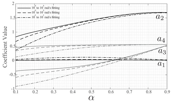
Figure 2. Coefficients of fractional-order transfer function in Equation (7) to approximate second-order elliptic characteristics applying least squares fitting to three symmetrical frequency ranges.

MATLAB simulations of Equation (8) using the ${\omega }_{B1}$ coefficients for $\alpha =0.1$ to $\alpha =0.9$ in steps of $0.1$ are given in Figure 1a as dashed lines. From these simulations, it is clear that this approximation method does realize the fractional-step attenuations (with the slope in the transition band strictly dependent on $\alpha$) but that there are further differences compared to the elliptic response. The most significant difference is that the HFG of each fractional-order case is higher than the $-50$ dB magnitude of the elliptic response (detailed in Figure 1a). Further, the passband ripple is smaller for each fractional-order case (detailed in Figure 1b) with the smallest passband ripple (i.e., the lowest passband gain) occurring for the $\alpha =0.1$ case. This case, given in Figure 1b, reaches approximately $-3.6$ dB compared to 0 dB of the second-order elliptic response. This is understandable, as $\alpha$ approaches zero the filter order is approaching 1, with first-order filters not able to provide any ripple or higher Q.

The differences in DC gain and HFG for each set of coefficients are further detailed in Figure 3 for $\alpha =0.1$ to $\alpha =0.9$ in steps of $0.01$. The solid, dashed, and dash-dotted lines correspond to those cases using the coefficients from the ${\omega }_{B1}$, ${\omega }_{B2}$, and ${\omega }_{B3}$ frequency bands, respectively. Observing the DC gains, the magnitude for each fitting is very close to the theoretical value of $-5$ dB for $\alpha >0.7$, but it decreases at lower values of $\alpha$. These deviations are most significant for the ${\omega }_{B3}$ fitting, which has a DC gain of approximately $-19$ dB for the $\alpha =0.1$ case. A similar trend is observed in the HFG, with the greatest deviations observed for the ${\omega }_{B3}$ fitting; though the most significant differences occur near $\alpha =0.5$ for the HFG. These low and high frequency gain differences highlight the impact that the selection of frequency range has on the determined coefficients using the optimization procedure. The ${\omega }_{B1}$ range contains the widest range of frequencies, which places a greater weighting on the optimization procedure to return coefficients that best fit these regions. This results in the DC gain and HFG that is closest to the elliptic case compared to coefficients determined using the ${\omega }_{B2}$ and ${\omega }_{B3}$ frequency bands.

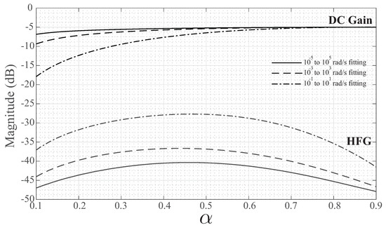
Figure 3. DC and high-frequency gain of fractional-order transfer function using coefficients to approximate elliptic characteristics.

2.3. Asymmetrical Fittings

In the previous fittings, each of the selected frequency bands were symmetrical in terms of the number of frequency decades included above and below 1 rad/s. However, it is possible to choose an asymmetrical frequency band to manipulate the distribution of data in the passband and stopband within the fitting routine. To evaluate the differences this causes in the returned coefficients, the fitting routine was applied to five different frequency bands: (i) ${\omega }_{B1}ϵ\left[{10}^{-5},{10}^5\right]$ rad/s; (ii) ${\omega }_{A2}ϵ\left[{10}^{-5},{10}^3\right]$ rad/s; (iii) ${\omega }_{A3}ϵ\left[{10}^{-5},{10}^1\right]$ rad/s; (iv) ${\omega }_{A4}ϵ\left[{10}^{-3},{10}^5\right]$ rad/s; and (v) ${\omega }_{A5}ϵ\left[{10}^{-1},{10}^5\right]$ rad/s. The frequency bands ${\omega }_{A2,A3}$ were selected to introduce a greater passband frequency range into the fitting procedure and ${\omega }_{A4,A5}$ were selected to introduce a greater stopband frequency range. These ranges are all within the frequency bands explored for the symmetrical fittings. Applying the previously described optimization fitting routine, the coefficients extracted from each frequency band for $\alpha =0.1$ to $\alpha =0.9$ in $0.01$ steps are given in Figure 4a,b. In Figure 4a, the solid lines represent the coefficients using ${\omega }_{B1}$, dashed lines those using ${\omega }_{A2}$, and dash-dotted those using ${\omega }_{A3}$. Note that in these cases the set of returned coefficients shows very few differences based on the different frequency bands. This suggests that the frequency range of the stopband has little effect on the coefficients when a large sampling of the passband is used. In Figure 4b, the solid lines represent the coefficients using ${\omega }_{B1}$, dashed lines those using ${\omega }_{A4}$, and dash-dotted those using ${\omega }_{A5}$. Similar to the symmetric results, the coefficients ($a_4$, $a_3$, $a_2$, $a_1$) are very similar for $\alpha >0.7$ for all fitting cases. That is, the greatest differences between the coefficients extracted using the different frequency bands are observed at lower $\alpha$ values, with a decreasing trend for coefficients ($a_2$, $a_3$, $a_4$) observed at lower $\alpha$ values.

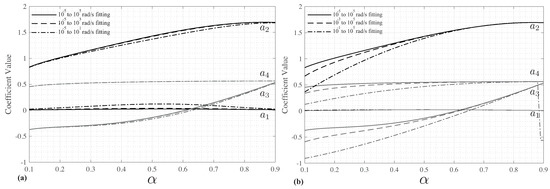
Figure 4. Coefficients of fractional-order transfer function in Equation (7) to approximate second-order elliptic characteristics applying least squares fitting to asymmetrical frequency ranges with: (a) lower limits of $\omega ={10}^{-5}$ rad/s; and (b) upper limits of $\omega ={10}^5$.

To further evaluate the differences of the asymmetric fitting frequency bands, the DC gain and HFG for $\alpha =0.1$ to $\alpha =0.9$ in steps of $0.01$ are detailed in Figure 5. Figure 5a presents the gains for ${\omega }_{B1}$ (solid), ${\omega }_{A2}$ (dashed), and ${\omega }_{A3}$ (dash-dotted). Observing the DC gains, the magnitude for each fitting is very close to the theoretical value of $-5$ dB for $\alpha >0.2$. This is not unexpected, since the DC gain is related to coefficient $a_4$, which is noted in Figure 4 to show very little variation for this set of asymmetrical fittings. Similar to the symmetric fittings, the HFG shows variation based on the frequency band, with the frequency band that includes the greatest number of data in the stopband (${\omega }_{A3}$) showing the closest agreement with the elliptic case. Figure 5b presents the gains for ${\omega }_{B1}$ (solid), ${\omega }_{A4}$ (dashed), and ${\omega }_{A5}$ (dash-dotted). In these cases, the HFG show similar values for all frequency fittings and the DC gains showing the greatest deviations. This confirms the previous expectations that the distribution of data in the passband and stopbands impacts the fitting process. With those frequency bands that have a larger representation of data yielding filter characteristics closer to the elliptic characteristics.

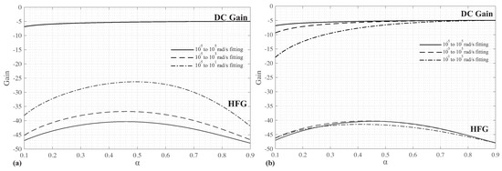
Figure 5. DC and high-frequency gain of fractional-order transfer function using coefficients from asymmetrical fittings using frequency ranges with: (a) lower limits of $\omega ={10}^{-5}$ rad/s; and (b) upper limits of $\omega ={10}^5$ to approximate elliptic characteristics.

2.4. Stability

Prior to designing hardware realizations of the fractional-order transfer functions, it is necessary to analyze them with the determined coefficients to ensure that they realize stable responses. Analyzing the stability of fractional-order systems is often accomplished by converting the s-domain transfer function to the W-plane defined in [25]. This transforms the transfer function from fractional order to integer order. This reduces the complexity of analyzing the stability by allowing traditional analysis methods to be employed. Applying this process to the denominator of Equation (7) yields the characteristic equation in the W-plane given by:

$$\begin{array}{ccc}\hfill a_2{W}^{m+k}+a_3{W}^k+1& =& 0\hfill \end{array}$$

(10)

From this characteristic equation, the roots of Equation (10) for $\alpha =0.1$ to $0.9$ were calculated with $k=10$ to 90, respectively, when $m=100$ using all sets of coefficients from both the symmetrical and asymmetrical fittings. The minimum root angles, $|{\theta }_W{|}_{\min }$, for each case of the symmetrical and asymmetrical fittings are given in Figure 6 and Figure 7. The minimum root angles are all greater than the minimum required angle for stability, $\left|{\theta }_W\right|>\frac{\pi }{2m}={0.9}^{\circ }$. This confirms that the fractional-order filters using the determined coefficients are stable for all fitted frequency ranges. It is interesting to note that the minimum phase angle for all fitted frequency ranges approaches a similar value (${1.07}^{\circ }$) as $\alpha$ approaches $0.9$ and the ${\omega }_{B1}$ case has the largest stability margin compared to the other cases.

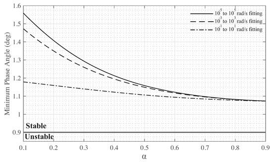
Figure 6. Minimum phase angle of roots of Equation (10) using coefficients from symmetrical frequency fittings.

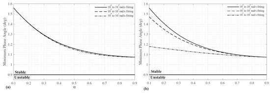
Figure 7. Minimum phase angle of roots of Equation (10) using coefficients from asymmetrical frequency fittings with: (a) lower limits of $\omega ={10}^{-5}$ rad/s; and (b) upper limits of $\omega ={10}^5$.

3. Fitted Frequency Range Comparison

To quantify the differences using coefficients from the different fitted frequency ranges, MATLAB simulations of the magnitude responses of Equation (7) for $\alpha =0.75$ and $\alpha =0.25$ are given in Figure 8. The solid, dashed, and dash-dotted lines represent the simulated responses using the coefficients from the optimization fittings applied to the ${\omega }_{B1}$, ${\omega }_{B2}$, and ${\omega }_{B3}$ frequency ranges, respectively. Each of these simulations used the coefficient values detailed in Figure 2. For the $\alpha =0.75$ case, the most significant differences are observed above 5 rad/s. Above this frequency, the stopband ripple occurs at the lowest frequency with the least attenuation when the coefficients from the smallest frequency band, ${\omega }_{B3}$ are used. These simulations support the results in Figure 3, with the ${\omega }_{B1}$ case yielding the closest high frequency gain to the elliptic case.

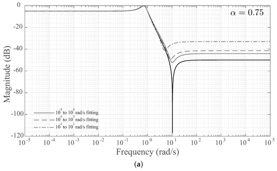
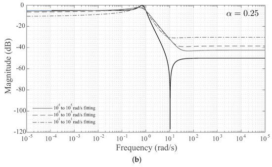
Figure 8. Simulated magnitude responses of (a) $(1+0.75)$ and (b) (1 + 0.25) lowpass fractional order transfer function using coefficients from different symmetrical frequency fitting ranges.

The magnitude characteristics of Equation (7) using the extracted coefficients from the asymmetrical fittings in Figure 4 for $\alpha =0.25$ and $\alpha =0.75$ are given in Figure 9 and Figure 10, respectively. These magnitude responses highlight the previous DC and HFG differences in Figure 5. For the coefficients derived using frequency bands with greater passband data (${\omega }_{A2,A3}$), the magnitude responses show very good agreement for both $\alpha =0.25$ and $\alpha =0.75$ up to 1 rad/s. At higher frequencies, the responses with fewer stopband data show poorer agreement with the elliptic response. This behavior is reversed in the magnitude responses that use the coefficients derived from the ${\omega }_{A4,A5}$. That is, the magnitude characteristics above 1 rad/s show very good agreement for all sets of coefficients for both $\alpha =0.25$ and $\alpha =0.75$ cases, resulting from the stopband containing the greatest number of data in the fittings, which results in the best fit of these region.

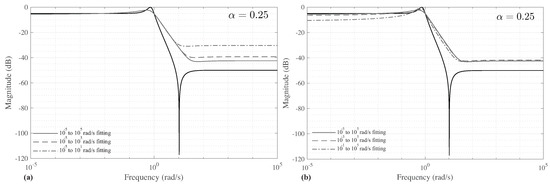
Figure 9. Simulated magnitude responses of $(1+0.25)$ lowpass fractional order transfer function using coefficients from different asymmetrical frequency fitting ranges with: (a) lower limits of $\omega ={10}^{-5}$ rad/s; and (b) upper limits of $\omega ={10}^5$.

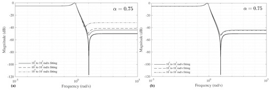
Figure 10. Simulated magnitude responses of $(1+0.75)$ lowpass fractional order transfer function using coefficients from different asymmetrical frequency fitting ranges with: (a) lower limits of $\omega ={10}^{-5}$ rad/s; and (b) upper limits of $\omega ={10}^5$.

Comparing the $\alpha =0.25$ cases of the symmetrical fittings in Figure 8, the coefficients have a significant impact on the HFG, DC gain and passband ripples of the magnitude characteristics. While the ${\omega }_{B3}$ case yields the most significant low- and high-frequency differences compared to the elliptic response, it has the closest approximation of the passband ripple. The elliptic response reaches a maximum of 0 dB, which is 5 dB above the DC gain, while the ${\omega }_{B3}$ case reaches $-0.40$ dB. For comparison, the ${\omega }_{B2}$ and ${\omega }_{B1}$ cases reach $-1.79$ dB and $-2.26$ dB, respectively. This is expected to be an impact of the frequency range, with the ${\omega }_{B2}$ and ${\omega }_{B1}$ fittings having a larger weighting (based on the distribution of data) to fit the high and low frequency bands which reduces the weighting of the interior band. As a result, the ${\omega }_{B3}$ case provides the coefficients that best approximate the magnitude characteristics in this band. This is also observed in the asymmetrical fittings of Figure 9, with the ${\omega }_{A4,A5}$ cases showing better agreement with the passband ripple than the ${\omega }_{A2,A3}$ cases. Again, this is a result of the ${\omega }_{A4,A5}$ cases having fewer data in the flat passband region to influence the fitting process.

It is clear the selection of frequency band for the optimization procedure does impact the coefficients. Therefore, the frequency band should be considered when employing optimization fitting processes to design a fractional-order filter. Designers must weigh the trade-offs that result between selecting a wider frequency band (necessary to capture the DC or high frequency gain) or a smaller specific band (necessary to capture the ripple characteristics); and decide based on which design features are most important for their specific application. Additionally, further studies should investigate the sensitivity of the fractional-order transfer functions magnitude characteristics to the coefficients, similar to that presented in [7]. This is important to understand during the physical implementation.

4. Circuit Simulations

To validate the proposed fractional-order filters with approximated elliptic characteristics, two cases were simulated and experimentally verified against the theoretical expectations. For these validations, two circuit topologies were selected and are given in Figure 11 where the component ${\mathrm{C}}_1$ is a fractional-order capacitor with impedance $Z_{C_1}=1/s^{\alpha }{C}_1$ and ${\mathrm{C}}_2$ is a traditional integer-order capacitor. The topologies in Figure 11a,b realize Equation (7) when the coefficient $a_3$ is positive and negative, respectively. It is necessary to present two topologies to realize the complete range of responses with the identified coefficients in this work, which take both positive and negative values depending on the value of $\alpha$.

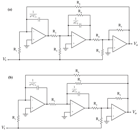
Figure 11. Circuit topologies to realize fractional-order low-pass notch filter response given by Equation (7) when $a_3$ is: (a) positive; and (b) negative. Note that in both topologies ${\mathrm{C}}_1$ is a fractional-order capacitor with impedance $Z_{C_1}=1/s^{\alpha }{C}_1$.

The topology in Figure 11a realizes the transfer function given by:

$$T_1^{1+\alpha }\left(s\right)=-\frac{R_6}{R_1}\frac{s^{1+\alpha }\frac{C_1{C}_2{R}_1{R}_2{R}_4}{R_3}+1}{s^{1+\alpha }\frac{C_1{C}_2{R}_2{R}_4{R}_6}{R_5}+s^{\alpha }\frac{C_1{R}_2{R}_6}{R_5}+1}=-a_4\frac{\frac{s^{1+\alpha }}{{\omega }_0^{1+\alpha }}{a}_1+1}{\frac{s^{1+\alpha }}{{\omega }_0^{1+\alpha }}{a}_2+\frac{s^{\alpha }}{{\omega }_0^{\alpha }}{a}_3+1}$$

(11)

and the topology in Figure 11b realizes the transfer function given by:

$$T_2^{1+\alpha }\left(s\right)=-\frac{R_6}{R_1}\frac{s^{1+\alpha }\frac{C_1{C}_2{R}_1{R}_2^2}{R_4}+1}{s^{1+\alpha }\frac{C_1{C}_2{R}_2^2{R}_6}{R_5}-s^{\alpha }\frac{C_1{R}_2{R}_6}{R_3}+1}=-a_4\frac{\frac{s^{1+\alpha }}{{\omega }_0^{1+\alpha }}{a}_1+1}{\frac{s^{1+\alpha }}{{\omega }_0^{1+\alpha }}{a}_2+\frac{s^{\alpha }}{{\omega }_0^{\alpha }}{a}_3+1}$$

(12)

Note that in both cases the term ${\omega }_0$ is the frequency scaling factor to shift the response from the normalized frequency of 1 rad/s.

The topology in Figure 11a with transfer function given by Equation (11) was used to realize a $(1+\alpha )=1.8$ order filter. For this case, the utilized coefficients were $a_1=0.01626$, $a_2=1.6844$, $a_3=0.3317$, and $a_4=0.5622$, selected from coefficients returned using the ${10}^{-5}$ rad/s to ${10}^5$ fitting bandwidth given in Figure 2. Using these coefficients, the necessary resistances and capacitances for the topology were calculated using the system of equations built by equating the coefficients in Equation (11) (i.e., $C_1{C}_2{R}_1{R}_2{R}_4/R_3=a_1/{\omega }_0^{1+\alpha }$; $C_1{C}_2{R}_2{R}_4{R}_6/R_5=a_2/{\omega }_0^{1+\alpha }$; $C_1{R}_2{R}_6/R_5=a_3/{\omega }_0^{\alpha }$; $R_6/R_1=a_4$). The specific resistors and capacitors are given in Table 1 when a frequency of ${\omega }_0=\left(2\pi \right)10$ krad/s is used. At this time, fractional-order capacitors are not available for either simulations or physical realizations and require the use of approximations; however, it is important to note the recent progress in realizing devices with fractional-order impedances [26,27,28]. For the simulations and experimental circuits in this work, the fractional-capacitors were approximated using the 5th order Foster-I topology given in Figure 12. The circuit components required to realize the $\alpha =0.8$ device were calculated using the process detailed in [29], with these calculated values given in Table 2. The experimental results were collected using an Omicron Bode 100 network analyzer from a circuit realized using discrete components on a breadboard. The approximated fractional-order capacitor was realized on a custom printed-circuit board (PCB) interfaced to the breadboard setup. This experimental test setup is shown in Figure 13a with the circuit implementation detailed in Figure 13b. The fractional-order capacitor PCB implementation is outlined in Figure 13b using the dashed box. The magnitude responses collected from both SPICE simulations and experimental implementations, using LT1361 operational amplifiers, are given in Figure 14a as dashed and dashed-dotted lines, respectively. For comparison to the simulation and experimental results, the theoretical magnitude response given by Equation (8) is a solid line in Figure 14a. Note that both simulations and experimental results show very good agreement with the theoretical response. The simulations show less than $0.21$ dB difference compared to the theoretical for frequencies below 70 kHz with a maximum deviation of $1.73$ dB occurring at 100 kHz.

Table 1. Component values to realize Equation (7) for the Figure 2 coefficients when $\alpha =0.8$ and $0.2$ using the topologies in Figure 11a,b, respectively.

$\mathit{\alpha }$	${\mathit{C}}_1$ (F s${}^{\mathit{\alpha }-1}$)	${\mathit{C}}_2$ (nF)	${\mathit{R}}_1$ ($\mathbf{\Omega }$)	${\mathit{R}}_2$ ($\mathbf{\Omega }$)	${\mathit{R}}_3$ ($\mathbf{\Omega }$)	${\mathit{R}}_4$ ($\mathbf{\Omega }$)	${\mathit{R}}_5$ ($\mathbf{\Omega }$)	${\mathit{R}}_6$ ($\mathbf{\Omega }$)
$0.8$	62n	10	1k	680	$90.8$k	$8.08$k	492	562
$0.2$	$46.9\mu$	$6.8$	$4.7$k	1k	$3.17$k	65k	428	$2.38$k

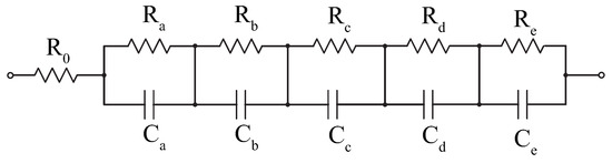
Figure 12. Foster-I circuit topology to realize a fifth order approximation of a fractional-order capacitor.

Table 2. Component values to realize fractional-order capacitors with $\alpha =0.8$ and $0.2$ using fifth order Foster I topology centered at 10 kHz.

$\mathit{\alpha }$	${\mathit{R}}_0$ ($\mathbf{\Omega }$)	${\mathit{R}}_{\mathit{a}}$ ($\mathbf{\Omega }$)	${\mathit{R}}_{\mathit{b}}$ ($\mathbf{\Omega }$)	${\mathit{R}}_{\mathit{c}}$ ($\mathbf{\Omega }$)	${\mathit{R}}_{\mathit{d}}$ ($\mathbf{\Omega }$)	${\mathit{R}}_{\mathit{e}}$ ($\mathbf{\Omega }$)	${\mathit{C}}_{\mathit{a}}$ (nF)	${\mathit{C}}_{\mathit{b}}$ (nF)	${\mathit{C}}_{\mathit{c}}$ (nF)	${\mathit{C}}_{\mathit{d}}$ (nF)	${\mathit{C}}_{\mathit{e}}$ (nF)
$0.8$	$58.8$	$65.1$	$326.4$	$1.47$k	$7.06$k	$84.23$k	$12.8$	$16.2$	$22.6$	$29.7$	$15.7$
$0.2$	$931.5$	$374.9$	$573.6$	$837.2$	$1.23$k	$1.93$k	$1.28$	$5.29$	$22.85$	$98.5$	$393.8$

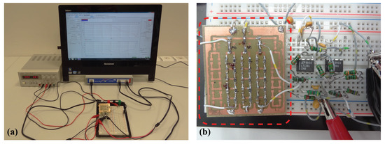
Figure 13. (a) Experimental setup to measure magnitude responses of approximated $(1+\alpha )$ order filters; and (b) breadboard implementation of topology using fifth order approximation of a fractional-order capacitor (outlined using the dashed box).

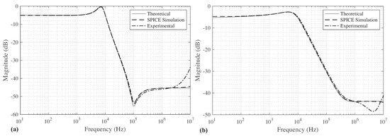
Figure 14. Theoretical (solid), SPICE simulated (dashed), and experimental (dashed-dotted) magnitude responses of (a) $(1+\alpha )=1.8$ and (b) $1.2$ order approximated elliptic filter responses.

Further, the topology in Figure 11b with transfer function given by Equation (12) was used to realize a $(1+\alpha )=1.2$ order filter. For this case, the utilized coefficients were $a_1=0.01320$, $a_2=1.1037$, $a_3=-0.3208$, and $a_4=0.5055$, selected from coefficients returned using the ${10}^{-5}$ rad/s to ${10}^5$ fitting bandwidth given in Figure 2. Using these coefficients, the necessary resistances and capacitances for the topology were calculated using the system of equations built by equating coefficients in Equation (12) (i.e., $C_1{C}_2{R}_1{R}_2^2/R_4=a_1/{\omega }_0^{1+\alpha }$; $C_1{C}_2{R}_2^2{R}_6/R_5=a_2/{\omega }_0^{1+\alpha }$; $-C_1{R}_2{R}_6/R_3=a_3/{\omega }_0^{\alpha }$; $R_6/R_1=a_4$). The specific resistors and capacitors are given in Table 1 when a frequency of ${\omega }_0=\left(2\pi \right)10$ krad/s is used and the $C_1$, $C_2$, $R_1$, $R_2$ values are initially chosen, and the other values are computed. The circuit components required to realize the $\alpha =0.2$ device are also given in Table 2. The magnitude responses collected from both SPICE simulations and experimental implementations are given in Figure 14b as dashed and dashed-dotted lines, respectively, compared to the theoretical response given as a solid line. Again, both simulation and experimental results show very good agreement with the theoretical response. The simulations show less than $0.1$ dB difference compared to the theoretical for $100\mathrm{Hz}<f<100\mathrm{kHz}$ with a maximum deviation of $0.49$ dB occurring at 10 Hz. From the experimental results of both filters in Figure 14, the deviation at frequencies above 1 MHz are likely a result of parasitics in the breadboard implementation of these circuits.

To validate the stability of each constructed filter circuit, the transient responses were collected for both $(1+\alpha )=1.2$ and $1.8$ order filters when applying a 800 Hz square wave input signal. Both the input (solid) and output (dashed) waveforms during this transient test are given in Figure 15a,b for the $1.2$ and $1.8$ order filters, respectively. In both cases, the output waveforms confirm that the circuits are stable and validate the previous stability analyses. The oscillations in the transient response of the $1.8$ order filter in Figure 15b confirm the results in the stability analysis, that is, that the filters with higher $\alpha$ have less stability margin. Both simulation and experimental results serve to validate the proposed $(1+\alpha )$ fractional-order elliptic filter responses and that both topologies are appropriate in realizing these designs.

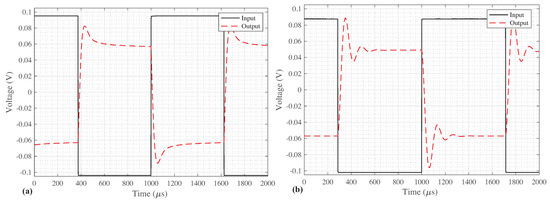
Figure 15. Transient responses (dashed) of experimentally realized (a) $(1+\alpha )=1.2$ and (b) $1.8$ order approximated elliptic filter responses when applying a 800 Hz square wave input (solid).

5. Summary of Optimization Procedure

While the coefficients presented in Figure 2 and Figure 4 can be used to implement the approximated fractional-order elliptic responses in this work, to realize responses with different ripple characteristics requires calculation of different sets of coefficients. To support the adoption of the process used in this work to calculate further sets of coefficients for different characteristics, the steps are summarized below:

• Select desired second-order elliptic magnitude characteristics to approximate with fractional-order filter:

  (a)

  Passband ripple (5 dB in this work).

  (b)

  Stopband attenuation ($-50$ dB in this work).

• Select target frequency band to use for procedure fitting.
• Implement objective function given by Equation (9) using desired elliptic response and fractional-order transfer function given by Equation (7).
• Apply optimization solver to objective function to evaluate coefficients for target filter order (1 + $\alpha$).
• Evaluate stability of fractional-order filter with solved coefficients using W-plane transformations.
• Select appropriate circuit topology to realize fractional-order transfer function.
• Calculate necessary component values to realize target coefficients for desired center frequency.

6. Conclusions

An optimization fitting procedure was applied in this work to design low-pass fractional-order filters with passband and stopband ripples to approximate the traditional elliptic characteristics. The fractional-order filter coefficients were determined using symmetrical and asymmetrical frequency bands, with all coefficients yielding stable responses. While this method does realize fractional-step attenuations in the transition from passband to stopband, it also shows limits in the presented cases to approximate the low- and high-frequency behavior. Of significant note is that the choice of frequency range used with the optimization procedure significantly impacts the coefficients and magnitude response of the approximated transfer function. For the cases explored in this work, the wider frequency ranges yielded better DC gains and HFG, but at the cost of poorer approximations of the ripple characteristics. The simulated and experimental magnitude responses from filter circuits with order $(1+\alpha )=1.2$ and $1.8$ realized using approximated fractional-order capacitors validate the proposed circuits and their fractional-order characteristics, and confirm their stability. The simulation and experimental validation of the filter structure to realize negative $a_3$ coefficients in this work expands the range of available topologies for designers exploring fractional-order filter implementations.

References

- Oldham, K.B.; Spanier, J. The Fractional Calculus: Theory and Applications of Differentiation and Integration to Arbitrary Order; Academic Press: New York, NY, USA, 1974. [Google Scholar]
- Podlubny, I. Fractional Differential Equations; Academic Press: London, UK, 1999. [Google Scholar]
- Ortigueira, M.D. Fractional Calculus for Scientists and Engineers; Springer: Heidelberg, Germany, 2011. [Google Scholar]
- Soltan, A.; Radwan, A.G.; Soliman, A.M. Fractional order Sallen-Key and KHN filters: Stability and poles allocation. Circ. Syst. Signal Process. 2015, 34, 1461–1480. [Google Scholar] [CrossRef]
- Freeborn, T.J.; Elwakil, A.S.; Maundy, B. Approximated fractional-order Inverse Chebyshev lowpass filters. Circ. Syst. Signal Process. 2016, 35, 1973–1982. [Google Scholar] [CrossRef]
- Kubanek, D.; Freeborn, T.J. (1 + α) Fractional-order transfer functions to approximate low-pass magnitude responses with arbitrary quality factor. AEU Int. J. Electron. Commun. 2018, 83, 570–578. [Google Scholar] [CrossRef]
- Kubanek, D.; Freeborn, T.J.; Koton, J.; Herencsar, N. Evaluation of (1 + α) fractional-order approximated Butterworth high-pass and band-pass filter transfer functions. Elektronika ir Elektrotechnika 2018, 24, 37–41. [Google Scholar] [CrossRef]
- Baranowski, J.; Pauluk, M.; Tutaj, A. Analog realization of fractional filters: Laguerre approximation approach. AEU-Int. J. Electron. Commun. 2018, 81, 1–11. [Google Scholar] [CrossRef]
- Ahmadi, P.; Maundy, B.; Elwakil, A.S.; Belostotski, L. High-quality factor asymmetric-slope band-pass filters: A fractional-order capacitor approach. IET Circ. Devices Syst. 2012, 6, 187–198. [Google Scholar] [CrossRef]
- Bertsias, P.; Khateb, F.; Kubanek, D.; Khanday, F.A.; Psychalinos, C. Capacitorless Digitally Programmable Fractional-Order Filters. AEU Int. J. Electron. Commun. 2017, 78, 228–237. [Google Scholar] [CrossRef]
- Jerabek, J.; Sotner, R.; Dvorak, J.; Polak, J.; Kubanek, D.; Herencsar, N.; Koton, J. Reconfigurable fractional-order filter with electronically controllable slope of attenuation, pole frequency and type of approximation. J. Circ. Syst. Comput. 2017, 26, 1750157. [Google Scholar] [CrossRef]
- AbdelAty, A.M.; Soltan, A.; Ahmed, W.A.; Radwan, A.G. On the analysis and design of fractional-order Chebyshev complex filter. Circ. Syst. Signal Process. 2018, 37, 915–938. [Google Scholar] [CrossRef]
- Hamed, E.M.; AbdelAty, A.M.; Said, L.A.; Radwan, A.G. Effect of different approximation techniques on fractional-order KHN filter design. Circ. Syst. Signal Process. 2018, 1–31. [Google Scholar] [CrossRef]
- Tsirimokou, G.; Laoudias, C.; Psychalinos, C. 0.5-V fractional-order companding filters. Int. J. Circ. Theory Appl. 2015, 43, 1105–1126. [Google Scholar] [CrossRef]
- Baranowski, B.; Piatek, P. Fractional band-pass filters: Design, implementation and application to EEG signal processing. J. Circ. Syst. Comput. 2017, 26, 1750170. [Google Scholar] [CrossRef]
- Tolba, M.F.; AbdelAty, A.M.; Soliman, N.S.; Said, L.A.; Madian, A.H.; Azar, A.T.; Radwan, A.G. FPGA implementation of two fractional order chaotic systems. AEU Int. J. Electron. Commun. 2017, 78, 162–172. [Google Scholar] [CrossRef]
- Tolba, M.F.; AboAlNaga, B.M.; Said, L.A.; Madian, A.H.; Radwan, A.G. Fractional order integrator/ differentiator: FPGA implementation and FOPID controller application. AEU Int. J. Electron. Commun. 2019, 98, 220–229. [Google Scholar] [CrossRef]
- Mahata, S.; Saha, S.K.; Kar, R.; Mandal, D. Optimal design of fractional-order low pass Butterworth filter with accurate magnitude response. Digit. Signal Process. 2018, 72, 96–114. [Google Scholar] [CrossRef]
- Freeborn, T.J.; Maundy, B.; Elwakil, A.S. Approximated fractional order Chebyshev lowpass filters. Math. Probl. Eng. 2014. [Google Scholar] [CrossRef]
- Freeborn, T.J.; Kubanek, D.; Koton, J.; Dvorak, J. Fractional-order lowpass elliptic responses of (1 + α)-order transfer functions. In Proceedings of the 2018 IEEE International Conference on Digital Signal Processing, Athens, Greece, 4–6 July 2018; pp. 346–349. [Google Scholar] [CrossRef]
- Schaumann, R.; Xiao, H.; Van Valkenburg, M.E. Design of Analog Filters; Oxford University Press: Oxford, UK, 2010. [Google Scholar]
- Le, T.H.; Van Barel, M. A convex optimization method to solve a filter design problem. J. Comput. Appl. Math. 2014, 255, 183–192. [Google Scholar] [CrossRef]
- Le, T.H.; Van Barel, M. A convex optimization model for finding non-negative polynomials. J. Comput. Appl. Math. 2016, 301, 121–134. [Google Scholar] [CrossRef]
- Lagarias, J.C.; Reeds, J.A.; Wright, M.H.; Wright, P.E. Convergence properties of the Nelder-Mead simplex method in low dimensions. SIAM J. Optim. 1998, 9, 112–147. [Google Scholar] [CrossRef]
- Radwan, A.; Soliman, A.; Elwakil, A.; Sedeek, A. On the stability of linear systems with fractional-order elements. Chaos Solit. Fract. 2009, 40, 2317–2328. [Google Scholar] [CrossRef]
- Agambayev, A.; Patole, S.; Bagci, H.; Salama, K.N. Tunable fractional-order capacitor using layered ferroelectric polymers. AIP Adv. 2017, 7, 095202. [Google Scholar] [CrossRef]
- Agambayev, A.; Rajab, K.H.; Hassan, A.H.; Farhat, M.; Bagci, H.; Salama, K.N. Towards fractional-order capacitors with broad tunable constant phase angles: Multi-walled carbon nanotube-polymer composite as a case study. J. Phys. D Appl. Phys. 2018, 51, 065602. [Google Scholar] [CrossRef]
- Agambayev, A.; Farhat, M.; Patole, S.P.; Hassan, A.H.; Bagci, H.; Salama, K.N. An ultra-broadband single-component fractional-order capacitor using MoS2-ferroelectric polymer composite. Appl. Phys. Lett. 2018, 113, 093505. [Google Scholar] [CrossRef]
- Tsirimokou, G. A systematic procedure for deriving RC networks of fractional-order elements emulators using MATLAB. AEU Int. J. Electron. Commun. 2017, 78, 7–14. [Google Scholar] [CrossRef]
© 2018 by the authors. Licensee MDPI, Basel, Switzerland. This article is an open access article distributed under the terms and conditions of the Creative Commons Attribution (CC BY) license (http://creativecommons.org/licenses/by/4.0/).