Prediction of Douglas-Fir Lumber Properties: Comparison between a Benchtop Near-Infrared Spectrometer and Hyperspectral Imaging System


Abstract
:Featured Application
Abstract
1. Introduction
2. Materials and Methods
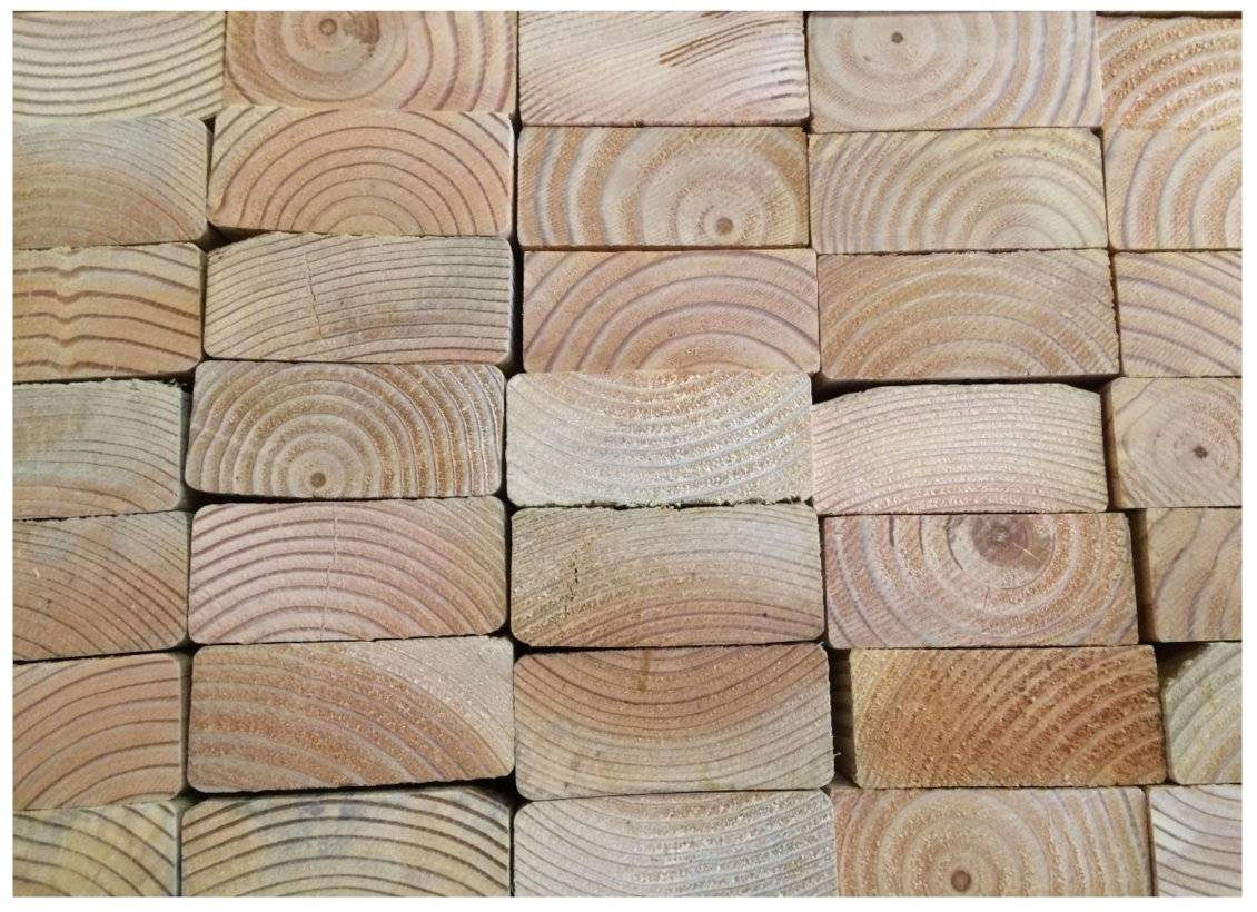
2.1. Specimen Preparation and Testing
2.2. Near-Infrared Spectroscopy
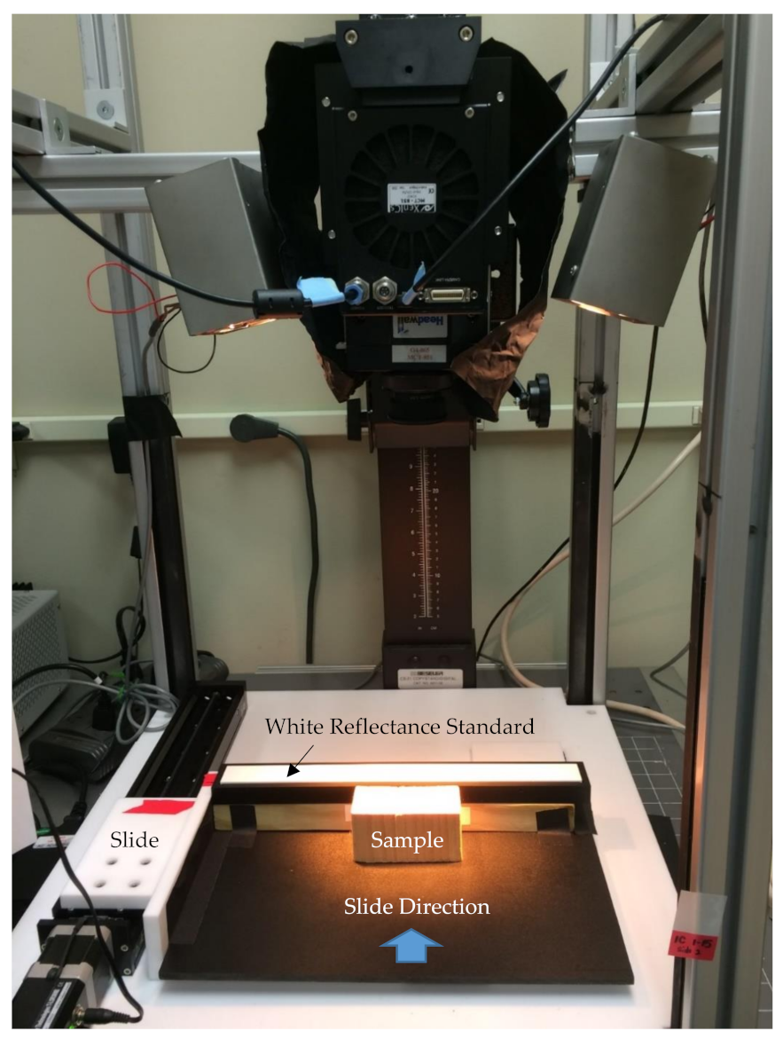
2.3. Hyperspectral Imaging
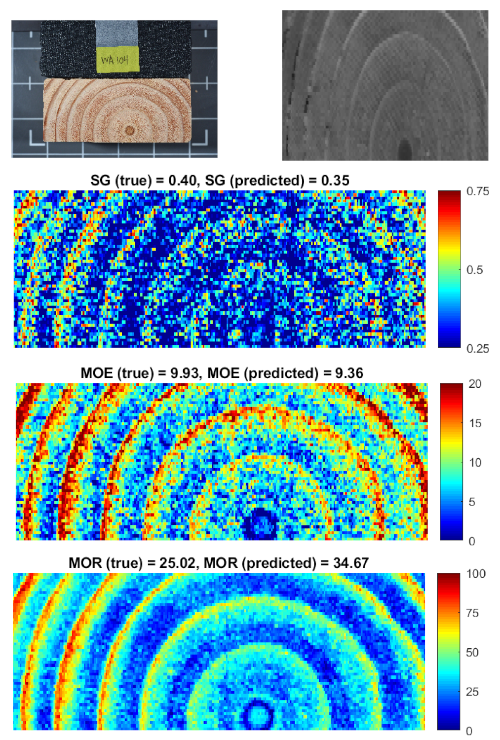
2.4. Hyperspectral Imaging Data Processing
2.5. Wood Property Calibration and Prediction of Wood Properties
3. Results
4. Discussion
5. Conclusions
Supplementary Materials
Author Contributions
Acknowledgments
Conflicts of Interest
References
- Howard, J. US Timber Production, Trade, Consumption, and Price Statistics 1965 to 2005; Research Paper FPL-RP-637; U.S. Department of Agriculture, Forest Service, Forest Products Laboratory: Madison, WI, USA, 2007; p. 91.
- Huang, C.L.; Briggs, D.G.; Lowell, E. Log lumber value of type II thinned Douglas-fir installations. In Stand Management Cooperative quarterly news, 3rd Quarter; School of Forest Resources, University of Washington: Seattle, WA, USA, 2011. [Google Scholar]
- Azuma, D.L.; Bednar, L.F.; Heserote, B.A.; Veneklase, C.F. Timber Resource Statistics for Western Oregon, 1997; Resource Bulletin PNW-RB-237; U.S. Department of Agriculture, Forest Service, Pacific Northwest Research Station: Portland, OR, USA, 2004; p. 120.
- Adams, W.T.; Hobbs, S.; Johnson, N. Intensively managed forest plantations in the Pacific Northwest, Conclusions. J. For. 2005, 103, 99–100. [Google Scholar]
- Gray, A.N.; Veneklase, C.F.; Rhoads, R.D. Timber Resource Statistics for Nonnational Forest Land in Western Washington, 2001; Resource Bulletin PNW-RB-246; U.S. Department of Agriculture, Forest Service, Pacific Northwest Research Station: Portland, OR, USA, 2005; p. 117.
- Talbert, C.; Marshall, D. Plantation productivity in the Douglas-fir region under intensive silvicultural practices: Results from research and operations. J. For. 2005, 103, 65–70. [Google Scholar]
- Gartner, B.L. Assessing wood characteristics and wood quality in intensively managed plantations. J. For. 2005, 103, 75. [Google Scholar]
- Vikram, V.; Cherry, M.L.; Briggs, D.; Cress, D.W.; Evans, R.; Howe, G.T. Stiffness of Douglas-fir lumber: Effects of wood properties and genetics. Can. J. For. Res. 2011, 41, 1160–1173. [Google Scholar] [CrossRef]
- Moore, J.R.; Cown, D.J. Corewood (juvenile wood) and its impact on wood utilisation. Curr. For. Rep. 2017, 3, 107–118. [Google Scholar] [CrossRef]
- Ross, R.J.; McDonald, K.A.; Green, D.W.; Schad, K.C. Relationship between log and lumber modulus of elasticity. For. Prod. J. 1997, 47, 89–92. [Google Scholar]
- Wang, X.; Ross, R.J.; Mattson, J.A.; Erickson, J.R.; Forsman, J.W.; Geske, E.A.; Wehr, M.A. Nondestructive evaluation techniques for assessing modulus of elasticity and stiffness of small-diameter logs. For. Prod. J. 2002, 52, 79–86. [Google Scholar]
- Carter, P.; Chauhan, S.; Walker, J. Sorting logs and lumber for stiffness using Director HM200. Wood Fiber Sci. 2006, 38, 49–54. [Google Scholar]
- Wang, X. Acoustic measurements on trees and logs: A review and analysis. Wood Sci. Technol. 2013, 47, 965–975. [Google Scholar] [CrossRef]
- Wang, X.; Verrill, S.; Lowell, E.; Ross, R.J.; Herian, V.L. Acoustic sorting models for improved log segregation. Wood Fiber Sci. 2013, 45, 343–352. [Google Scholar]
- Moore, J.R.; Lyon, A.J.; Searles, G.J.; Lehneke, S.A.; Ridley-Ellis, D.J. Within- and between-stand variation in selected properties of Sitka spruce sawn timber in the UK: Implications for segregation and grade recovery. Ann. For. Sci. 2003, 70, 403–415. [Google Scholar] [CrossRef]
- Butler, A.; Dahlen, J.; Eberhardt, T.L.; Montes, C.; Antony, F.; Daniels, R.F. Acoustic evaluation of loblolly pine tree- and lumber-length logs allows for segregation of lumber modulus of elasticity, not for modulus of rupture. Ann. For. Sci. 2017, 74, 20. [Google Scholar] [CrossRef]
- Dahlen, J.; Montes, C.; Eberhardt, T.L.; Auty, D. Probability models that relate nondestructive test methods to lumber design values of plantation loblolly pine. Forestry 2018, 91, 295–306. [Google Scholar] [CrossRef]
- Zhou, Z.-R.; Zhao, M.-C.; Wang, Z.; Wang, B.J.; Guan, X. Acoustic testing and sorting of Chinese poplar logs for structural LVL products. BioResources 2013, 8, 4101–4116. [Google Scholar] [CrossRef]
- Achim, A.; Paradis, N.; Carter, P.; Hernández, R.E. Using acoustic sensors to improve the efficiency of the forest value chain in Canada: A case study with laminated veneer lumber. Sensors 2011, 11, 5716–5728. [Google Scholar] [CrossRef] [PubMed]
- Gindl, W.; Teischinger, A.; Schwanninger, M.; Hinterstoisser, B. The relationship between near infrared spectra of radial wood surfaces and wood mechanical properties. J. Near Infrared Spectrosc. 2001, 9, 255–261. [Google Scholar] [CrossRef]
- Kelley, S.S.; Rials, T.G.; Groom, L.H.; So, C.L. Use of infrared spectroscopy to predict the mechanical properties of six softwoods. Holzforschung 2004, 58, 252–260. [Google Scholar] [CrossRef]
- Schimleck, L.R.; Jones, P.D.; Clark, A.; Daniels, R.F.; Peter, G.F. Near infrared spectroscopy for the nondestructive estimation of clear wood properties of Pinus taeda L. from the southern United States. For. Prod. J. 2005, 55, 21–28. [Google Scholar]
- Haartveit, E.Y.; Flæte, P.O. Rapid prediction of basic wood properties by near infrared spectroscopy. N. Z. J. For. Sci. 2006, 36, 393. [Google Scholar]
- Hein, P.R.G.; Brancheriau, L.; Trugilho, P.F.; Lima, J.T.; Chaix, G. Resonance and near infrared spectroscopy for evaluating dynamic wood properties. J. Near Infrared Spectrosc. 2010, 18, 443–454. [Google Scholar] [CrossRef]
- Dahlen, J.; Diaz, I.; Schimleck, L.R.; Jones, P.D. Near-infrared spectroscopy prediction of southern pine No. 2 lumber physical and mechanical properties. Wood Sci. Technol. 2017, 51, 309–322. [Google Scholar] [CrossRef]
- Hoffmeyer, P.; Pedersen, J.G. Evaluation of density and strength of Norway spruce by near infrared reflectance spectroscopy. Holz Roh Werkst. 1995, 53, 165–170. [Google Scholar] [CrossRef]
- Meder, R.; Thumm, A.; Marston, D. Sawmill trial of at-line prediction of recovered lumber stiffness by NIR spectroscopy of Pinus radiata cants. J. Near Infrared Spectrosc. 2003, 11, 137–143. [Google Scholar] [CrossRef]
- Fujimoto, T.; Kurata, Y.; Matsumoto, K.; Tsuchikawa, S. Application of near infrared spectroscopy for estimating wood mechanical properties of small clear and full length lumber specimens. J. Near Infrared Spectrosc. 2008, 16, 529–537. [Google Scholar] [CrossRef]
- Fujimoto, T.; Kurata, Y.; Matsumoto, K.; Tsuchikawa, S. Feasibility of near-infrared spectroscopy for on-line grading of sawn lumber. Appl. Spectrosc. 2010, 64, 92–99. [Google Scholar] [CrossRef] [PubMed]
- Kobori, H.; Inagaki, T.; Fujimoto, T.; Okura, T.; Tsuchikawa, S. Fast online NIR technique to predict MOE and moisture content of sawn lumber. Holzforschung 2015, 69, 329–335. [Google Scholar] [CrossRef]
- Lu, G.; Fei, B. Medical hyperspectral imaging: A review. J. Biomed. Opt. 2014, 19, 010901. [Google Scholar] [CrossRef] [PubMed]
- Elmasry, G.; Kamruzzaman, M.; Sun, D.W.; Allen, P. Principles and applications of hyperspectral imaging in quality evaluation of agro-food products: A review. Crit. Rev. Food Sci. Nutr. 2012, 52, 999–1023. [Google Scholar] [CrossRef]
- Liu, Y.W.; Pu, H.B.; Sun, D.W. Hyperspectral imaging technique for evaluating food quality and safety during various processes: A review of recent applications. Trends Food Sci. Technol. 2017, 69, 25–35. [Google Scholar] [CrossRef]
- Manley, M. Near-infrared spectroscopy and hyperspectral imaging: Non-destructive analysis of biological materials. Chem. Soc. Rev. 2014, 43, 8200–8214. [Google Scholar] [CrossRef]
- Mishra, P.; Asaari, M.S.M.; Herrero-Langreo, A.; Lohumi, S.; Diezma, B.; Scheunders, P. Close range hyperspectral imaging of plants: A review. Biosyst. Eng. 2017, 164, 49–67. [Google Scholar] [CrossRef]
- Burger, J.; Gowen, A. Data handling in hyperspectral image analysis. Chemom. Intell. Lab. Syst. 2011, 108, 13–22. [Google Scholar] [CrossRef]
- Hagman, O. Multivariate prediction of wood surface features using an imaging spectrograph. Holz Roh Werkst. 1997, 55, 377–382. [Google Scholar] [CrossRef]
- Nystrom, J.; Hagman, O. Real-time spectral classification of compression wood in Picea abies. J. Wood Sci. 1999, 45, 30–37. [Google Scholar] [CrossRef]
- Duncker, P.; Spiecker, H. Detection and classification of Norway spruce compression wood in reflected light by means of hyperspectral image analysis. IAWA J. 2009, 30, 59–70. [Google Scholar] [CrossRef]
- Jones, P.D.; Schimleck, L.R.; So, C.L.; Clark, A.; Daniels, R.F. High resolution scanning of radial strips cut from increment cores by near infrared spectroscopy. IAWA J. 2007, 28, 473–484. [Google Scholar] [CrossRef]
- Fernandes, A.; Lousada, J.; Morais, J.; Xavier, J.; Pereira, J.; Melo-Pinto, P. Comparison between neural networks and partial least squares for intra-growth ring wood density measurement with hyperspectral imaging. Comput. Electron. Agric. 2013, 94, 71–81. [Google Scholar] [CrossRef]
- Fernandes, A.; Lousada, J.; Morais, J.; Xavier, J.; Pereira, J.; Melo-Pinto, P. Measurement of intra-ring wood density by means of imaging VIS/NIR spectroscopy (hyperspectral imaging). Holzforschung 2013, 67, 59–65. [Google Scholar] [CrossRef]
- Ma, T.; Inagaki, T.; Tsuchikawa, S. Calibration of SilviScan data of Cryptomeria japonica wood concerning density and microfibril angles with NIR hyperspectral imaging with high spatial resolution. Holzforschung 2017, 71, 341–347. [Google Scholar] [CrossRef]
- Thumm, A.; Riddell, M.; Nanayakkara, B.; Harrington, J.; Meder, R. Near infrared hyperspectral imaging applied to mapping chemical composition in wood samples. J. Near Infrared Spectrosc. 2010, 18, 507–515. [Google Scholar] [CrossRef]
- Thumm, A.; Riddell, M.; Nanayakkara, B.; Harrington, J.; Meder, R. Mapping within-stem variation of chemical composition by near infrared hyperspectral imaging. J. Near Infrared Spectrosc. 2016, 24, 605–616. [Google Scholar] [CrossRef]
- Meder, R.; Meglen, R.R. Near infrared spectroscopic and hyperspectral imaging of compression wood in Pinus radiata D. Don. J. Near Infrared Spectrosc. 2012, 20, 583–589. [Google Scholar] [CrossRef]
- Thumm, A.; Riddell, M. Resin defect detection in appearance lumber using 2D NIR spectroscopy. Eur. J. Wood Wood Prod. 2017, 75, 995–1002. [Google Scholar] [CrossRef]
- Mora, C.; Schimleck, L.R.; Yoon, S.C.; Thai, C.N. Determination of basic density and moisture content of loblolly pine wood disks using a near-infrared hyperspectral imaging system. J. Near Infrared Spectrosc. 2011, 19, 401–409. [Google Scholar] [CrossRef]
- Haddadi, A.; Burger, J.; Leblon, B.; Pirouz, Z.; Groves, K.; Nader, J. Using near-infrared hyperspectral images on subalpine fire board. Part 1: Moisture content estimation. Wood Mater. Sci. Eng. 2015, 10, 27–40. [Google Scholar] [CrossRef]
- Haddadi, A.; Burger, J.; Leblon, B.; Pirouz, Z.; Groves, K.; Nader, J. Using near-infrared hyperspectral images on subalpine fire board. Part 2: Density and basic specific gravity estimation. Wood Mater. Sci. Eng. 2015, 10, 41–56. [Google Scholar] [CrossRef]
- Lestander, T.A.; Geladi, P.; Larsson, S.H.; Thyrel, M. Near infrared image analysis for online identification and separation of wood chips with elevated levels of extractives. J. Near Infrared Spectrosc. 2012, 20, 591–599. [Google Scholar] [CrossRef]
- Dahlen, J.; Jones, P.D.; Seale, R.D.; Shmulsky, R. Mill variation in bending strength and stiffness of in-grade Douglas-fir No. 2 2 × 4 lumber. Wood Sci. Technol. 2013, 47, 1167–1176. [Google Scholar] [CrossRef]
- ASTM International. ASTM D4761-13: Standard Test Methods for Mechanical Properties of Lumber and Wood-Base Structural Material; ASTM International: West Conshohocken, PA, USA, 2013. [Google Scholar]
- ASTM International. ASTM D198-15: Standard Test Methods of Static Tests of Lumber in Structural Sizes; ASTM International: West Conshohocken, PA, USA, 2015. [Google Scholar]
- ASTM International. ASTM D1990-16: Standard Practice for Establishing Allowable Properties for Visually-Graded Dimension Lumber from in-Grade Tests of Full-Size Specimens; ASTM International: West Conshohocken, PA, USA, 2016. [Google Scholar]
- R Core Team. R: A Language and Environment for Statistical Computing; R Foundation for Statistical Computing: Vienna, Austria, 2018; Available online: http://www.R-project.org/ (accessed on 18 April 2018).
- RStudio. RStudio: Integrated Development Environment for R; RStudio: Boston, MA, USA, 2018; Available online: https://www.rstudio.com/ (accessed on 18 April 2018).
- Auguie, B. gridExtra: Miscellaneous Functions for “grid” Graphics. R Package Version 2.2.1. 2016. Available online: https://CRAN.R-project.org/package=gridExtra (accessed on 18 April 2018).
- Mevik, B.-H.; Wehrens, R.; Liland, K.H. pls: Partial Least Squares and Principal Component Regression. R Package Version 2.4-3. 2013. Available online: http://CRAN.R-project.org/package=pls (accessed on 18 April 2018).
- Stevens, A.; Ramirez-Lopez, L. An Introduction to the Prospectr Package. R Package Vignette R Package Version 0.1.3. 2013. Available online: https://cran.r-project.org/web/packages/prospectr/vignettes/prospectr-intro.pdf (accessed on 18 April 2018).
- Signal Developers Signal: Signal Processing. 2013. Available online: http://r-forge.r-project.org/projects/signal/ (accessed on 18 April 2018).
- Wickham and Rstudio Tidyverse: Easily Install and Load the ‘Tidyverse’ R Package Version 1.2.1. 2017. Available online: https://cran.r-project.org/web/packages/tidyverse/index.html (accessed on 18 April 2018).
- Savitzky, A.; Golay, M.J.E. Smoothing and differentiation of data by simplified least squares procedures. Anal. Chem. 1964, 36, 1627–1639. [Google Scholar] [CrossRef]
- Snee, R.D. Validation of regression models: Methods and examples. Technometrics 1977, 19, 415–428. [Google Scholar] [CrossRef]
- Mora, C.; Schimleck, L.R. On the selection of samples for multivariate regression analysis: Application to near infrared (NIR) calibration models. Can. J. For. Res. 2008, 38, 2626–2634. [Google Scholar] [CrossRef]
- Williams, P.C.; Sobering, D.C. Comparison of commercial near infrared transmittance and reflectance instruments for the analysis of whole grains and seeds. J. Near Infrared Spectrosc. 1993, 1, 25–32. [Google Scholar] [CrossRef]
- Kimberley, M.O.; McKinley, R.B.; Cown, D.J.; Moore, J.R. Modelling the variation in wood density of New Zealand-grown Douglas-fir. N. Z. J. For. Sci. 2017, 47, 15. [Google Scholar] [CrossRef]
- AACC 39-00.01, Near-Infrared Methods—Guidelines for Model Development and Maintenance; AAAC International: St. Paul, MN, USA, 1999.
- Schimleck, L.R.; Matos, J.L.M.; Trianoski, R.; Prata, J.G. Comparison of methods for estimating mechanical properties of wood by NIR spectroscopy. J. Spectrosc. 2018, 4823285. [Google Scholar] [CrossRef]
- Jordan, L.; He, R.; Hall, D.B.; Clark, A.; Daniels, R.F. Variation in loblolly pine ring microfibril angle in the Southeastern United States. Wood Fiber Sci. 2007, 39, 352–363. [Google Scholar]
- Jordan, L.; Clark, A.; Schimleck, L.R.; Hall, D.; Daniels, R.F. Regional variation in wood specific gravity of planted loblolly pine in the United States. Can. J. For. Res. 2008, 38, 698–710. [Google Scholar] [CrossRef]
- Filipescu, C.N.; Stoehr, M.U.; Pigott, D.R. Variation of lumber properties in genetically improved full-sib families of Douglas-fir in British Columbia, Canada. Forestry 2018, 3, 320–326. [Google Scholar] [CrossRef]
- Roblot, G.; Bléron, L.; Mériaudeau, F.; Marchal, R. Automatic computation of the knot area ratio for machine strength grading of Douglas-fir and Spruce timber. Eur. J. Environ. Civ. Eng. 2010, 14, 1317–1332. [Google Scholar] [CrossRef]
- Butler, M.A.; Dahlen, J.; Antony, F.; Kane, M.; Eberhardt, T.L.; Jin, H.; Love-Myers, K.; McTague, J.P. Relationships between loblolly pine small clear specimens and dimension lumber tested in static bending. Wood Fiber Sci. 2016, 48, 81–95. [Google Scholar]
- Evans, R. Wood stiffness by x-ray diffractometry. In Characterization of the Cellulosic Cell Wall; Stokke, D.G., Groom, L., Eds.; Blackwell Publishing: Ames, IA, USA, 2006; pp. 138–146. [Google Scholar]


| Calibration | Prediction | |||||||||
|---|---|---|---|---|---|---|---|---|---|---|
| Property 1 | N | Mean | Min | Max | SD | N | Mean | Min | Max | SD |
| SGblock | 292 | 0.455 | 0.326 | 0.667 | 0.066 | 98 | 0.459 | 0.343 | 0.626 | 0.067 |
| SGlumber | 0.47 | 0.346 | 0.619 | 0.051 | 0.472 | 0.374 | 0.603 | 0.05 | ||
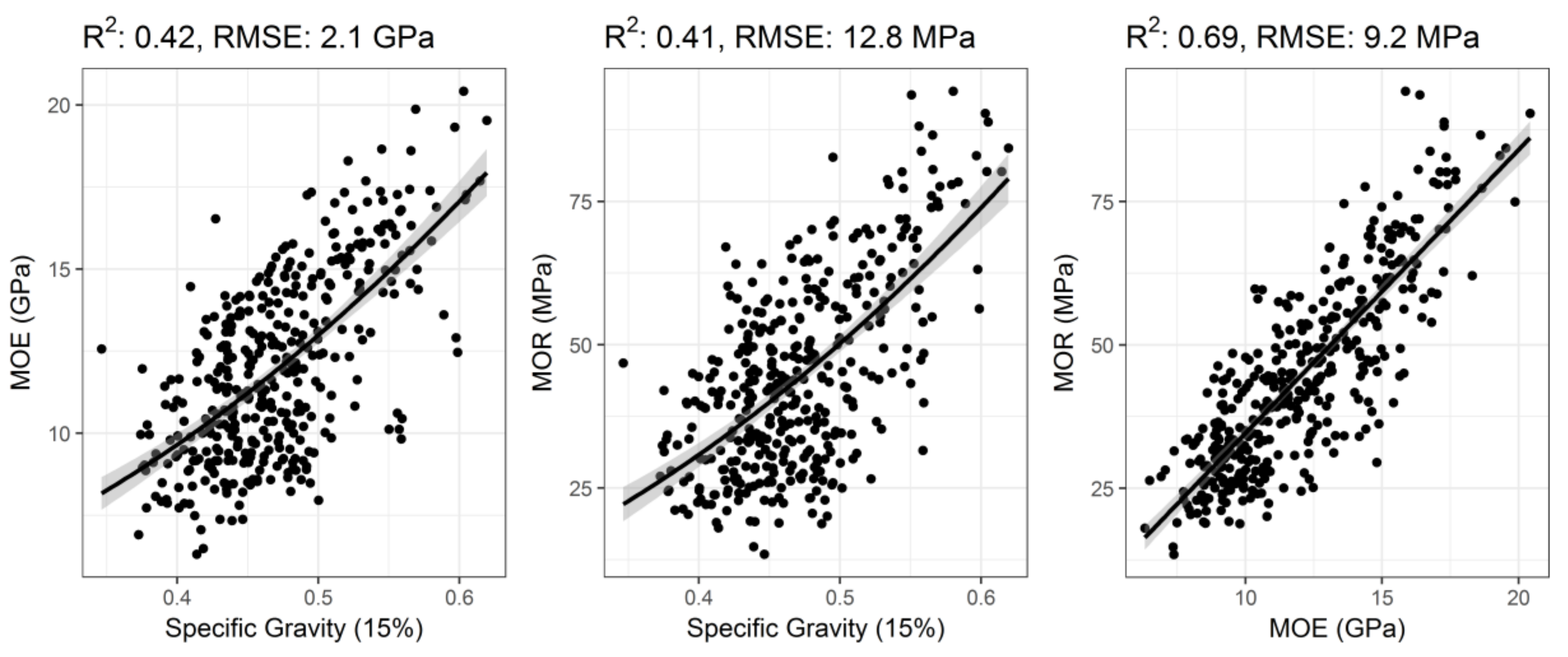
| MOE | 12 | 6.3 | 19.9 | 2.8 | 12 | 6.5 | 20.4 | 2.9 | ||
| MOR | 44.6 | 14.8 | 93.6 | 16.2 | 44.5 | 13.4 | 94.3 | 17.8 | ||
| Calibration | Prediction | |||||||||
|---|---|---|---|---|---|---|---|---|---|---|
| Tool 1 | Property 2 | No. Factors | R2 | SECV | RMSECV | RPDcv | Rp2 | SEP | RPDp | Bias |
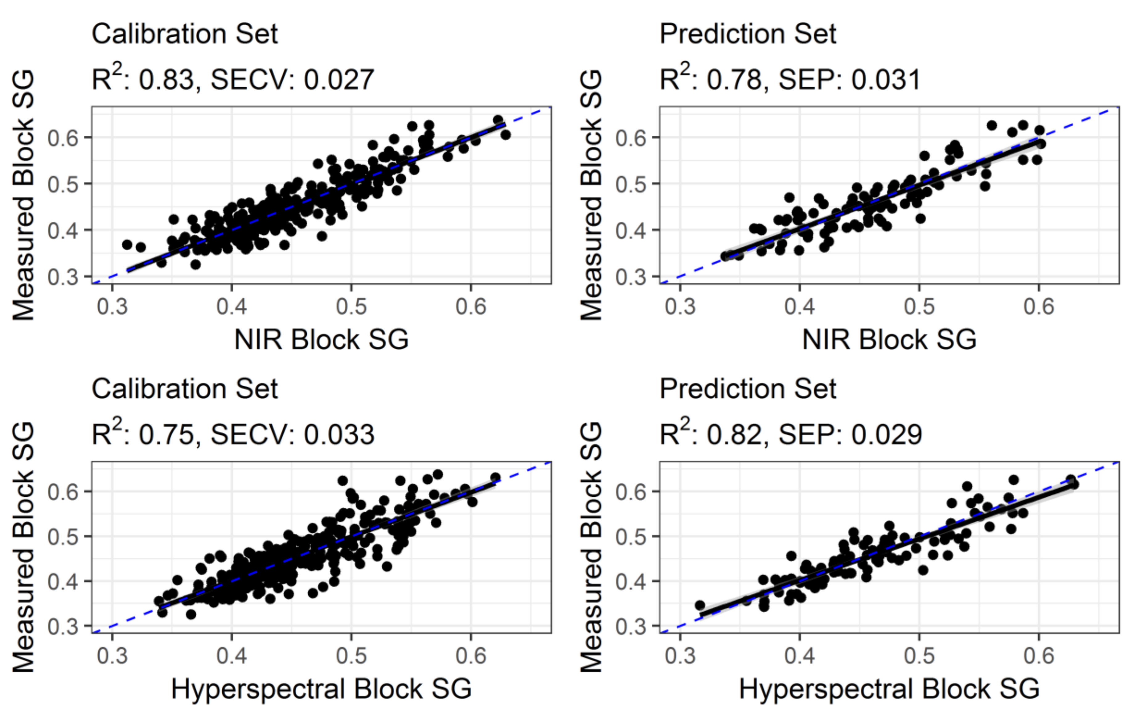
| NIR | SGblock | 10 | 0.83 | 0.027 | 0.035 | 2.4 | 0.78 | 0.031 | 2.1 | 0.00075 |
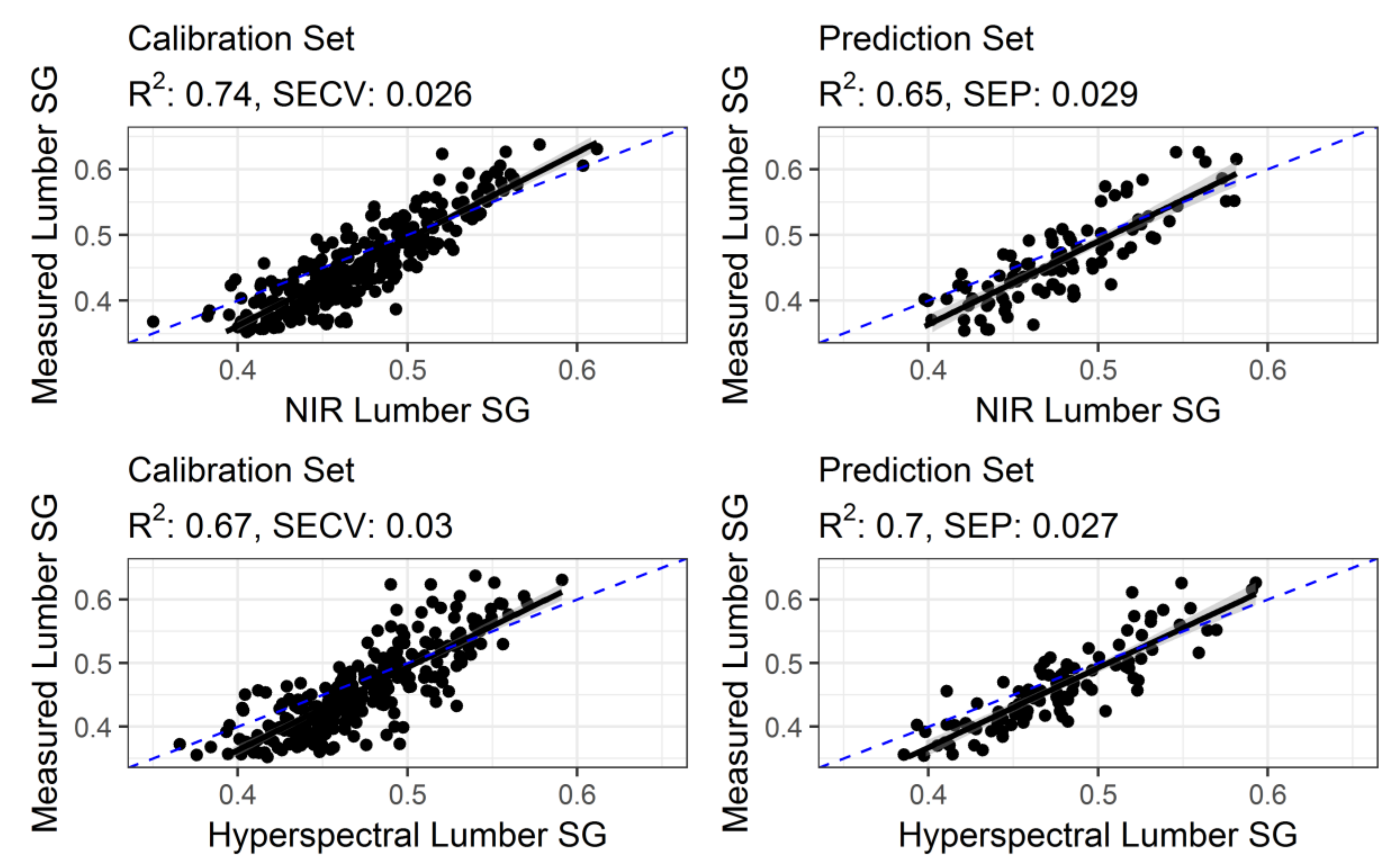
| SGlumber | 10 | 0.74 | 0.026 | 0.032 | 2.0 | 0.65 | 0.029 | 1.7 | 0.0033 | |
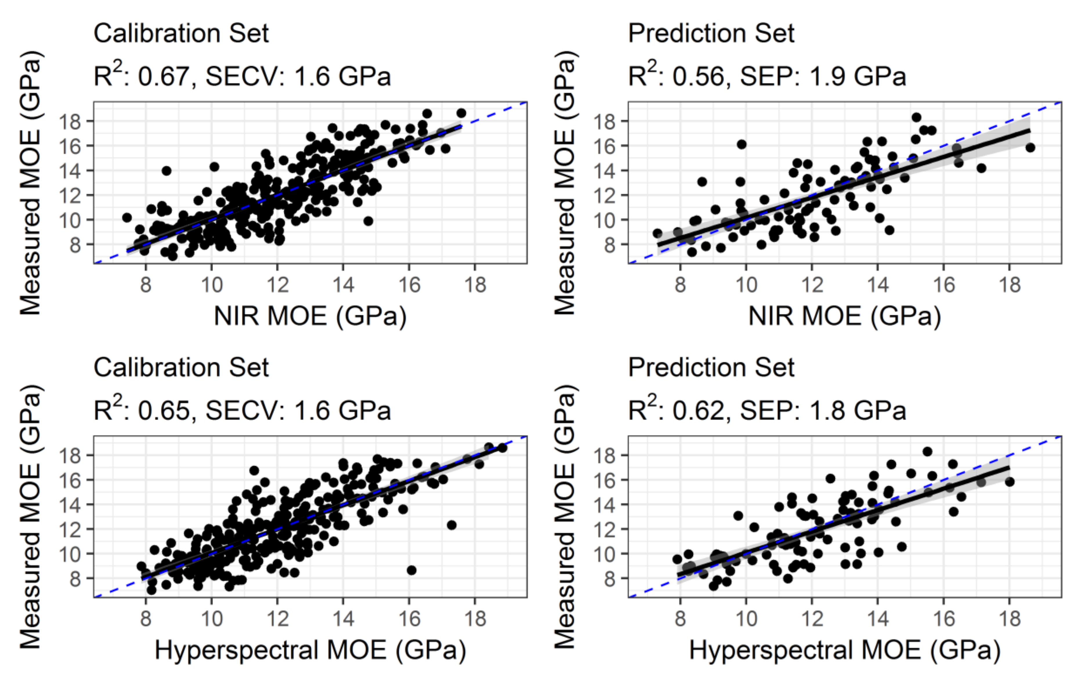
| MOE | 6 | 0.67 | 1.6 | 1.8 | 1.7 | 0.56 | 1.9 | 1.5 | 0.16 | |
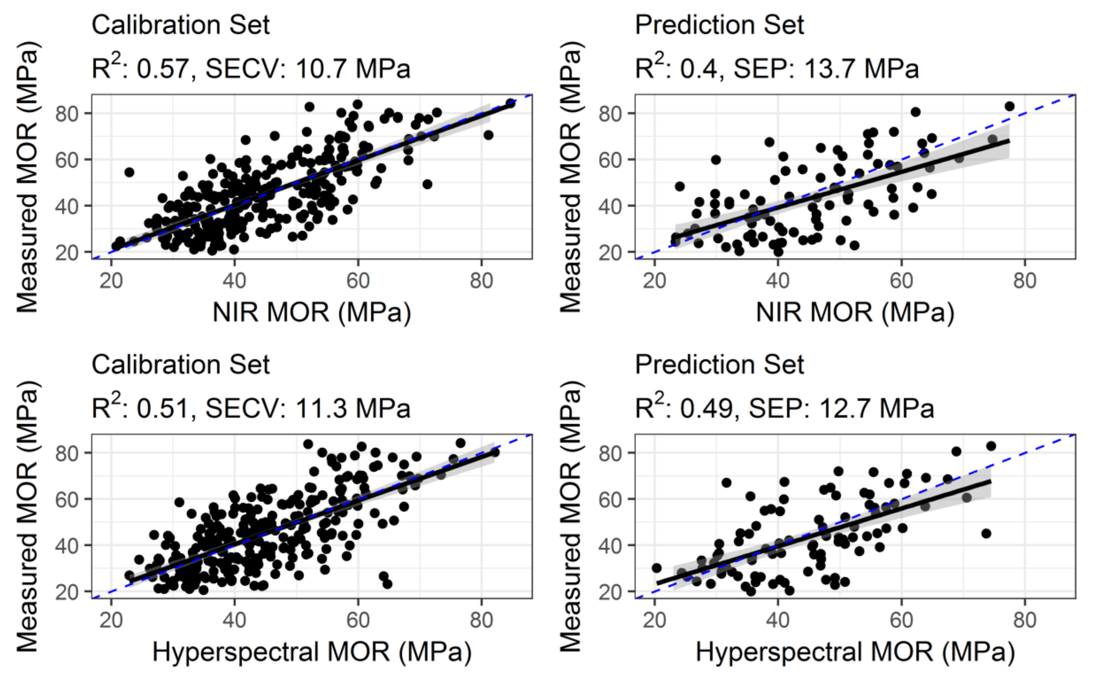
| MOR | 7 | 0.57 | 10.7 | 12.2 | 1.5 | 0.40 | 13.7 | 1.3 | 0.75 | |
| NIR-HSI | SGblock | 6 | 0.75 | 0.033 | 0.037 | 2.0 | 0.82 | 0.029 | 2.3 | 0.0029 |
| SGlumber | 7 | 0.67 | 0.03 | 0.033 | 1.7 | 0.70 | 0.027 | 1.8 | 0.0013 | |
| MOE | 5 | 0.65 | 1.6 | 1.7 | 1.7 | 0.62 | 1.8 | 1.6 | 0.15 | |
| MOR | 6 | 0.51 | 11.3 | 12.2 | 1.4 | 0.49 | 12.7 | 1.4 | 0.79 | |
© 2018 by the authors. Licensee MDPI, Basel, Switzerland. This article is an open access article distributed under the terms and conditions of the Creative Commons Attribution (CC BY) license (http://creativecommons.org/licenses/by/4.0/).
Share and Cite
Schimleck, L.; Dahlen, J.; Yoon, S.-C.; Lawrence, K.C.; Jones, P.D. Prediction of Douglas-Fir Lumber Properties: Comparison between a Benchtop Near-Infrared Spectrometer and Hyperspectral Imaging System. Appl. Sci. 2018, 8, 2602. https://doi.org/10.3390/app8122602
Schimleck L, Dahlen J, Yoon S-C, Lawrence KC, Jones PD. Prediction of Douglas-Fir Lumber Properties: Comparison between a Benchtop Near-Infrared Spectrometer and Hyperspectral Imaging System. Applied Sciences. 2018; 8(12):2602. https://doi.org/10.3390/app8122602
Chicago/Turabian StyleSchimleck, Laurence, Joseph Dahlen, Seung-Chul Yoon, Kurt C. Lawrence, and Paul David Jones. 2018. "Prediction of Douglas-Fir Lumber Properties: Comparison between a Benchtop Near-Infrared Spectrometer and Hyperspectral Imaging System" Applied Sciences 8, no. 12: 2602. https://doi.org/10.3390/app8122602
APA StyleSchimleck, L., Dahlen, J., Yoon, S.-C., Lawrence, K. C., & Jones, P. D. (2018). Prediction of Douglas-Fir Lumber Properties: Comparison between a Benchtop Near-Infrared Spectrometer and Hyperspectral Imaging System. Applied Sciences, 8(12), 2602. https://doi.org/10.3390/app8122602