Abstract
This paper proposes a new high-precision rotor position measurement (RPM) method for permanent magnet spherical motors (PMSMs). In the proposed method, a LED light spot generation module (LSGM) was installed at the top of the rotor shaft. In the LSGM, three LEDs were arranged in a straight line with different distances between them, which were formed as three optical feature points (OFPs). The images of the three OFPs acquired by a high-speed camera were used to calculate the rotor position of PMSMs in the world coordinate frame. An experimental platform was built to verify the effectiveness of the proposed RPM method.
1. Introduction
A spherical motor can make complex motions of three degree-of-freedom (DOF) with its simple structure, which can be applied to many applications, such as robotics, aerospace and military. It has advantages over traditional three DOF motors, which are composed of several single-DOF [1,2], such as low manufacturing cost and high efficiency. Many researchers have studied and developed different kinds of spherical motors. For example, a spherical induction motor was developed by Williams and Laithwaite as early as 1959 [3]. Lee et al. developed a spherical stepper wrist motor based on the principle of variable reluctance spherical motor [4]. Son et al. studied the control methods and working characteristics of a spherical wheel motor [5]. A permanent magnet spherical motor (PMSM), with variable pole pitch and 96 stator poles, was proposed by Kahlen et al. [6]. Chirikjian et al. studied the kinematic design and commutation of a spherical stepper motor [7]. A three-DOF cylindrical spherical ultrasonic motor was developed by Takefumi et al. [8]. The research topics that encompass the field of spherical motors include structural design, magnetic field analysis, rotor position measurement, control strategy, and drive circuit design. Rotor position measurement is a necessary precondition that must be taken into account when attempting to achieve precise control of spherical motors.
Rotor position measurement (RPM) in spherical motors is necessary when considering rotation angles in three directions. It is much more complicated than the RPM in traditional single-DOF motors when only one rotation angle needs to be calculated. Many multi-DOF RPM methods have been proposed, which are generally divided into contact type and non-contact type methods. The contact type method adds a mechanical detection mechanism to the rotor [9,10,11,12,13,14]. This type of the RPM can achieve high-precision results, but the heavy structure of the RPM system increases the moment of inertia to the rotor and brings huge friction resistance to the bearings. In order to avoid extra moment of inertia and friction resistance, the non-contact type method has been put forward to measure rotor position. A non-contact RPM method based on a photoelectric sensor has been proposed by Lee et al. [14,15,16,17]. Garner et al. have proposed a non-contact RPM method based on machine vision [18]. Both mothods provide high-precision results by increasing the density of the grid pattern, but it is difficult to ensure clear grid pattern on the spherical shell when the spherical motor is moving. A non-contact laser-based orientation RPM method has been proposed by Yan et al. [19]. This method is capable of achieving high-precision results, but the bulky structure makes it difficult to be installed in spherical motors. Hall-effect sensors have been used to measure the rotor position for spherical motors [20,21,22,23,24,25,26,27,28], however the magnetic field varies so slowly that the signal induced in the Hall-effect sensor cannot be used to differentiate different rotor positions with high precision. In addition, the terrestrial magnetic field may influence the Hall-effect sensor, leading to a large error in the RPM.
Given the limitations and trade-offs observed from the existing techniques, a novel high-precision non-contact RPM method based on machine vision is proposed for PMSMs in this paper. A LED light spot generation module (LSGM) was installed at the top of the rotor shaft in a spherical motor to form three optical feature points (OFPs). A high-speed camera was used to obtain the images of these three OFPs to compute rotation angles in three directions through image processing, obtaining the rotor position of PMSMs. Compared with other non-contact RPM methods, the proposed method provided reliable and accurate RPM with a simple structure. It was not affected by the environmental field or the moving surface of spherical rotors and, as such, is suitable for other types of spherical motors.
The remaining content of this paper is organized as follows. Section 2 presents the structure of a PMSM. Section 3 introduces the composition of the measurement device, and the principle of the proposed RPM method. Section 4 shows the experimental results for validation of the proposed RPM method. Conclusions are summarized in Section 5.
2. Structure of a PMSM
The structure of a PMSM used in this paper [29] is shown in Figure 1. The PMSM consists of two parts: A spherical rotor and a spherical-shell stator. The radius of the rotor is 65 mm, and the length of the rotor shaft is 40 mm. There are 40 NdFeB permanent magnets on the spherical rotor, which are divided into four layers symmetrically distributed around the equatorial plane of a rotor. 24 air-core coils are assembled on the spherical-shell stator, which are divided into two layers and evenly distributed on both sides of the equator.
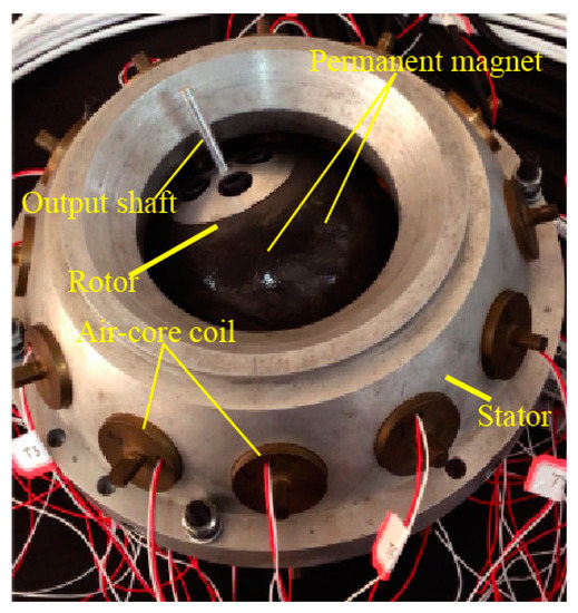
Figure 1.
Structure of the PMSM
Figure 2 shows three-DOF motion of a PMSM. Figure 2a shows the motion range of three-DOF PMSM’s rotor shaft. A stator coordinate frame (SCF) and a rotor coordinate frame (RCF) are used in a PMSM to describe the motion of a spherical rotor. The SCF is stationary relative to the earth, and the center of sphere is defined as the origin (O). The RCF also defines the center of sphere as the origin (o). The centers of the SCF and RCF are completely coincided at the initial position. Figure 2b,c shows the spinning motion and tilting motion of a PMSM, respectively.
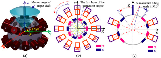
Figure 2.
Three degree-of-freedom (DOF) motion of a permanent magnet spherical motor (PMSM): (a) Rotor shaft motion and the coordinate frames; (b) spinning motion; (c) tilting motion.
3. Rotor Position Measurement for a PMSM
3.1. The Structure of the Measurement Device
Figure 3 shows the structure of the RPM device for the PMSM, which consists of two parts: A high-speed camera and a LED LSGM. The LSGM was installed at the top of the rotor shaft. The distance between the bottom of the rotor shaft and the top surface of the LSGM is 90 mm, and the distance between the lens of the high-speed camera and the top of the LSGM is .
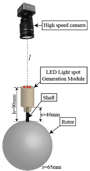
Figure 3.
Schematic diagram of rotor position measurement.
Three LEDs were installed at the top surface of the LSGM, which were arranged in a straight line, as shown in Figure 4. The LED is located at the center, the distance between and was 7 mm and the distance between and was 10 mm. The three optical feature points (OFPs) were identified through the different distances between them. The three LEDs are represented by , , and in the image coordinate frame (ICF), respectively.
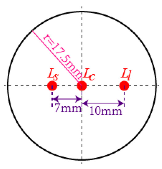
Figure 4.
Arrangement of three LEDs on the top surface of light spot generation module (LSGM).
The parameters of the high-speed camera are shown in Table 1.

Table 1.
Parameters of the high-speed camera
Figure 5 shows the images of three OFPs photographed by the high-speed camera at different exposure times. It can be seen that, when the exposure time of the high-speed camera was 5000 μs, only three OFPs in the image could be identified, which brought great convenience to the subsequent image processing and could be used to extract the coordinates from the three light spots in the ICF.
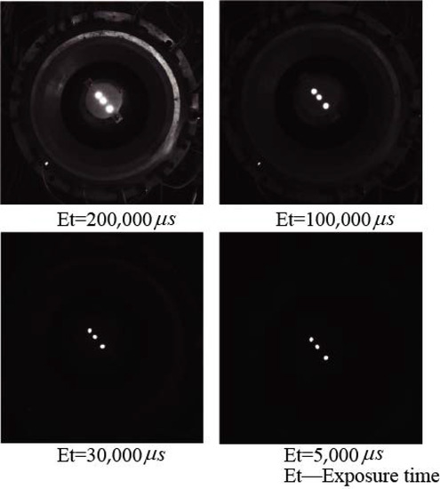
Figure 5.
Images taken by a high-speed camera at different exposure times.
3.2. The Principle of Camera Imaging Based on Pin-Hole Model
A pin-hole model is often used to establish the mathematical model of images in machine vision, which is shown in Figure 6.
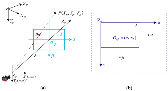
Figure 6.
Pin-hole model in machine vision: (a) Camera pin-hole model; (b) Image coordinate system.
In Figure 6, the point represents the optical center of the camera, and , , , and form the camera coordinate system (CCF). The ICF includes an imaging plane , the horizontal ordinates , and , which are parallel and the vertical ordinates and , which are parallel too, and the optical axis of camera , which is vertical to the imaging plane. The intersection of the optical axis and the imaging plane is the origin of the ICF, which is expressed as . The distance between and is , which is the focal length of the camera. A point in the imaging plane can be expressed as:
where is the coordinate values of , and is the pixel size of the camera.
We define a world coordinate frame (WCF) which constitutes , , and to describe the position of the camera in the CCF. The transformation relationship between the WCF and CCF can be expressed as:
where: is a rotation matrix of ; is a translation vector of ; is a external parameter matrix of .
As observed from triangulation in Figure 6, we can get
Equation (3) can be expressed in the form of matrix as:
Substituting Equations (1) and (2) into Equation (4) leads to
where: , ; is the intrinsic parameters matrix of a camera, which is determined by 、 、 and ; is the extrinsic parameters matrix of a camera, which is determined by the relationship between the CCF and WCF. Equation (5) can be used to calculate the position of objects, such as rotor position in this study. In the following analysis and experiments, the high-speed camera was fixed on a tripod and its distance to the top of LSGM was , which was the main parameter in the experiments.
3.3. Analysis of Rotor Motion in a PMSM
When the PMSM was working in the maximum motion range of three-DOF with the maximum tilting angle of 37.5°, the output shaft tip of the rotor produced a spherical trajectory (gray color) and the midpoint LED in the LSGM also produced another spherical trajectory (red color), as shown in Figure 7. The sphere centers of the two trajectories were the same, the two tilting angles were also the same, but the radii of them were different. Therefore, the spherical trajectory generated by the midpoint LED could be used to determine the position of the rotor shaft.
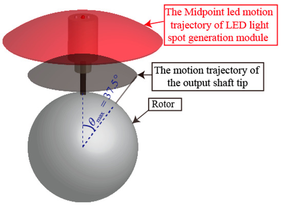
Figure 7.
Rotor motion range of a PMSM.
3.3.1. Calculation of the Rotor Position in a PMSM
The rotor position in a PMSM can be represented by three rotation angles: The tilting angle_, the yaw angle_, and the spinning angle_. Three rotation angels can be calculated by computing the coordinate values of three OFPs in the ICF, which are captured by a high-speed camera. Figure 8 shows the procedure to calculate the three rotation angles.
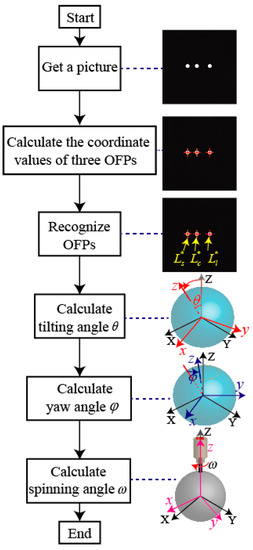
Figure 8.
The procedure to calculate three rotation angles for rotor position in a PMSM.
3.3.2. Calculation of the Tilting angle_
When the tilting angle of the rotor shaft is , Figure 9 shows the relationship between the camera and the midpoint LED, where R is the distance between the sphere center and the midpoint LED.
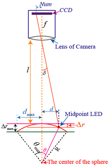
Figure 9.
Calculation of the tilting angle_.
When , i.e., the rotor shaft is perpendicular to the horizontal plane, the distance between the lens of high-speed camera and the midpoint LED is . When varies between 0° and 37.5°, the angle can be computed by
where and are the deflection distances in the horizontal and vertical directions, respectively, is the pixel coordinate distance in the ICF.
Substituting Equations (6) and (7) into Equation (8) yields
Then, the tilting angle is
3.3.3. Calculation of the Yaw angle_
When the rotor moves within the maximum angle, the high-speed camera captures the image of the three OFPs, which are located within a circle at the radius of (the value of is correlation with the experimental parameters), as indicated in Figure 10.
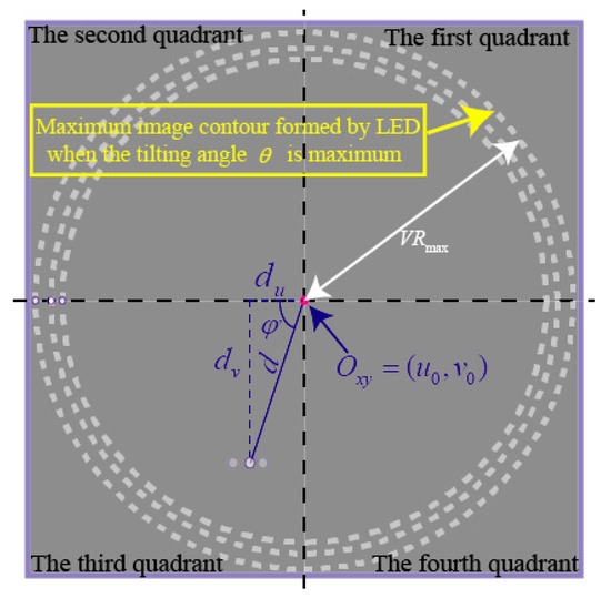
Figure 10.
Calculation of yaw angle_.
Similarly, the angle can be computed by
where: and are the distances between the midpoint LED and the origin in the ICF.
With the calculated , the tilting angle_ in the range of 0~2π can be expressed as:
Thus, the rotor position expressed by the tilting angle_ and yaw_ in a spherical coordinate frame can be converted to a position [, , ] in a rectangular coordinate frame as
where is the distance between the tip of the rotor shaft and sphere center.
3.3.4. Calculation of the Spinning angle_
While the rotor shaft moved within the maximum angle, the rotor was spinning around z axis in the RCF as shown in Figure 11 and the spinning angle is needed to determine the rotor position.
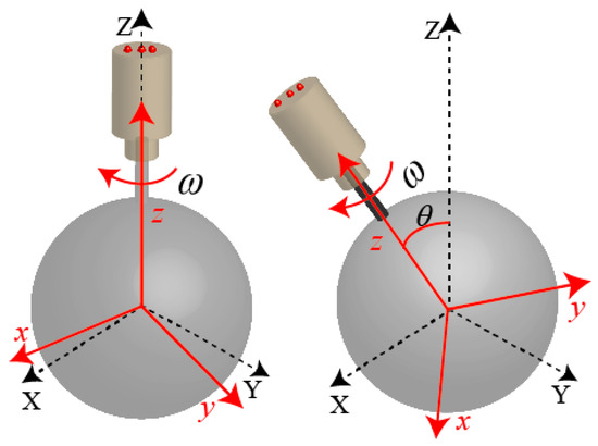
Figure 11.
Spinning motion of the rotor.
Figure 12 shows the images of the three OFPs taken by the high-speed camera when the rotor shaft was spinning.
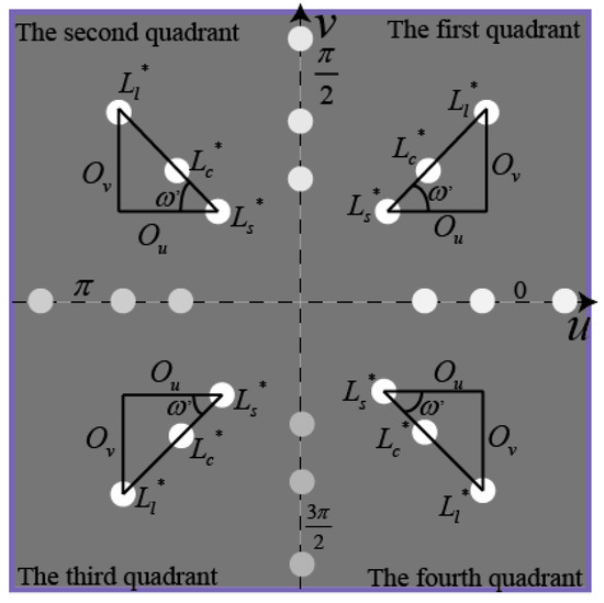
Figure 12.
Images of three optical feature points (OFPs) for calculation of spinning angle_.
The angle can be computed by
where is the distance between and in the direction of axis, and is the distance between and in the direction of axis.
With the rotation angle , the spinning angle_ in the range of 0~2π can be expressed in the four quadrants as:
4. Experimental Results
According to the proposed method, the tilting angle_, the yaw angle_, and the spinning angle_ can be calculated to determine a rotor position of the PMSMs. In order to verify the RPM method for PMSMs, an experimental platform, as shown in Figure 13a, was constructed, which consisted of a PMSM and its control circuit, a LSGM and its driver circuit, a high-speed camera (Revealer, Hefei, Anhui, China) and tripod, a power supply (Tradex, Beijing, China), and a computer (Lenovo, Beijing, China). Figure 13b shows the block diagram of the control system. The block diagram of the rotor position measurement system is shown in Figure 13c.
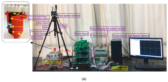
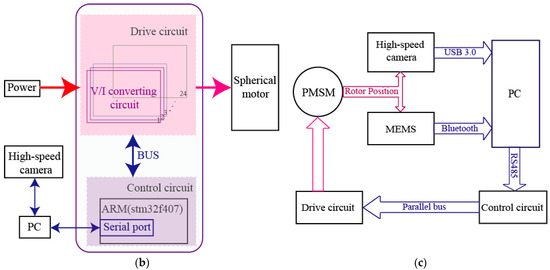
Figure 13.
Experimental platform for measuring the position of the PMSM rotor: (a) Experimental prototype; (b) Block diagram of the control system; (c) Block diagram of rotor position measurement system, micro-electro-mechanical system(MEMS): MPU6050.
Table 2 shows the parameters of the spherical motor driver circuit.
Table 2.
Parameters of the spherical motor driver circuit.
In the following experiment, we set the resolution, the sampling time, and the exposure time of the high-speed camera as 1100 1100, 20 ms and 5000 μs, respectively. The distance between the LSGM’s tip and high-speed camera lens was 420 mm, we can measure through Equation (11) that the maximum value of is 42°, (the maximum tilting angle of PMSM is 37.5°). Consequently, the intrinsic parameter matrix of the camera generated by the calibration method [30] is
From Table 1, , the focal length of the camera can be computed as:
Measurement results obtained by the MEMS were set as the reference (analytical results), Table 3 shows the parameters of the MEMS. Although MEMS can get a precise position of PMSM in a certain time (about 10 min) after calibration, it is known that the measurement error will gradually increase after a certain time. Every measurement time was 10 s in the following experiment.
Table 3.
Parameters of the MEMS.
4.1. Experimental Measurement on Tilting Motion of PMSM Rotor
The rotor shaft can make a tilting motion with respect to the z axis in the SCF, the tilting angle varied between 0° to 37.5°. The initial position was determined by drawing two lines on the stator shell and spherical rotor, respectively, as shown in Figure 14.
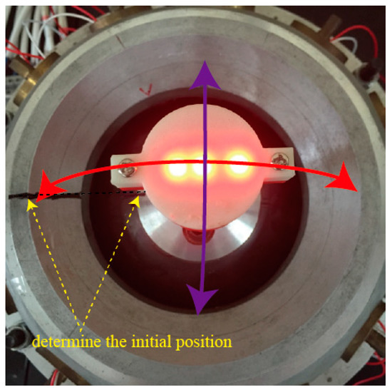
Figure 14.
Tilting motion of PMSM rotor.
Figure 15a shows the images obtained by the high-speed camera when the rotor made a tilting motion; the coordinate values of three OFPs in the ICF were calculated by image processing. Further, we get the position of rotor output shaft tip by the tilting angle_ through Equation (11) and the yaw angle_ through Equation (13), which is shown in Figure 15b.
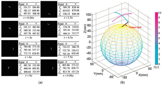
Figure 15.
Experimental measurement on tilting motion: (a) Images captured by high-speed camera and coordinate values of optical feature points; (b) Position of rotor shaft tip.
Figure 16a shows the tilting angle_ when the PMSM made a tilting motion. The maximum tilting angle was about 22°, and the rotor wiggled 11.5 times in 10 s. The maximum difference between the experimental and analytical results of the tilting angle was about 0.32°, as shown in Figure 16b. Figure 16c shows the yaw angle_. It moved between 90° and 270° in the first 5 s, which means the rotor made a tilting motion about 5 times near the XZ plane. In the next 5 s, the rotor made a tilting motion about 6.5 times near the YZ plane and the yaw angle moved between 180° and 360°. The maximum difference between the experimental and analytical results of the yaw angle was about 0.3°, as shown in Figure 16d. Figure 16e shows the spinning angle_. It was about 330° in the first 5 s and was changed into about 255° in the next 5 s. The maximum difference between the experimental and analytical results of the spinning angle was about 0.31°, as shown in Figure 16f.
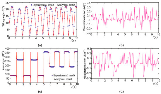
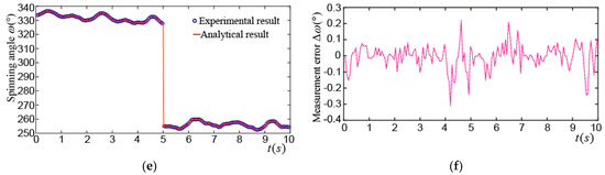
Figure 16.
Experimental results of rotor tilting motion: (a) Experimental and analytical results of ; (b) difference between experimental and analytical results of ; (c) experimental and analytical results of ; (d) difference between experimental and analytical of ; (e) experimental and analytical results of ; (f) difference between experimental and analytical of .
4.2. Experimental Measurement on Spinning Motion of PMSM Rotor at the Center Point
When the rotor was rotating around the z axis at the center point, i.e., the tilting angle_ was 0°, as shown in Figure 17. The spinning angle of the rotor shaft can be calculated from the images which were taken by the high-speed camera.
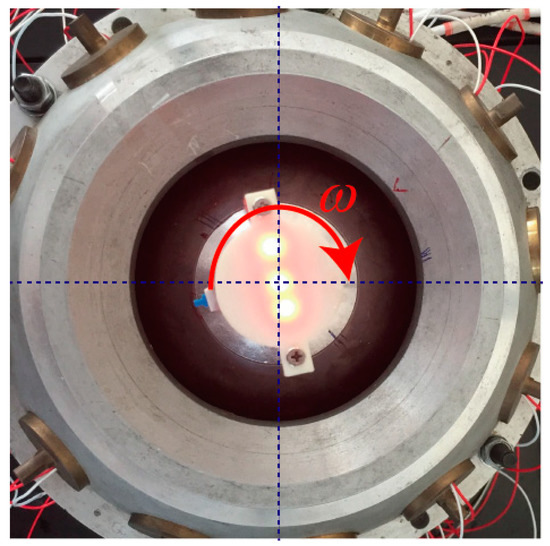
Figure 17.
Spinning motion of PMSM rotor at center point.
Figure 18a shows the images taken by the high-speed camera and the coordinate values of the three OFPs in the ICF. After calculating the tilting angle_ and yaw angle_, we can get the position of rotor output shaft tip, which is shown in Figure 18b.
Figure 18.
Experimental measurement on the spinning motion of PMSM rotor at center point: (a) Images captured by high-speed camera and coordinate values of optical feature points; (b) Position of rotor shaft tip.
Figure 19a shows the tilting angle_ when the PMSM rotor made a spinning motion at the center point, however the maximum tilting angle was about 2.8°. This may be caused by the position direct (PD) control algorithm and the time delay of position detection applied in this PMSM. The maximum difference between the experimental and analytical results was about 0.25°, as shown in Figure 19b. Figure 19c shows the yaw angle_, it varied from 90° to 210°, the maximum difference between the experimental and analytical values was about 0.3°, as shown in Figure 19d. Figure 19e shows the spinning angle_. It can be seen that the PMSM rotor rotated clockwise at about 5.5 turns in 10 s, and the maximum difference between the experimental and analytical values was about 0.3°, as shown in Figure 19f.
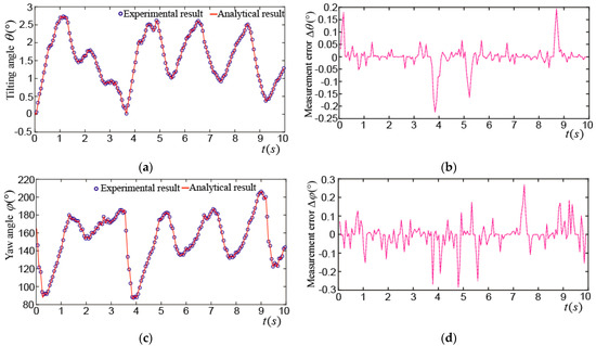
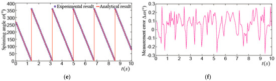
Figure 19.
Experimental results on spinning motion of PMSM rotor at center point: (a) Experimental and analytical results of ; (b) difference between experimental and analytical results of ; (c) experimental and analytical results of ; (d) difference between experimental and analytical of ; (e) experimental and analytical results of ; (f) difference between experimental and analytical of .
4.3. Experimental Measurement on Edge Spinning Motion of PMSM Rotor
Figure 20 shows that the PMSM rotor shaft spinning at a tilted angle. When the rotor shaft was in motion in three-DOF, the spherical rotor span around the tilted z axis at the same time.
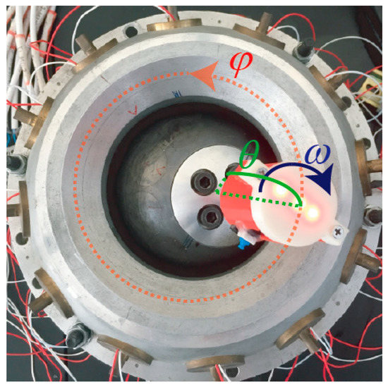
Figure 20.
Edge spinning motion of PMSM rotor.
Figure 21 shows the experimental measurement on the edge spinning motion of PMSM rotor.
Figure 21.
Experimental measurement on the edge spinning motion: (a) Image captured by high-speed camera and coordinate values of optical feature points; (b) Position of rotor shaft tip.
Figure 22a shows the tilting angle_ when the PMSM rotor made an edge spinning motion, its average value was about 24°. The variation of the tilting angle might be caused by the PD control algorithm and the time delay of position detection used in the PMSM. The maximum difference of the tilting angle between the experimental and analytical results was about 0.22°, which is shown in Figure 22b. Figure 22c shows the yaw angle_. It can be seen that the PMSM rotor is rotating anti-clockwise at the approximate 4.5 turns around the z axis in the SCF. The maximum difference of the yaw angle between the experimental and analytical results was about 0.3°, as shown in Figure 22d. Figure 22e shows the spinning angle_, we can see that the PMSM rotor was rotating clockwise at the approximate 4 turns around the z axis in the RCF. The maximum difference of the spinning angle between the experimental and analytical results was about 0.45°, as shown in Figure 22f, this difference was mainly caused by the three LEDs in the LSGM which were not at the same level when the rotor was tilted.
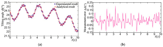
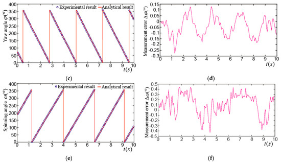
Figure 22.
Experimental results of edge spinning motion of PMSM rotor: (a) Experimental and analytical results of ; (b) difference between experimental and analytical results of ; (c) experimental and analytical results of ; (d) difference between experimental and analytical results of ; (e) experimental and analytical results of ; (f) difference between experimental and analytical results of .
4.4. Comparison of Different Rotor Position Measurement Methods
To date, four types of sensors have been widely used for the RPM including MEMS, photoelectric sensor, Hall-effect sensor, and high-speed camera The experimental results obtained by the MEMS were set as the reference values because the MEMS has been found to have the highest accuracy among four of them. The experimental results obtained by the other three methods were compared with those by the MEMS. Table 4 shows their differences. It can be seen that the high-speed camera based RPM has shown higher accuracy than the other two methods.
Table 4.
Comparison of different rotor position measurement methods.
5. Conclusions
Rotor position measurement (RPM) is a precondition for closed-loop operation of spherical motors. This paper presents a novel RPM method for a PMSM based on image processing. In the proposed RPM, a LSGM was installed at the top of a PMSM rotor shaft, where three LEDs in the LSGM were arranged in a straight line with different distances to form three optical feature points (OFPs). A high-speed camera was used to capture the images of these three OFPs. The coordinate values of the three OFPs in the images were extracted to compute the tilting angle_, the yaw angle_ and the spinning angle_ of the PMSM rotor, and thus obtain the rotor position of a PMSM. As there was no physical contact between a high-speed camera and a PMSM, extra moment of inertia and friction resistance, which may compromise the working performances of spherical motors, were avoided. The experimental platform was set up to verify the effectiveness of the proposed RPM method with high detection precision. In the future, we will install a tiny camera in a PMSM to measure the rotor position, which has negligible influence on the motion of rotor and structure of a PMSM. Combining with the other sensors, we will use the multiple sensor fusion method to further improve the precision of the RPM.
Author Contributions
Y.L. and C.H. designed the architecture of rotor position measurement device, Q.W., W.S. and Y.H. helped the experiments. All of the authors wrote and revised the paper.
Funding
This work is supported by the key project of the China National Natural Science Foundation (51637001).
Conflicts of Interest
The authors declare no conflict of interest.
References
- Glowacz, A. Fault diagnosis of single-phase induction motor based on acoustic signals. Mech. Syst. Signal Process. 2019, 117, 65–80. [Google Scholar] [CrossRef]
- Singh, G.; Naikan, V.N.A. Infrared thermography based diagnosis of inter-turn fault and cooling system failure in three phase induction motor. Infrared Phys. Technol. 2017, 87, 134–138. [Google Scholar] [CrossRef]
- Williams, F.C.; Laithwaite, E.R.; Eastham, J.F. Development and design of spherical induction motors. Proc. IEE Part A Power Eng. 1959, 106, 471–484. [Google Scholar] [CrossRef]
- Lee, K.M.; Vachtsevanos, G.; Kwan, C. Development of a spherical stepper wrist motor. J. Intell. Robot. Syst. 1988, 1, 225–242. [Google Scholar] [CrossRef]
- Son, H.; Lee, K.M. Open-Loop controller design and dynamic characteristics of a spherical wheel Motor. IEEE Trans. Ind. Electron. 2010, 57, 3475–3482. [Google Scholar] [CrossRef]
- Kahlen, K.; Voss, I.; Priebe, C.; Doncker, R.W.D. Torque control of a spherical machine with variable pole pitch. IEEE Trans. Power Electron. 2002, 19, 1628–1634. [Google Scholar] [CrossRef]
- Chirikjian, G.S.; Stein, D. Kinematic design and commutation of a spherical stepper motor. IEEE/ASME Trans. Mechatron. 1999, 4, 342–353. [Google Scholar] [CrossRef]
- Amano, T.; Ishii, T.; Nakamura, K.; Ueha, S. An ultrasonic actuator with multidegree of freedom using bending and longitudinal vibrations of a single stator. In Proceedings of the IEEE Ultrasonics Symposium, Sendai, Japan, 5–8 October 1998; pp. 667–670. [Google Scholar]
- Guo, J.; Kim, D.H.; Son, H. Effects of magnetic pole design on orientation torque for a spherical motor. IEEE/ASME Trans. Mechatron. 2013, 18, 1420–1425. [Google Scholar]
- Sakaidani, Y.; Hirata, K.; Maeda, S.; Niguchi, N. Feedback control of the 2-dof actuator specialized for 2-axes rotation. IEEE Trans. Magn. 2013, 49, 2245–2248. [Google Scholar] [CrossRef]
- Liu, J.; Deng, H.; Chen, W.; Bai, S. Robust dynamic decoupling control for permanent magnet spherical actuators based on extended state observer. IET Control Theory Appl. 2017, 11, 619–631. [Google Scholar] [CrossRef]
- Liu, J.; Deng, H.; Hu, C.; Hua, Z.; Chen, W. Adaptive backstepping sliding mode control for 3-dof permanent magnet spherical actuator. Aerosp. Sci. Technol. 2017, 67, 62–71. [Google Scholar] [CrossRef]
- Zhang, L.; Chen, W.; Liu, J.; Wen, C. A robust adaptive iterative learning control for trajectory tracking of permanent-magnet spherical actuator. IEEE Trans. Ind. Electron. 2015, 63, 291–301. [Google Scholar] [CrossRef]
- Bai, K.; Lee, K.M. Direct field-feedback control of a ball-joint-like permanent-magnet spherical motor. IEEE/ASME Trans. Mechatron. 2014, 19, 975–986. [Google Scholar] [CrossRef]
- Stein, D.; Scheinerman, E.R.; Chirikjian, G.S. Mathematical models of binary spherical-motion encoders. IEEE/ASME Trans. Mechatron. 2003, 8, 234–244. [Google Scholar] [CrossRef]
- Strumik, M.; Wawrzaszek, R.; Banaszkiewicz, M.; Seweryn, K. Analytical model of eddy currents in a reaction sphere actuator. IEEE Trans. Magn. 2014, 50, 1–7. [Google Scholar]
- Rossini, L.; Mingard, S.; Boletis, A.; Forzani, E.; Onillon, E.; Perriard, Y. Rotor design optimization for a reaction sphere actuator. IEEE Trans. Ind. Appl. 2014, 50, 1706–1716. [Google Scholar] [CrossRef]
- Garner, H.; Klement, M.; Lee, K.M. Design and analysis of an absolute non-contact orientation sensor for wrist motion control. In Proceedings of the IEEE/ASME International Conference on Advanced Intelligent Mechatronics, Como, Italy, 8–12 July 2001. [Google Scholar]
- Yan, L.; Chen, I.M.; Guo, Z.; Lang, Y.; Li, Y. A three degree-of-freedom optical orientation measurement method for spherical actuator applications. IEEE Trans. Autom. Sci. Eng. 2011, 8, 319–326. [Google Scholar] [CrossRef]
- Wang, J.; Jewell, G.W.; Howe, D. Analysis, design and control of a novel spherical permanent-magnet actuator. IEE Proc. Electr. Power Appl. 1998, 145, 61–71. [Google Scholar] [CrossRef]
- Li, H.; Liu, W.; Li, B. A sensing system of the halbach array permanent magnet spherical motor based on 3-D hall sensor. J. Electr. Eng. Technol. 2018, 13, 352–361. [Google Scholar]
- Wang, J.; Wang, W. Jewell, G.W.; Howe, D. A novel spherical permanent magnet actuator with three degrees-of-freedom. IEEE Trans. Magn. 1998, 34, 2078–2080. [Google Scholar] [CrossRef]
- Wang, W.; Wang, J.; Jewell, G.W.; Howe, D. Design and control of a novel spherical permanent magnet actuator with three degrees of freedom. IEEE/ASME Trans. Mechatron. 2003, 8, 457–468. [Google Scholar] [CrossRef]
- Jin, H.Z.; Lu, H.; Cho, S.K.; Lee, J.M. Nonlinear Compensation of a New Noncontact Joystick Using the Universal Joint Mechanism. IEEE/ASME Trans. Mechatron. 2007, 12, 549–556. [Google Scholar] [CrossRef]
- Rossini, L.; Chetelat, O.; Onillon, E.; Perriard, Y. Force and torque analytical models of a reaction sphere actuator based on spherical harmonic rotation and decomposition. IEEE/ASME Trans. Mechatron. 2013, 18, 1006–1018. [Google Scholar] [CrossRef]
- Li, B.; Li, Z.; Li, G. Magnetic field model for permanent magnet spherical motor with double polyhedron structure. IEEE Trans. Magn. 2017, 53, 1–5. [Google Scholar] [CrossRef]
- Li, B.; Zhang, S.; Li, G.; Li, H. Synthesis strategy for stator magnetic field of permanent magnet spherical motor. IEEE Trans. Magn. 2018, 99, 1–5. [Google Scholar] [CrossRef]
- Li, H.; Li, T. End-effect magnetic field analysis of the halbach array permanent magnet spherical motor. IEEE Trans. Magn. 2018, 99, 1–9. [Google Scholar] [CrossRef]
- Zhao, L.; Li, G.; Guo, X.; Li, S.; Wen, Y.; Ye, Q. Time-optimal trajectory planning of permanent magnet spherical motor based on genetic algorithm. In Proceedings of the 2017 12th IEEE Conference on Industrial Electronics and Applications (ICIEA), Siem Reap, Cambodia, 18–20 June 2017; pp. 828–833. [Google Scholar]
- Zhang, Z. A Flexible New Technique for Camera Calibration. IEEE Trans. Pattern Anal. Mach. Intell. 2000, 22, 1330–1334. [Google Scholar] [CrossRef]
© 2018 by the authors. Licensee MDPI, Basel, Switzerland. This article is an open access article distributed under the terms and conditions of the Creative Commons Attribution (CC BY) license (http://creativecommons.org/licenses/by/4.0/).