Featured Application
The hydroacoustic setup in this investigation enabled the monitoring of riverine fish in challenging conditions posed by deep, dark and turbulent waters. Specifically, it allowed for the collection of fish position in front of a vertical trash rack at a run-of-river hydropower plant. Information on fish assemblages was furthermore combined with in-situ flow velocity and pressure turbulence data, revealing new insights regarding fish hydrodynamic preferences. The applied combined acoustic-hydrodynamic method can be used to support planning processes as well as the design and monitoring of suitable mitigation measures for downstream fish migration.
Abstract
The spatial distribution of fish upstream of a vertical trash rack was investigated at the hydropower plant Kirchbichl in the alpine River Inn (Tyrol, Austria). The objective of the research project “FIDET” was to establish a non-invasive methodology to study fish presence and flow characteristics at large hydro power sites. A new monitoring approach was developed combining hydroacoustic observations of fish locations with multivariate hydrodynamic data. This was accomplished by utilizing complementary observations from multiple underwater sensor technologies: First, an array of echosounders were deployed at a fixed cross-section upstream of the trash rack for long-term monitoring. Afterwards, detailed underwater surveys with “acoustic cameras” (DIDSON and ARIS) revealed that the spatial distributions of fish in front of the trash rack were highly heterogeneous. The spatial distribution of the flow field was assessed via the time-averaged velocity fields from acoustic Doppler current profiler (ADCP). Finally, a custom pressure-based flow turbulence probe was developed, providing spatial estimates of flow turbulence immediately upstream of the trash rack. The significant contribution of this work is to provide a multi-modal monitoring approach incorporating both fish position data and hydrodynamic information. This forms the starting point for a future objective, namely to create an automated, sonar-based detection and control systems to assist and monitor fish protection operations in near real-time.
Keywords:
fish monitoring; downstream migration; alpine river; EK15; DIDSON; ARIS; differential pressure; turbulence 1. Introduction
European research on downstream migration of fish began some 30 years ago [1,2,3,4], and has increased substantially in the last decade, especially in Germany [5,6,7]. The majority of studies are focused on diadromous fish, such as Atlantic salmon [8,9] and European eel [8,10,11]. Most studies have been limited to small hydropower plants [12,13]. Research on large hydropower plants is therefore needed to develop suitable measures for the full spectrum of European hydropower facilities. Currently, the ongoing discussion on fish protection and downstream migration focuses on three key aspects: (1) The catchment area and its representative target species; for example, the Danube versus the Rhine, where Atlantic salmon and European eel naturally occur only in the Rhine catchment. (2) The biocoenotic region (rithral versus potamal) as alpine waters that have only a few species differ widely from lowland waters, which commonly have >25 species. (3) Differences in the hydropower plant design, especially the turbine size and type. Based on these three aspects, it has been established that a case-by-case examination is necessary to determine the balance between ecological need and economic utility at each hydropower facility [14,15,16].
Currently, there is no best practice concerning the provision of facilities for downstream migration of fish and/or fish protection in Austria [17]. To address this, three research projects are underway. The first is a project on downstream migration at small hydropower plants [18]. Secondly, the project “Downstream fish migration on medium-sized rivers in Austria: population basics and implications for fish protection and fish descent” [19]. And finally, the project “Fish detection and fish behavior: hydroacoustic investigations for the assessment of presence and behavior of fish in front of the trash rack of-run of-river plants” (FIDET). This paper reports the main findings of the third project, FIDET.
The major challenge of in-situ research is to develop practical field measurement methods capable of addressing knowledge gaps. This can be achieved by combining multiple measurement technologies, both in the lab and in the field [20,21,22]. Currently, there are no published datasets on fish presence and behavior in the vicinity of trash racks of large HPPs in the Alpine region, with its potamodromous fish fauna. Thus, the FIDET project was initiated to establish new methodological approaches to assess the presence and behavior of fish in front of trash racks [15,23].
Further, it is important to assess the local flow conditions directly upstream of physical barriers to compare fish presence with the spatial distribution of the time-averaged velocity and turbulent fluctuations. Indeed, it is well-established that the local flow environment can have a strong influence on fish swimming behavior, orientation of movement, act as flow cues, and be strongly related to the swimming speed of fish [24]. While the presence and intensity of flow turbulence is known to affect fish swimming and hydraulic preference [25,26], there is a lack of suitable measuring methodology capable of providing turbulence metrics for field studies. The “Differential Pressure Box” (DBox) was specially developed as part of the FIDET project, and presents a new type of turbulent flow sensing device.
Due to the challenging conditions encountered in the field, we provide one of the few in situ investigations of local hydrodynamic conditions upstream of hydropower intakes [18,27]. We show the potential of combining hydroacoustic and flow field turbulence measurement methods to detect periods with increased fish occurrence as well as to analyze spatial distributions of fish at mechanical barriers at the individual level. We applied a multi-modal fish monitoring method using a case study in the Austrian Alps based on a three-staged approach:
- Seasonal patterns of fish presence in the headrace channel using long-term assessments from single-beam echosounders,
- Observations of fish behavior (spatial distribution) in front of the trash rack with acoustic cameras,
- Assessment of local flow field hydrodynamics via combined time-averaged flow velocity and pressure turbulence measurements.
When combined, the different data sources can provide key parameters to assess the relevance of downstream migration and to develop suitable measures regarding fish passage.
2. Materials and Methods
2.1. Case Study Site
The Austrian hydropower plant (HPP) Kirchbichl on the River Inn was built between 1938 and 1941 as a diversion plant, however, it is operated as a run-of-river power plant [28]. At Kirchbichl an omega-shaped loop of the River Inn, with a length of 3.5 km, is cut off by a ~1 km long headrace channel (Figure 1). In order to increase the fall head of the HPP, the River Inn is impounded to 6 m by a weir at the beginning of the river loop. The HPP utilizes the head difference across the river loop, which varies between 7.5 and 9.7 m, depending on the discharge. Three turbines with a design discharge of 250 m3 s−1 and an output of 19.2 MW generate an average of 130.6 GWh a−1 of electricity. Currently, an extension project is under construction. The extension project was developed on the basis of three complementary goals: (1) To achieve compliance with the EU Water Framework Directive by improving the aquatic ecosystem. This includes the establishment of a minimum residual flow as well as the mitigation of surge (related to upstream hydropower plants) and the establishment of fish passage. (2) Compliance with the EU Floods Directive to improve flood protection at the existing HPP. (3) Following the EU Renewable Energy Directive, the extension project includes a refurbishment as well as an increase of the design flow of the existing HPP. In the future, the extended HPP will have an increased design discharge of 484 m3 s−1 (plus additional 15 m3 s−1 at a HPP for residual flow at the weir). The new total output of ~38 MW will generate about 165 GWh a−1 of electricity. The catchment size of the gauging station Bichlwang is 9310 km2 and an analysis of the time series data from 1985 to 2011 established a mean discharge (MQ) of 293 m3 s−1, a maximal mean discharge (HJMQ) of 374 m3 s−1 (1999), a mean flood event (MJHQ) of 1187 m3 s−1 and a maximal discharge (HQ) of 2454 m3 s−1 (23.08.2015), with typical discharges of ≥400 m3 s−1 in the summer months (May–August).
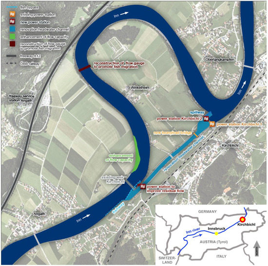
Figure 1.
Overview on the study area, including information on the ongoing extension of the HPP Kirchbichl.
The fish region in this section of the River Inn is assigned to “Epipotamal large” (barbel region); however, due to the presence of glaciers in the catchment, the maximum summer water temperatures are ~15 °C. These characteristics are indicative of an alpine river with a strong glacial influence, which is also reflected in the composition of the fish fauna as well as their biomass. A mean fish biomass of 25.1 kg ha−1 (296 fish ha−1) in the Kirchbichl reservoir and a mean fish biomass of 22.6 kg ha−1 (134 fish ha−1) in the Langkampfen reservoir, located below HPP Kirchbichl, was assessed via a hydroacoustic survey in 2012 [29]. In addition, an electrofishing campaign was carried out in the Kirchbichl reservoir in 2012: with 461 individuals ha−1 accounted for a biomass of 23.4 kg ha−1. In total, only five fish species were detected, and their abundance (brown trout 6.3%, bullhead 6.7%, rainbow trout 77.9%, grayling 2.6% and common nase 6.5%; in % of the total density) indicate that the water body is affected by stocking activities [30]. Within the Austrian national monitoring framework (GZÜV), electrofishing was carried out the river stretch below HPP Langkampfen in November 2008. A total of 14 fish species were found, which represents a wide range for an Alpine catchment. However, the fish density and biomass remained low at 92.1 individuals ha−1 and 5.1 kg ha−1. Based on the aggregation of these findings, the site-specific conditions regarding fish downstream migration can be summarized as follows: (1) The target species are potamodromous fish. (2) Due to the alpine catchment, the number of species is low and also fish biomass is comparatively low [23]. Over the last centuries, multiple hydromorphological pressures have been documented, including land reclamation, flood protection, the establishment of civil transportation infrastructure (e.g., railway, motorway) as well as hydropower development. Accordingly, the River Inn has been classified as a heavily modified water body in the Austrian province of Tyrol [17].
2.2. Long-Term Assessment Using Echosounders
In order to analyze seasonal patterns of fish presence in the headrace channel and identify optimal deployment times for the multibeam systems, fixed location echosounders were used for long term assessment. Data collection was carried out over 13 months from February 2015 to March 2016. Three Simrad EK15 single-beam echo sounders (Simrad A/S, Horten, Norway) with a frequency of 200 kHz and an opening angle of 28° [31], were mounted on floats to detect temporal occurrence of fish in the headrace channel [32]. The floats were manufactured polyester-coated styrofoam bodies with mounting space for the transducer and mounting points. The three units were placed approximately 200 m upstream of the trash rack, covering the majority of the channel width. This location was selected due to suitable flow conditions; i.e., the low acoustic noise level. The floats were held in place using a double rope assembly. An upstream cable assembly was used for deployment and to fix the position of the floats. A second cable, located some six meters downstream was used to lift the floats from the surface during times of high water, in the presence of large floating debris and drifting ice. The use of the three parallel echosounders enabled a large volume of the channel to be sampled with only the embankment zones missed (Figure 2). Despite the occurrence of some blind spots (unsampled regions), the setup ensured a constant sampling volume. The three echosounders were connected to each other via the EK15 software and controlled sequentially every 50 ms, which corresponds to approx. 7 pings per second per channel. This was done to exclude mutual interference or “cross-talk”. Raw data was collected with a pulse length of 80 μs at a threshold of −70 dB. The systems were calibrated separately “on-axis” using the procedure provided by the manufacturer (Simrad EK15, Reference manual / Interactive version, Release 1.2.4, 2014). Exact information on the near-field of the 200-28 CM-transducer was not provided in the manual. However, the first meter of the water column remained unconsidered for analysis to avoid potential near-field effects. Remote access to the echosounders allowed a continuously monitored data acquisition via LAN connection.
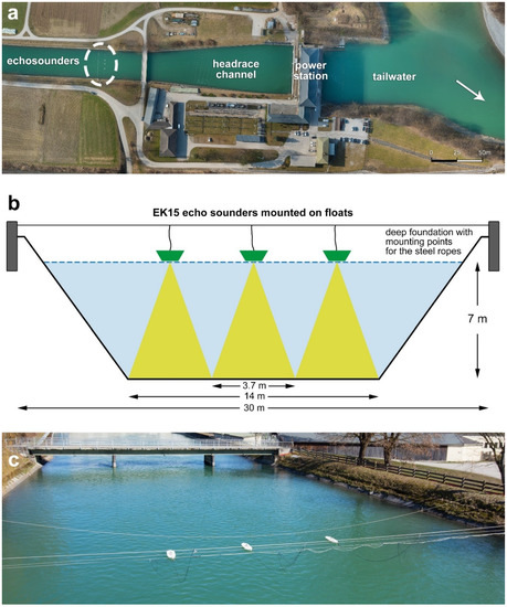
Figure 2.
Overview of the headrace channel with the installation of the EK15 sounders indicated, the power station itself and the tailwater (a) Plan view using an orthoimage of the site (photo: droneproject.at). (b) Schematic cross-section through the headrace channel, showing the setup of the EK15 echosounders. (c) Image of the installation, facing into flow direction.
The echosounder data was post-processed using the software Sonar 5 Pro (Cage Eye A/S, Oslo, Norway). The raw data collected in the field are first converted (Figure 3a). The amplitude (AMP) echograms display the digitized sample data for each ping, whereas the single echo echograms (SED) contain only the individual echoes that were detected. From individual echoes (based on threshold parameters) a fish echo track can be generated (Figure 3b). To determine the threshold parameters, detection experiments were first carried out using stocked rainbow trout of two known size classes (15–18 and 25–30 cm). The fish were released in close range to the echo sounder in small groups over a period of three hours.
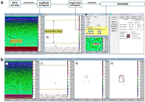
Figure 3.
EK15 echosounder post-processing workflow. (a) The raw data files are converted to amplitude echograms (AMP) and single echo detection echograms (SED). The selected region (examination layer) is analyzed using an automated tracking algorithm. (b) The fish tracking process: (I) Fish target determination in the AMP-echogram. (II) Identification of the same fish target in the SED echogram. (III) Single echoes of the fish target over time. (IV) The completed track by with connecting single echo location. Note that three single echoes were not included in the track, as they did not match the tracking criteria and were not considered.
Tracking tests formed the basis for all echosounder data analyses: all 112 manually detected and evaluated fish echoes or tracks had target measures in the range from −40 to −56 dB with an average of −48.2 dB. The number of individual echoes per track was at least ten and was a maximum of 37 echoes per track (Figure 4). The maximum distances of the individual echoes within each track (i.e., the vertical extent of a track in the water column) were between 0.05 and 0.82 m with a mean of 0.14 m. Based on these evaluations and the observed signal to noise ratio, the field data assessment and subsequent post-processing threshold was set to −50 dB. The minimum number of individual echoes per track was set at twelve; i.e., every track included at least twelve consecutive individual echoes.
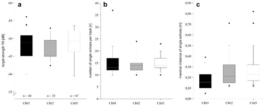
Figure 4.
Results (box plots: line = median, black dots = outliers) from the fish detection test for each of the three channels (Ch01 = right, Ch02 = middle position, Ch03 = left). (a) target strength TS [dB]; (b) number of single echoes per track [n]; (c) maximal distance of single echoes [m].
2.3. Detailed Investigation of Fish Behavior
DIDSON (Dual-Frequency Identification [33]) and ARIS (Adaptive Resolution Identification [34]) sonars, which produce video-identical image sequences, represent the state of the art technology in the field of visualization sonars and are often referred to as “acoustic cameras” [35]. The technology is most commonly used in dark and turbid waters where optical systems cannot capture meaningful data. Their applications are diverse and allow for the direct observation and recording of fish migration, fish behavior near migratory barriers, cooling water withdrawals, hydroelectric plants, bypass systems, spawning grounds, natural and artificial structures and fishing equipment [9,36,37,38,39,40,41].
The imaging properties of DIDSON and ARIS are principally determined by their operating frequencies, which range from 0.7 to 3.0 MHz [42]. The multibeam opening angle is typically 14° (vertical) and 29° (horizontal) and the number of single beams forming the array is a function of the operating frequency, varying between 48 and 128 single beams. The range of the projected sound cone depends on the frequency and varies from a few meters to >20 m for long range applications [43]. This allows for the two-dimensional detection of fish and other underwater objects. Depending on the application and the recording settings, the multibeam sonar used in this work can capture up to 16 images per second. This high rate of recording facilitates the recording of sonar video. The frame rate depends on the device frequency and the site-specific acoustic conditions. In this study a range of 8–12 frames per second (fps) for the DIDSON and 10–16 fps for the ARIS were achieved. The raw data files (.ddf or .aris, respectively) were stored on mobile hard drives for further transfer and processing.
To record the sonar data in front of the trash rack of the HPP Kirchbichl, an innovative setup was developed, taking into accounts the simultaneous use of three imaging sonars (Figure 5a). Two DIDSON sonars (DIDSON 300 with 1.8 MHz) were positioned in front of the trash rack on the left and right bank by means of a rail mounting for depth adjustment (Figure 5b). The ARIS (ARIS 3000 with 1.8 MHz) was mounted on the provided scrape cleaner and/or jib and could thus move along the trash rack at six horizontal positions (Figure 5c). The use of both sonar systems mainly had two advantages, i.e., practical setup performance but furthermore the chance for higher resolution data. De-mounting one of the DIDSONs for the trash rack setup was unnecessary due to availability of the ARIS and thus both systems could be left at their mountings during the whole survey. While the resolution of the DIDSON is always limited to 512 range bins per frame, the ARIS range resolution is adaptive and delivered 2000 samples for the given range setting. Gathering such high-resolution data to evaluate potential of the ARIS in this novel setup was a crucial technical aspect of this study.
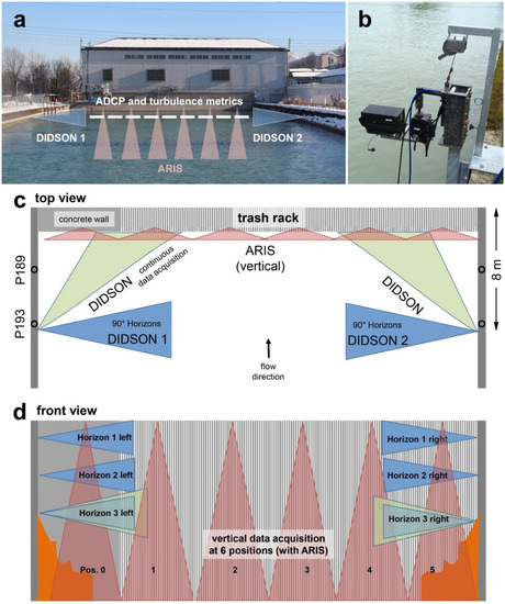
Figure 5.
Hydroacoustic imaging setup with DIDSON and ARIS sonar systems in front of the trash rack: (a) Overview of site. (b) DIDSON. (c) Plan view (the DIDSON were installed close to profile 193, approximately 8 m from the uppermost edge of the inclined trash rack). (d) Front view (orange = sediment deposits in front of the trash rack). The vertical trash rack is inclined at an angle of 70°; i.e., when measured from the top of the trash rack, the bottom of the trash rack ends at the river bed 4 m in the upstream direction.
The first data collection took place from 6–10 September 2016 (>170 h sonar data). Despite favorable acoustic conditions, no fish contacts were recorded during this period. The second data collection took place in the period 4–8 April 2017, corresponding to earlier long-term monitoring results that indicated increased fish presence in the spring [15,23]. Overall, the data from spring 2017 covers a total period of >170 h sonar data (Table S1): The data collection in the horizons 1–3 with a 90° angle from the shore and a window length of 10 m (Figure 5d) were carried out in parallel with two devices, and twice a day for 15 min per horizon during three consecutive days (9 h sonar data). Although originally planned, data acquisition deeper in the water column was not possible due to sediment deposits on the side walls (Figure 5d). During the rest of the time (day and at night) the two sonars, located at the left and right bank were used to continuously record data in the 3 m depth (horizon 3) at a 45° angle towards the trash rack (81 h sonar data from each DIDSON).
The vertical data collection was carried out from d 5–7 April 2017 once a day in six positions (0–5) along the 45 m wide trash rack and ten minutes per position from one meter below the water surface to the bottom. The position 0 corresponds to the starting point on the left bank and the position 5 to the end point at the right bank (Figure 5d). During the vertical data collection, the DIDSON sonars were turned off, in order to eliminate interference. The analyses of the data, which included an assessment of fish contacts, were carried out in depth steps of 0.5 m water columns.
The sonar data were post-processed with the Sonar 5 Professional software package (version 6.0.4; Cage Eye A/S, Oslo, Norway) and ARISFish (version 2.1; Sound Metrics, Bellevue, USA). In ARISFish the echogram mode was used to identify fish echoes and measured in the video playback window of the software. No file-shortening processes were used prior to the analysis. Records from the horizons and the vertical setup were analyzed completely. The continuous records (horizon 3; 45° angle towards the trash rack) were analyzed in sub-samples of 15 min per recorded hour, in the last quarter of each full hour. Every fish inside the sound cone represented a fish contact. However, as fish swam into and out of the sound cone and may re-enter several times, multiple contacts of the same fish during the observation period are highly probable. Thus, absolute quantification was not possible. However, the observation did provide clear probabilities and information on fish behavior and spatial distribution. In addition to the fish contact numbers, we assessed the length of the detected individuals by measuring a back-bone poly-line [44]. Every frame was checked and the one showing the best image was used for measuring along with their position in the sound cone.
2.4. Flow Field Hydrodynamics
In addition to fish position estimates using sonar, our aim was to compare these estimates with in situ measurements of the flow field. This required the development and testing of a new device and method for turbulent flow measurements needed for in situ studies of down-stream migration. To achieve this, we developed a new pressure-based field probe for flow turbulence measurement (“Differential Pressure Box”; DBox). The device is based on the Fechheimer Pitot concept [45], which the authors have successfully developed and tested extensively for underwater vehicles [46,47]. It was designed and implemented for application in rivers with highly turbulent flows ranging from 0 to 3 m/s, and calibrated using in situ ADCP measurements [48]. The combination of spatially explicit, time-averaged flow velocities recovered from ADCP in conjunction with the DBox differential pressure turbulence measurements thus form a spatially resolved, dynamic picture of the complex flow field experienced by fish in front of hydropower intakes.
Estimation of the time-averaged flow velocity as well as its fluctuations caused by turbulence are achieved using the optimized, Fechheimer arrangement of the pressure sensors; the differential pressure is measured at the nose at the stagnation point where velocity goes to zero, and kinetic energy is transferred into pressure. In addition, two pressure ports are located at 35° to the left and right of the stagnation point, which correspond to the locations of local hydrostatic pressure on a cylindrical surface (Figure 6a). The relationship (Equation (1)) between the pressure difference (ΔP) for both sides of the prototype (ΔP1 and ΔP2) and the time-averaged flow velocity (V) is defined by the Pitot equation for 0° of angle of attack, where ΔP1 = ΔP2. Note that with two transducers the equation can be applied including angular deviations of up to 45°:
where a is an empirical coefficient to be fitted according to the prototype geometry and chosen sensors. The calculation of the flow-induced turbulence was performed using the dynamic pressure coefficient, Kpv. The coefficient is defined as the dynamic pressure coefficient, calculated using the standard deviation of the pressure fluctuations [49]. The Kpv describes the flow turbulence at the measurement location as the ratio between the fluctuating pressure field as experienced by the sensor body, scaled against the average velocity magnitude at each measurement point:
where ΔP is the data recorded at each time, t of the differential pressure sensor (P1 or P2), the time-averaged differential pressure calculated over a single point measurement, is the density of water (here taken as a constant value of 1000 kg/m3) and is the square of the time-averaged bulk flow velocity at the measurement location.
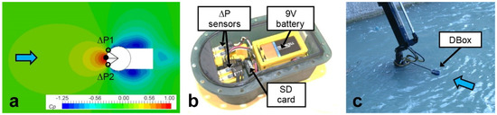
Figure 6.
(a) Computational fluid dynamics (CFD) simulation results showing the spatial distribution of the pressure coefficient, Cp, for a freestream velocity of 50 cm/s. The solid circle corresponds to the stagnation point, and the open circles the two differential ports ΔP1 and ΔP2. (b) Photograph of the device including the two differential pressure sensors, as well as the 9V power supply and SD data storage card. (c) Image of the DBox in the field at the HPP Kirchbichl, mounted on the large debris removal arm. Water flow direction shown as a blue arrow.
This approach to assess the local flow turbulence follows the use of Kpv in a comprehensive study on the 3D hydrodynamics of a trash rack, with different bar element angles to assess the turbulence in the local flow [50]. Here we adopt the same formulation to assess the relationship between the differential pressure fluctuations and time-averaged velocities, which were obtained using the DBox at selected measuring points. Measurements were recorded at 5 m intervals across the channel and at three depth ranges (0.5–1, 1.5–2.0 and 2.0–2.5 m). Afterwards, the measurements were compared to the spatial map of the velocity field measured by the ADCP.
Measurements were taken at each location by mounting the DBox on the large debris removal arm (Figure 6c). To mitigate external effects of measurement system on the sensor body, it was mounted on a 1 m long rectangular steel pipe, and the large mass of the arm relative to the upstream flow was found to effectively dampen against oscillations of the mounting system. Bulk velocity estimates (n = 24, range: 0.3–1.2 m/s) used in Equation (2) were calibrated using a linear regression fit (R² = 0.73) based on the time-averaged data obtained from an acoustic Doppler current profiler (ADCP Workhorse 1200 kHz; RDI Teledyne). The software WinRiver II (Teledyne Marine, Poway, USA) and Agila 7.6 (Bundesanstalt für Gewässerkunde, Koblenz, Germany) was used for processing the ADCP data. Once calibrated using field data, the high-speed (50 Hz) velocity fluctuations from the DBox provide a flow turbulence distribution, which is not possible when using a moving ADCP [51]. The probe thus provides a new source of spatially distributed flow turbulence data. When combined with the ADCP time-averaged velocity field and fish spatial preferences, it becomes possible to study a wider range of hydrodynamic stimuli, which fish experience upstream of trash racks. Spatially resolved data is needed in order to understand the underlying mechanisms, which control fish migration in terms of the timing, direction and distances associated with underwater stimuli [52].
3. Results
3.1. Long-Term Assessment Based on EK15 Echosounders
The long-term data acquisition and fish detection tests were carried out from February 2015 to March 2016. Based on long-term monitoring, it was observed that the majority of fish were detected in the spring [23]. It should be noted that difficulties arose during the summer (false positive detections), caused by noise related to higher discharges as well as grass cutting. Noise was also problematic in autumn due to falling and entrained leaves, as well as in winter, caused by floating snow from urban snow clearance activities.
A sample of the long-term dataset is presented for April 2015 (Figure 7), taking into account the abiotic parameters from the river gauging station at Rattenberg. The number of detected fish-echoes (contacts) resulted in between 2 and 23 tracks per day, with multiple detections being likely.
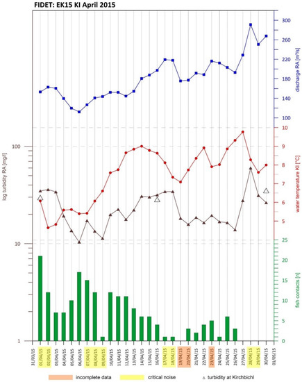
Figure 7.
EK15 fish contacts summary compared with the abiotic parameters of water temperature, runoff and turbidity during April 2015. Discharge and turbidity are from gauging station Rattenberg (about 20 km upstream), while water temperature was measured in the headrace channel of the HPP Kirchbichl. Additional measurements of turbidity at Kirchbichl show, that the data from the upstream gauging station is representative.
3.2. Investigation of Fish Behavior
Acoustic cameras were used for observations of individual fish, providing information on the spatial distribution of fish. In the depth horizons (DIDSON 1 and 2) a total of 871 fish contacts (from 9 h sonar data ≙ 97 fish contacts h−1), with n = 192 on the orographic right (i.e., true right-hand bank, looking downstream) and n = 679 on the orographic left bank were registered within the survey in spring 2017 (e.g. Video S2). Most detections (Σ 376 ≙ 125 fish contacts h−1) took place in the 1 m horizon, with 110 detections right and 266 on the left side. The cumulative contact numbers on the left are significantly higher in all horizons than on the right. In the 2 m horizon 46 detections were registered on the right and 164 on the left (Σ 210 ≙ 70 fish contacts h−1). The largest difference in contacts between the right (n = 36) and left bank (n = 249) was observed in the 3 m horizon (Σ 285 ≙ 95 fish contacts h−1).
The evaluation of continuous data from the 3 m horizon revealed 6776 fish contacts (897 on the right and 5879 on the left bank). Thus, in both DIDSON setups (horizons + continuous) 7647 fish contacts (n = 1089 right and n = 6558 left) were recorded. Regarding their length distribution, there is a clear peak of the length classes 20–30 cm and 30–40 cm. Taking into account the significantly different contact numbers, there were no significant differences for the length of frequencies on the right and left (Figure 8). This also applies to the comparison of the contact numbers in the day and night aspect, with more fish contacts being registered on the left bank in the night aspect than during the day (Figure 8). No-cross-talk was observed for the two DIDSONs running in parallel. The signal to noise ratio provided high quality data at 1.8 MHz but resolution was too poor at 1.1 MHz. However, cross-talk would have been likely for the lower frequency.
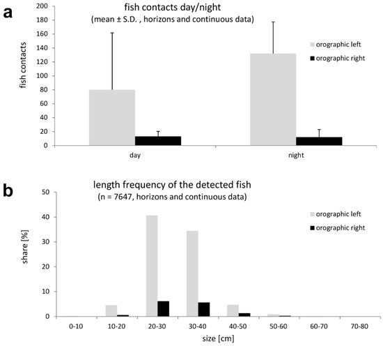
Figure 8.
(a) Day versus night comparison (in early April sunrise = 06:45, sunset = 19:50; according to www.zamg.at) of the number of fish contacts h−1 and (b) the length frequency of the detected fish (based on the evaluated data sets of 49 h sonar data from the period 4–8 April 2017).
Considering the vertical data acquisition (ARIS, Figure 9a) over six positions along the trash rack, a total of 343 fish contacts (≙114 fish contacts h−1) were registered up to a water depth of 9 m (e.g. Video S3). Considering all depth intervals, position 1 accounted for about one third of all contacts (n = 117), while towards the right bank the contacts continuously decreased (Figure 9b). Within position 1 more than two-thirds of the contacts (n = 81) were found at depths between 4 and 8 m.
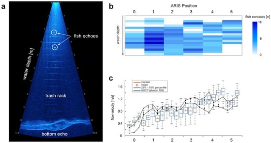
Figure 9.
(a) Two fish echoes at the trash rack (video frame from the ARISFish software). (b) Cumulative plot of fish contacts (in depth steps of 0.5 m water column) in front of the trash rack (based on 3 h of vertically recorded sonar data in the period 05–07 April 2017) and (c) Plot of ADCP (black lines form lower and upper bounds) and DBox calibration data as box plots.
3.3. Flow Turbulence
The evaluation of the ADCP data shows that under the design flow of 250 m3/s, the highest flow velocities were found in the right half of the trash rack entrance (Figure 9c). The lower flow velocities and sweeping currents on the left bank are caused by the entrance geometry, as the trash rack begins with a short, 10 m horizontal offset from the left bank (Figure 5c).
The simple regression relation, Kpv = −162.1 ∗ V + 241.9 (n = 48, R2 = 0.73), between the time-averaged velocity and differential pressure turbulence was used to generate cross-sectional plots based on the ADCP data. Specifically, our interest was the interrogation of local regions within the flow field, which exhibited combinations of velocity and turbulence found in slower flowing areas that could indicate the presence of large coherent eddies (Figure 10).
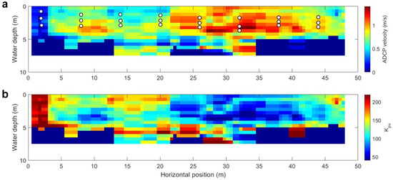
Figure 10.
Cross-section plots of the bulk velocity (in profile 189) measured by the ADCP, the locations of the 24 DBox measurements are shown as white circles with a black border (a). The plot of the pressure turbulence by combining the differential pressure fluctuations and bulk velocity measurements following Equation (2) (b). Note the linear relationship between the bulk velocity and turbulence (dynamic pressure coefficient). Thus, the spatial distribution of the intensities was found to be inversely proportional for this case study. At Kirchbichl, regions with high Kpv had on average, lower flow velocities.
4. Discussion
It is not feasible to simultaneously monitor fish presence and behavior in a large alpine river using conventional methodologies, such as netting (german “Hamen” [53]). Therefore, the FIDET project developed a multimodal sensing approach by combining hydroacoustic observations of fish with hydrodynamic variables by measuring the time-averaged velocity and pressure turbulence.
Single-beam echosounders have been successfully applied to assess and monitor fish presence at several hydroelectric sites [54,55,56]. We used a comparable setup in a large alpine river, which provided the first long-term dataset of this river type. In terms of practicality, it was found that the echosounder installation has the potential to detect fish under the wide range of natural conditions demanded for in situ investigations. However, it should be noted that an unfavorable ratio of signal strength to background noise can severely limit detection [57]. In addition, it is necessary to devise a deployment strategy, which allows for the quick removal of the echosounders during discharges with high debris loadings or during flood events. Therefore, it is highly recommended that the experimental plan explicitly includes a maintenance design and hands-on training for responsible personnel, as periodic cleaning and removal of the floats is a key factor enabling long-term measurements. Furthermore, the device positioning should be determined on a case-by-case decision. However, in an alpine river with strong flood events and related floating debris (wood, sediment) the proposed setup (floats that can be recovered) is the only feasible one. An upward-looking array would require installation, inspection, and safe removal by divers prior to floods. This was considered impractical at this site.
The development of site-specific tracking criteria was found to provide a useful basis for future studies under similar conditions. For example, the variability in TS values in the field trials was expected to be large, as it is a single-beam system with large opening angles. The detection of an object’s orientation and absolute size determination is thus at best only partially feasible. While the detection was satisfactory in spring and early summer, problems did occur due to (1) noise caused by high discharges, (2) organic material (e.g., grass clippings, leaves, wood) and (3) snow and ice related to dumping of snow into rivers. In general, the echosounder-based fish tracking system provided a cost-effective long-term monitoring system, however the mentioned limitations need to be considered.
In order to assess fish behavior, a multimodal hydroacoustic and pressure measurement system was developed and implemented for the first time, taking into accounts the parallel use of three imaging sonars. The data collected present new insights using non-invasive measurement technologies on fish presence and behavior in front of a large, run-of-river hydropower intake. Specifically, the combination of spatially distributed, time-averaged flow velocities recovered from the ADCP and pressure turbulence measurements form the dynamic picture of the complex flow field experienced by fish in front of hydropower intakes. While acoustic cameras are capable of capturing underwater videos, which enable investigations of fish behavior, a long-term deployment “in the field” is limited due to equipment as well as operational costs. During the deployment of the DIDSON and ARIS systems, personnel had to be present on site in order to avoid damage caused by floating debris and to adapt the setup due to operational requirements (e.g., different depth horizons). Also, the manual post-processing is time-consuming; i.e., a factor of 1:3 between field work and post-processing has to be considered. We used the sonar data for individual fish observation, but the data could also support the analyses of swimming paths of individual fish [58]. However, acoustic cameras could either be used in a certain case study (as presented herein) or possibly be installed at a safe-site for long term monitoring (e.g., within a chamber of a by-pass system).
There are limitations due to orientation and range, but acoustic cameras have a high potential for underwater investigations, including technical inspections as well as biological surveys. Acoustic cameras have been sporadically used to detect and investigate fish and their behavior in close vicinity of hydroelectric sites in recent years [39,59]. ARIS was used by Mendez et al. [60] to investigate activity of adult lake trout in the headrace channel of a hydropower plant in Switzerland. In this regard, our setup of an acoustic camera triplet in front of an alpine run-off river power plant is a novel application to assess the temporal and distribution pattern of fish.
The majority of fish contacts were found to occur in the border area (ARIS position 1; Figure 9b) between turbulent and recirculating flow. Thus, our data suggest that different flow fields in the border area between turbulent and recirculating flow are preferred by fish. Considering the evaluation of the data from the horizontal setup this difference is significant and formed the basis for detailed design of a bypass. Confirmed by visual contacts and expert opinion, the majority of the fish are rainbow trout. The spatial analysis of the fish contact numbers (taking into accounts the sonar locations, alignments, ranges, and water depths) with the flow field, indicate that the majority of fish contacts was made at the interface between turbulent and calm water on the orographic left side. This is an important key for the design of a sustainable mitigation measure, in order to guide the fish into a bypass system. Further, it was shown that the use of a new differential pressure-based field turbulence measurement device can be correlated to ADCP measurements of the time-averaged flow field, revealing turbulent flow regions that may guide or repel fish. These regions could be more attractive to larger fish because studies on trout swimming in such eddies have shown that fish can use such eddies to reduce their energy consumption [61]. Based on this hypothesis, it could be the case that adult fish are observed on the leftmost 10 m of the hydropower intake and are less likely to be present in high-velocity regions with an overall lower turbulence parameter (Figure 10b). These patterns were confirmed by the analyses using DIDSON sonar or ARIS (Figure 9c), indicating the potential of the proposed turbulence parameter for predicting fish behavior in front of hydropower intakes.
The combined time-averaged velocity and pressure turbulence measurements were chosen based on literature studies of fish sensory capabilities, where it has been experimentally determined that fish respond to bulk fluid forcing in conjunction with local fluctuations in the pressure field [62]. Within a turbulent flow field, fish experience these fluctuations at a rate directly proportional to the local flow speed, and thus the ratio of the fluctuations to the local flow speed may prove to be a useful indictor of fish behavior considering in situ flow environments [63]. Further studies should compare the distribution of flow turbulence using the proposed methodology with additional field observations to determine hydraulic preferences relevant to fish.
It is also important to consider plant-specific characteristics including the turbine type and discharge conditions. At the HPP Kirchbichl, there currently exist downstream migration pathways via the weir during overflow, via the open weir during flood events, or by turbine passage (Kaplan turbine). After the ongoing expansion of HPP Kirchbichl there will be additional migration pathways: (1) Through a newly constructed fishway, (2) through a new bypass at the weir and (3) a new bypass at the end of the headrace canal. Within the extension of the HPP among other measures, the headrace channel in front of the HPP will extend beyond the left bank, promoting a larger area with reduced flow velocity. In this region, a fish descent corridor (by-pass), with two entrance structures (an upper one and a lower one), is being built [30]. Our study suggests that fish accumulate in the border area between turbulent and recirculating flow regions, which supports attraction. Additionally, underwater lighting (at the entrance structures) will be used to guide the fish into the by-pass system. The attraction by light is known from various studies (e.g., [64]) and was recently successfully implemented to guide fish into a fish sluice [65]. The planned monitoring at the HPP Kirchbichl after the implementation of these measures will provide a further contribution to knowledge about fish descent routes under real conditions.
5. Conclusions
Overall, further field testing of the proposed methodology should be carried out at additional large hydropower sites covering additional biocoenotic regions. This should include multi-species environments as well as locations with dense fish assemblages (i.e., shoals). The latter aspect can be especially important for the identification of the young-of-the-year downstream drift in lowland rivers. A critical improvement for cross-comparing field sonar studies in rivers is the standardization of sonar output metrics (e.g., contacts h−1 per sampling volume; both for day-time as well as night). This is crucial, as a wider range of study sites are needed to be able to evaluate the relevance and possible scenarios for downstream fish passage. Our future goal is to develop an automated system for detection of fish in front of hydropower plants. This could support the operation of bypass systems on demand, in near real-time. For imaging sonars DIDSON and ARIS, early development steps have been carried out recently [66]: Although data processing remains a challenge in the face of large raw data file sizes generated by imaging sonars, image analysis tools can be used to simplify the required input data, and rapidly classify categories of like eel-shaped targets, single fishes, shoals, and debris.
Supplementary Materials
The following are available online at http://www.mdpi.com/2076-3417/8/10/1723/s1, Table S1: Overview on the sonar data (174 h) from the spring 2017 survey with the acoustic cameras; Video S2: Video sequence (DIDSON 300 with 1.8 MHz) at the continuous recording mode, view towards the trash rack (horizon 3, right bank); Video S3: Video sequence (ARIS 3000 with 1.8 MHz) at a vertical position, view across the trash rack towards the bottom.
Author Contributions
Conceptualization, M.B.S. and M.S.; Data curation, M.B.S.; Investigation, M.B.S., J.A.T. and M.S.; Methodology, M.B.S., J.A.T. and M.S.; Project administration, M.S.; Resources, M.B.S.; Visualization, M.S.; Writing–original draft, M.B.S., J.A.T. and M.S.
Funding
The FIDET project is initiated and funded by TIWAG (WK 196-0075, WK 196-0076). Jeffrey A. Tuhtan’s contribution was financed by the Estonian base financing grant No B53, “Octavo” and PUT grant 1690, “Bioinspired flow sensing” and IUT33-9 “Bio-inspired underwater robots”.
Acknowledgments
Thanks to Manuel Langkau and Marc Zeyer (hydroacoustic setup), Juan Francisco Fuentes-Pérez (assembly and lab testing of the DBox), Martin Linser and Matthias Völker (operation of the ADCP) as well as Wolfgang Würtenberger. We acknowledge also all helping hands on site, Othmar Obrist, Jochen Wittner, Peter Hladik as well as Jürgen Hintner and his team, all of them enabled the success of the fieldwork.
Conflicts of Interest
The authors declare no conflict of interest.
References
- Larinier, M. Upstream and downstream fish passage experience in France. In Fish Migration and Fish Bypasses, 1st ed.; Jungwirth, M., Schmutz, S., Weiss, S., Eds.; Blackwell Science Ltd.: Oxford, Country, 1998; pp. 127–145. ISBN 0-85238-253-7. [Google Scholar]
- Pavlov, D.; Lupandin, A.; Kostin, V. Downstream Migration of Fish through Dams of Hydroelectric Power Plants, 1st ed.; Nauka: Moscow, Russia, 1999; 249p. [Google Scholar]
- Larinier, M.; Travade, F. Downstream migration: Problems and facilities. Bull. Fr. Peche Piscic. 2002, 364, 181–207. [Google Scholar] [CrossRef]
- Pavlov, D.S.; Mikheev, V.N.; Lupandin, A.I.; Skorobogatov, M.A. Ecological and behavioural influences on juvenile fish migrations in regulated rivers: A review of experimental and field studies. Hydrobiologia 2008, 609, 125–138. [Google Scholar] [CrossRef]
- Munlv Nrw. Handbuch Querbauwerke, 1st ed.; Ministerium für Umwelt und Naturschutz, Landwirtschaft und Verbraucherschutz des Landes Nordrhein-Westfalen: Düsseldorf, Germany, 2005; 212p, ISBN 3-9810063-2-1. [Google Scholar]
- DWA. Fischschutz- und Fischabstiegsanlagen—Bemessung, Gestaltung, Funktionskontrolle, 2nd ed.; DWA—Deutsche Vereinigung für Wasserwirtschaft, Abwasser und Abfall e.V.: Hennef, Germany, 2005; 356p. [Google Scholar]
- Forum Fischschutz. Available online: https://forum-fischschutz.de (accessed on 11 March 2018).
- Nunn, A.D.; Cowx, I.G. Restoring River Connectivity: Prioritizing Passage Improvements for Diadromous Fishes and Lampreys. Ambio 2012, 41, 402–409. [Google Scholar] [CrossRef] [PubMed]
- Nyqvist, D.; Bergman, E.; Calles, O.; Greenberg, L. Intake Approach and Dam Passage by Downstream-migrating Atlantic Salmon Kelts. River Res. Appl. 2017, 33, 697–706. [Google Scholar] [CrossRef]
- Stein, F.; Doering-Arjes, P.; Fladung, E.; Brämick, U.; Bendall, B.; Schröder, B. Downstream Migration of the European Eel (Anguilla anguilla) in the Elbe River, Germany: Movement Patterns and the Potential Impact of Environmental Factors. River Res. Appl. 2016, 32, 666–676. [Google Scholar] [CrossRef]
- Verhelst, P.; Buysse, D.; Reubens, J.; Pauwels, I.; Aelterman, B.; Van Hoey, S.; Goethals, P.; Coeck, J.; Moens, T.; Mouton, A. Downstream migration of European eel (Anguilla anguilla L.) in an anthropogenically regulated freshwater system: Implications for management. Fish. Res. 2018, 199, 252–262. [Google Scholar] [CrossRef]
- Larinier, M. Fish Passage Experience at Small-Scale Hydro-Electric Power Plants in France. Hydrobiologia 2008, 609, 97–108. [Google Scholar] [CrossRef]
- Økland, F.; Teichert, M.A.K.; Thorstad, E.B.; Havn, T.B.; Heermann, L.; Sæther, S.A.; Diserud, O.H.; Tambets, M.; Hedger, R.D.; Borcherding, J. Downstream Migration of Atlantic Salmon Smolt at Three German Hydropower Stations; NINA Report 1203; NINA Publications: Bonn, Germany, 2016; pp. 1–47. ISBN 978-82-426-2832-9. [Google Scholar]
- Ulrich, J.; Mendez, R.; Kriewitz, C.R. Lösungen für den Fischabstieg am Columbia River (USA). Wasser Energie Luft 2015, 3, 187–192. [Google Scholar]
- Schmidt, M.; Schletterer, M. Hydroakustische Detektion und Fischverhalten an einer großen Wasserkraftanlage: Beispiel Tiroler Inn (Kirchbichl). WasserWirtschaft 2017, 2–3, 65–70. [Google Scholar] [CrossRef]
- Reckendorfer, W.; Loy, G.; Ulrich, J.; Heiserer, T.; Carmignola, G.; Kraus, C.; Zemanek, F.; Schletterer, M. Maßnahmen zum Schutz der Fischpopulation-die Sicht der Betreiber großer Wasserkraftanlagen. WasserWirtschaft 2017, 2–3, 82–86. [Google Scholar] [CrossRef]
- BMLFUW. Nationaler Gewässerbewirtschaftungsplan 2015; BMLFUW: Wien, Austria, 2017; 358p. [Google Scholar]
- Böttcher, H.; Unfer, G.; Zeiringer, B.; Schmutz, S.; Aufleger, M. Fischschutz und Fischabstie-Kenntnisstand und aktuelle Forschungsprojekte in Österreich. Österreichische Wasser Abfallwirtschaft 2015, 67, 299–306. [Google Scholar] [CrossRef]
- Schneider, J.; Ratschan, C.; Heisey, P.; Avalos, C.; Tuhtan, J.; Haas, C.; Reckendorfer, W.; Schletterer, M.; Zitek, A. Flussabwärts gerichtete Fischwanderung an mittelgroßen Fließgewässern in Österreich. WasserWirtschaft 2017, 12, 33–38. [Google Scholar] [CrossRef]
- Godlewska, M.; Świerzowski, A.; Winfield, I. Hydroacoustics as a tool for studies of fish and their habitat. Ecohydrol. Hydrobiol. 2004, 4, 417–427. [Google Scholar]
- Hoffmann, A.; Schmidt, M.; Lehmhaus, B.; Langkau, M.; Kühlmann, M.; Jesse, M.; Klinger, H.; Belting, K.; Weimer, P. Fischschutzmöglichkeiten an Wasserkraftanlagen. Nat. NRW 2010, 4, 21–25. [Google Scholar]
- Adam, B.; Lehmann, B. Ethohydraulik: Grundlagen, Methoden und Erkenntnisse, 1st ed.; Springer: Heidelberg, Germany; Dortrecht, The Netherlands; London, UK; New York, NY, USA, 2011; p. 351. ISBN 978-3-642-17210-6. [Google Scholar]
- Schmidt, M.; Langkau, M.; Zeyer, M.; Schletterer, M. Fischdetektion an Rechen großer Wasserkraftanlagen mittels akustischer Kameras. WasserWirtschaft 2017, 12, 39–44. [Google Scholar] [CrossRef]
- Coutant, C.C.; Whitney, R.R. Fish behavior in relation to passage through hydropower turbines: A review. Trans. Am. Fish. Soc. 2000, 129, 351–380. [Google Scholar] [CrossRef]
- Tritico, H.M.; Cotel, A.J. The effects of turbulent eddies on the stability and critical swimming speed of creek chub (Semotilus atromaculatus). J. Exp. Biol. 2010, 213, 2284–2293. [Google Scholar] [CrossRef] [PubMed]
- Smith, D.L.; Goodwin, R.A.; Nestler, J.M. Relating Turbulence and Fish Habitat: A New Approach for Management and Research. Rev. Fish. Sci. Aquac. 2014, 22, 123–130. [Google Scholar] [CrossRef]
- Langford, M.T.; Robertson, C.B.; Zhu, D.Z.; Leake, A. Evaluation of the Viability of an Acoustic Doppler Current Profiler for the Velocity Field Analysis of Fish Entrainment Risk at Hydropower Dams. In World Environmental and Water Resources Congress 2011; American Society of Civil Engineers: Reston, VA, USA, 2011; Available online: http://ascelibrary.org/doi/abs/10.1061/41173%28414%29420 (accessed on 24 June 2016).
- Bundesministerium für Verkehr und verstaatlichte Betriebe. Innkraftwerk Kirchbichl. (Österreichische Kraftwerke in Einzeldarstellungen); Verstaatlichte Betriebe, Wien, 1953 (17, p. 20 + 7 Planbeilagen); Bundesministerium f. Verkehr u.
- Gassner, H.; Jagsch, A. Hydroakustische Fischbestandserhebung der Innstaue Langkampfen und Kirchbichl. Unpublished Report KE 196-0002. 2012. [Google Scholar]
- Stockinger, W.; Spindler, T.; Wenzl, P.; Römer, J.; Hörl, C. Kraftwerk Kirchbichl—Erweiterung: Fachbeitrag Gewässerökologie; EIA Report on Aquatic Ecology and Fisheries, (KE920-0001b); TIWAG: Innsbruck, Austria, 2013. [Google Scholar]
- Kongsberg Maritime AS. Simrad EK15 Multi Purpose Scientific Echo Sounder. Available online: https://www.simrad.com/ek15 (accessed on 11 March 2018).
- LFV Hydroakustik GmbH. Fischschutz Forggensee: Hydroakustische Detektion der Fischverteilung und des Fischverhaltens am Entnahmebauwerk (OW). Unpublished report on behalf of E.ON Kraftwerke GmbH. 2015. [Google Scholar]
- Grote, A.B.; Bailey, M.M.; Zydlewski, J.D.; Hightower, J.E. Multibeam sonar (DIDSON) assessment of American shad (Alosa sapidissima) approaching a hydroelectric dam. Can. J. Fish. Aquat. Sci. 2014, 71, 545–558. [Google Scholar] [CrossRef]
- O’Connell, C.P.; Hyun, S.-Y.; Rillahan, C.B.; He, P. Bull shark (Carcharhinus leucas) exclusion properties of the sharksafe barrier and behavioral validation using the ARIS technology. Glob. Ecol. Conserv. 2014, 2, 300–314. [Google Scholar] [CrossRef]
- Martignac, F.; Daroux, A.; Bagliniere, J.-L.; Ombredane, D.; Guillard, J. The use of acoustic cameras in shallow waters: New hydroacoustic tools for monitoring migratory fish population. A review of DIDSON technology. Fish. Fish. 2015, 16, 486–510. [Google Scholar] [CrossRef]
- Handegard, N.O.; Williams, K. Automated tracking of fish in trawls using the Didson (Dual-frequency Identification Sonar). ICES J. Mar. Sci. 2008, 65, 636–644. [Google Scholar] [CrossRef]
- Hateley, J.; Gregory, J. Evaluation of a Multi-Beam Imaging Sonar System (DIDSON) as FISHERIES Monitoring Tool: Exploiting the Acoustic Advantage; Technical Report; Environment Agency: London, UK, 2008. [Google Scholar]
- Mueller, A.M.; Mulligan, T.; Withler, P.K. Classifying Sonar Images: Can a Computer-Driven Process Identify Eels? North. Am. J. Fish. Manag. 2008, 28, 1876–1886. [Google Scholar] [CrossRef]
- Adams, N.S.; Smith, C.; Plumb, J.M.; Hansen, G.S.; Beeman, J.W. An Evaluation of Fish Behavior Upstream of the Water Temperature Control Tower at Cougar Dam, Oregon, Using Acoustic Cameras; US Geological Survey, Western Fisheries Research Center: Seattle, WA, USA, 2013. [Google Scholar]
- Langkau, M.C.; Clavé, D.; Schmidt, M.B.; Borcherding, J. Spawning behaviour of Allis shad Alosa alosa: New insights based on imaging sonar data. J. Fish. Biol. 2016, 88, 2263–2274. [Google Scholar] [CrossRef] [PubMed]
- Shahrestani, S.; Bi, H.; Lyubchicha, V.; Boswell, K.M. Detecting a nearshore fish parade using the adaptive resolution imaging sonar (ARIS): An automated procedure for data analysis. Fish. Res. 2017, 191, 190–199. [Google Scholar] [CrossRef]
- Belcher, E.O.; Matsuyama, B.; Trimble, R. Object identification with acoustic lenses. In Proceedings of the Conference MTS/IEEE Oceans, Honolulu, HI, USA, 5–8 November 2001; Volume 1, pp. 6–11. [Google Scholar]
- Burwen, D.L.; Fleischman, S.J.; Miller, J.D. Accuracy and precision of salmon length estimates taken from DIDSON sonar images. Trans. Am. Fish. Soc. 2010, 139, 1306–1314. [Google Scholar] [CrossRef]
- Tušer, M.; Frouzová, J.; Balk, H.; Muška, M.; Mrkvička, T.; Kubečka, J. Evaluation of potential bias in observing fish with a DIDSON acoustic camera. Fish. Res. 2014, 155, 114–121. [Google Scholar] [CrossRef]
- Penney, G.W.; Fechheimer, C.J. Abridgment of thermal volume meter. J. AIEE 1928, 47, 181–184. [Google Scholar] [CrossRef]
- Fuentes-Pérez, J.F.; Meurer, C.; Tuhtan, J.A.; Kruusmaa, M. Differential Pressure Sensors for Underwater Speedometry in Variable Velocity and Acceleration Conditions. IEEE J. Ocean. Eng. 2018, 43, 418–426. [Google Scholar] [CrossRef]
- Fuentes-Pérez, J.F.; Kalev, K.; Tuhtan, J.A.; Kruusmaa, M. Underwater vehicle speedometry using differential pressure sensors: Preliminary results. In Autonomous Underwater Vehicles (AUV), 2016 IEEE/OES; IEEE: Piscataway, NJ, USA, 2016; pp. 156–160. [Google Scholar]
- Schletterer, M.; Götsch, H.; Tuhtan, J.A.; Fuentes-Perez, J.F.; Kruusmaa, M. More than depth: Developing pressure sensing systems for aquatic environments. In Proceedings of the HydroSenSoft, International Symposium and Exhibition on Hydro-Environment Sensors and Software, Madrid, Spain, 1–3 March 2017. [Google Scholar]
- Neuhart, D.H.; Jenkins, L.N.; Choudhari, M.M.; Khorrami, M.R. Measurements of the flowfield interaction between tandem cylinders. In Proceedings of the 15th AIAA/CEAS Aeroacoustics Conference 30th AIAA Aeroacoustics Conference, Miami, FL, USA, 11–13 May 2009; p. 3275. [Google Scholar]
- Zhang, Y.O.; Zhang, T.; Ouyang, H.; Li, T.Y. Flow-induced noise analysis for 3D trash rack based on LES/Lighthill hybrid method. Appl. Acoust. 2014, 79, 141–152. [Google Scholar] [CrossRef]
- Nystrom, E.A.; Rehmann, C.R.; Oberg, K.A. Evaluation of mean velocity and turbulence measurements with ADCPs. J. Hydraul. Eng. 2007, 133, 1310–1318. [Google Scholar] [CrossRef]
- Smith, R.J.F. The Control of Fish Migration; Springer Science & Business Media: Berlin, Germany, 1985; ISBN 978-3-642-82348-0. [Google Scholar]
- Pander, J.; Mueller, M.; Knott, J.; Geist, J. Catch-related fish injury and catch efficiency of stow-netbased fish recovery installations for fish-monitoring at hydropower plants. Fish. Manag. Ecol. 2018, 25, 31–43. [Google Scholar] [CrossRef]
- Ransom, B.H.; Steig, T.W. Using Hydroacoustics to Monitor Fish at Hydropower Dams. Lake Reserv. Manag. 1994, 9, 163–169. [Google Scholar] [CrossRef]
- Steig, T.W.; Iverson, T.K. Acoustic monitoring of salmonid density, target strength, and trajectories at two dams on the Columbia River, using a split-beam scanning system. Fish. Res. 1998, 35, 43–53. [Google Scholar] [CrossRef]
- Loures, R.C.; Pompeu, P.S. Seasonal and diel changes in fish distribution in a tropical hydropower plant tailrace: Evidence from hydroacoustic and gillnet sampling. Fish. Manag. Ecol. 2015, 22, 185–196. [Google Scholar] [CrossRef]
- Simmonds, E.J.; MacLennan, D.N. Fisheries Acoustics, 2nd ed.; Blackwell Science: Oxford, UK, 2005. [Google Scholar]
- Piper, A.T.; Rosewarne, P.J.; Wright, R.M.; Kemp, P.S. The impact of an Archimedes screw hydropower turbine on fish migration in a lowland river. Ecol. Eng. 2018, 118, 31–42. [Google Scholar] [CrossRef]
- Langkau, M.C. Echoes in motion: An acoustic camera (DIDSON) as a monitoring tool in applied freshwater ecology. Ph.D. Thesis, University of Cologne, Cologne, Germany, 2017; p. 89. [Google Scholar]
- Mendez, R.; Riesen, P.; Wyss, C. Untersuchungen zur Aktivität von Adulten Seeforellen am Oberwasserkanal und Stauwehr mit bildgebenden Sonar. Axpo Power AG (Internal report, Baden, Switzerland). 2017, p. 69. Available online: https://www.gr.ch/DE/institutionen/verwaltung/bvfd/ajf/dokumentation/Fischerei_Publikationen/KWR%20Auswertung%20ARIS%20Sonaraufnahmen%20Bericht_Final%202016.pdf (accessed on 7 April 2018).
- Klein, A.; Bleckmann, H. The muscle activity of trout exposed to unsteady flow. J. Comp. Physiol. A 2017, 203, 163–173. [Google Scholar] [CrossRef] [PubMed]
- Mufeed, O.; Noreika, J.F.; Haro, A.; Maynard, A.; Castro-Santos, T.; Cada, G.F. Evaluation of the Effects of Turbulence on the Behavior of Migratory Fish; Final Report to the Bonneville Power Administration, Contract 22; US Department of Energy: Washington, DC, USA, 2002.
- Wang, H.; Chanson, H. Modelling upstream fish passage in standard box culverts: Interplay between turbulence, fish kinematics, and energetics. River Res. Appl. 2018, 34, 244–252. [Google Scholar] [CrossRef]
- Juell, J.-E.; Fosseidengen, J.E. Use of artificial light to control swimming depth and fish density of Atlantic salmon (Salmo salar) in production cages. Aquaculture 2004, 233, 269–282. [Google Scholar] [CrossRef]
- Fischer, J.; Schmalz, M. Optimierung der Druckkammerschschleuse mit energetischer Nutzung an der Talsperre Höllenstein. WasserWirtschaft 2015, 105, 38–41. [Google Scholar] [CrossRef]
- Schmidt, M.; Hoffmann, A.; Heermann, J.; Langkau, M.; Zeyer, M. Didson-Based Object Tracking (D-BOT)—Fischdetektion in Echtzeit als Maßnahmen- und Schutzinstrument an Wasserkraftanlagen. WasserWirtschaft 2018, 9, 49–53. [Google Scholar] [CrossRef]
© 2018 by the authors. Licensee MDPI, Basel, Switzerland. This article is an open access article distributed under the terms and conditions of the Creative Commons Attribution (CC BY) license (http://creativecommons.org/licenses/by/4.0/).