
Composite Kernel Method for PolSAR Image Classification Based on Polarimetric-Spatial Information


Abstract
:1. Introduction
2. Related Work
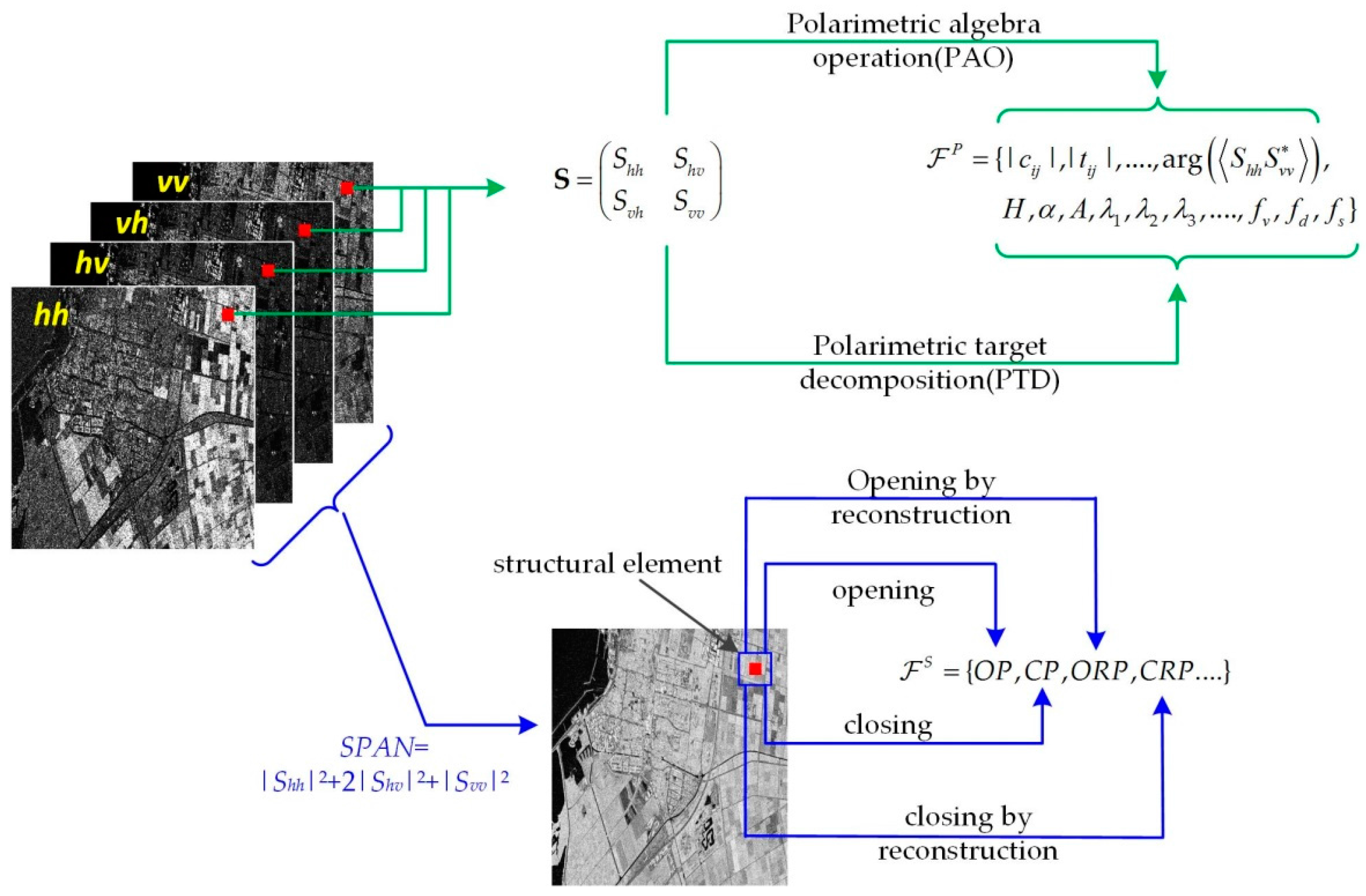
2.1. Polarimetric and Spatial Features of PolSAR Image
2.1.1. Polarimetric Features
2.1.2. Spatial Features
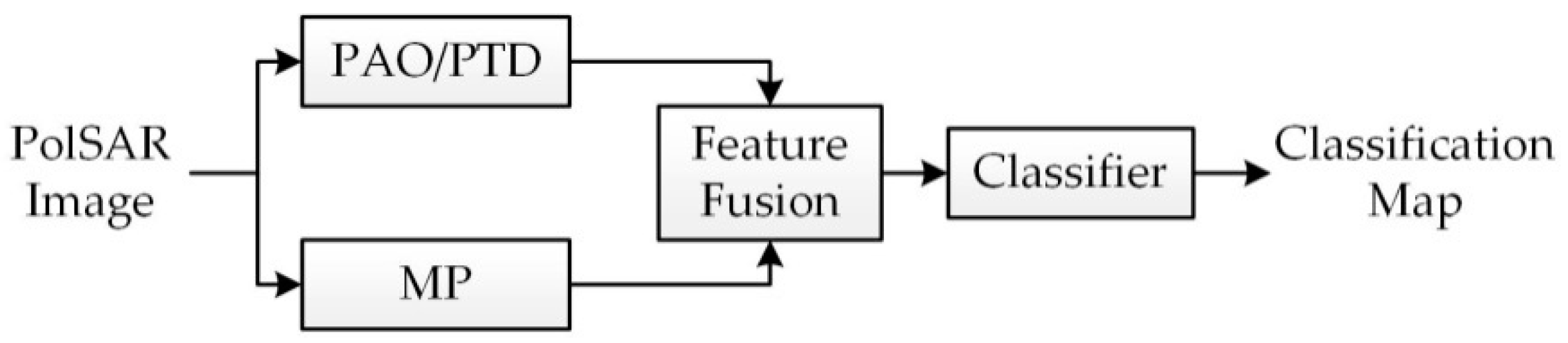
2.2. Stacked Feature Fusion
3. Composite Kernels for SVM
3.1. SVM and Kernel
3.2. Composite Kernels
- Linear kernel: .
- Polynomial kernel: .
- Radial basis function:
4. Experiment
4.1. Data Description
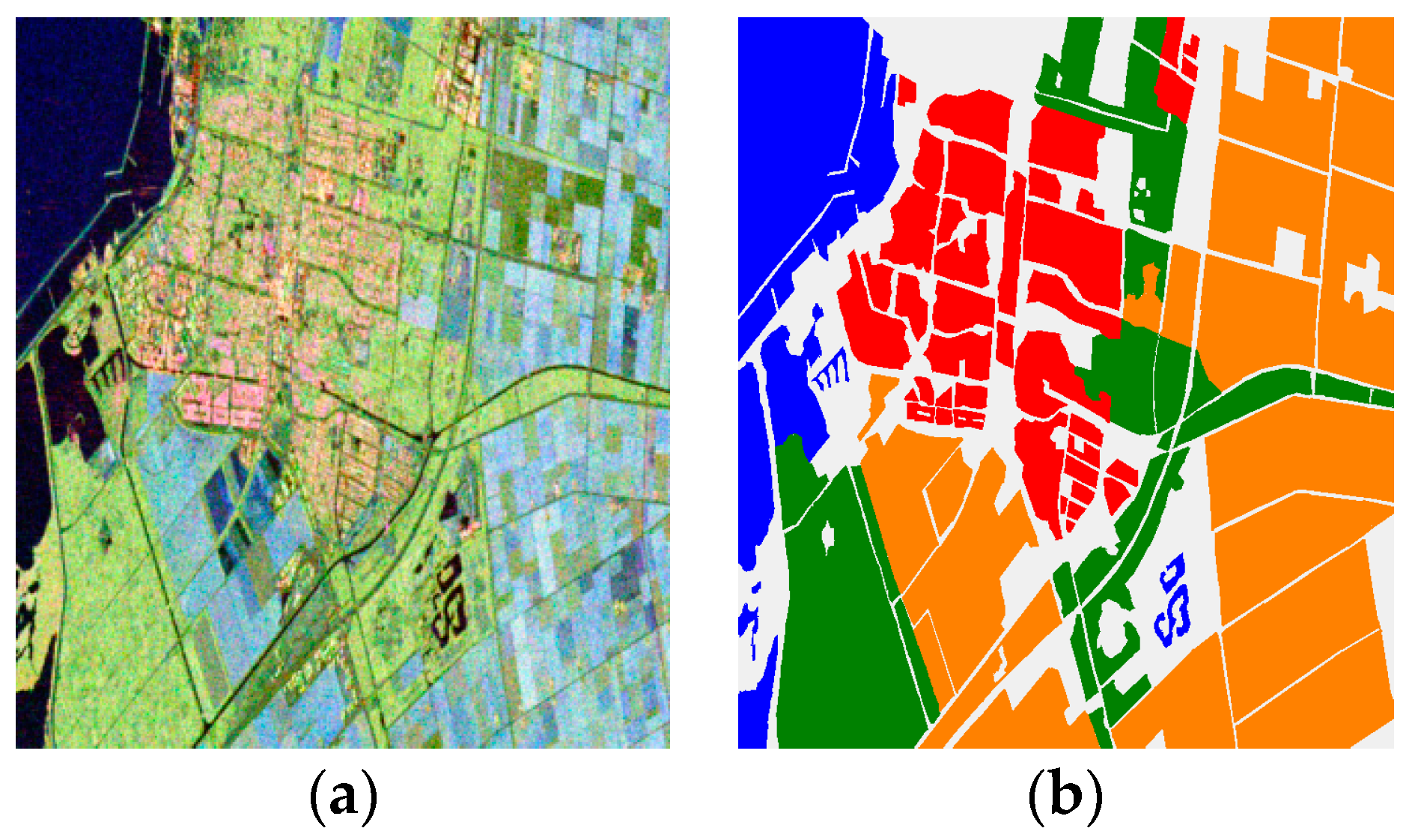
4.1.1. Flevoland Data Set
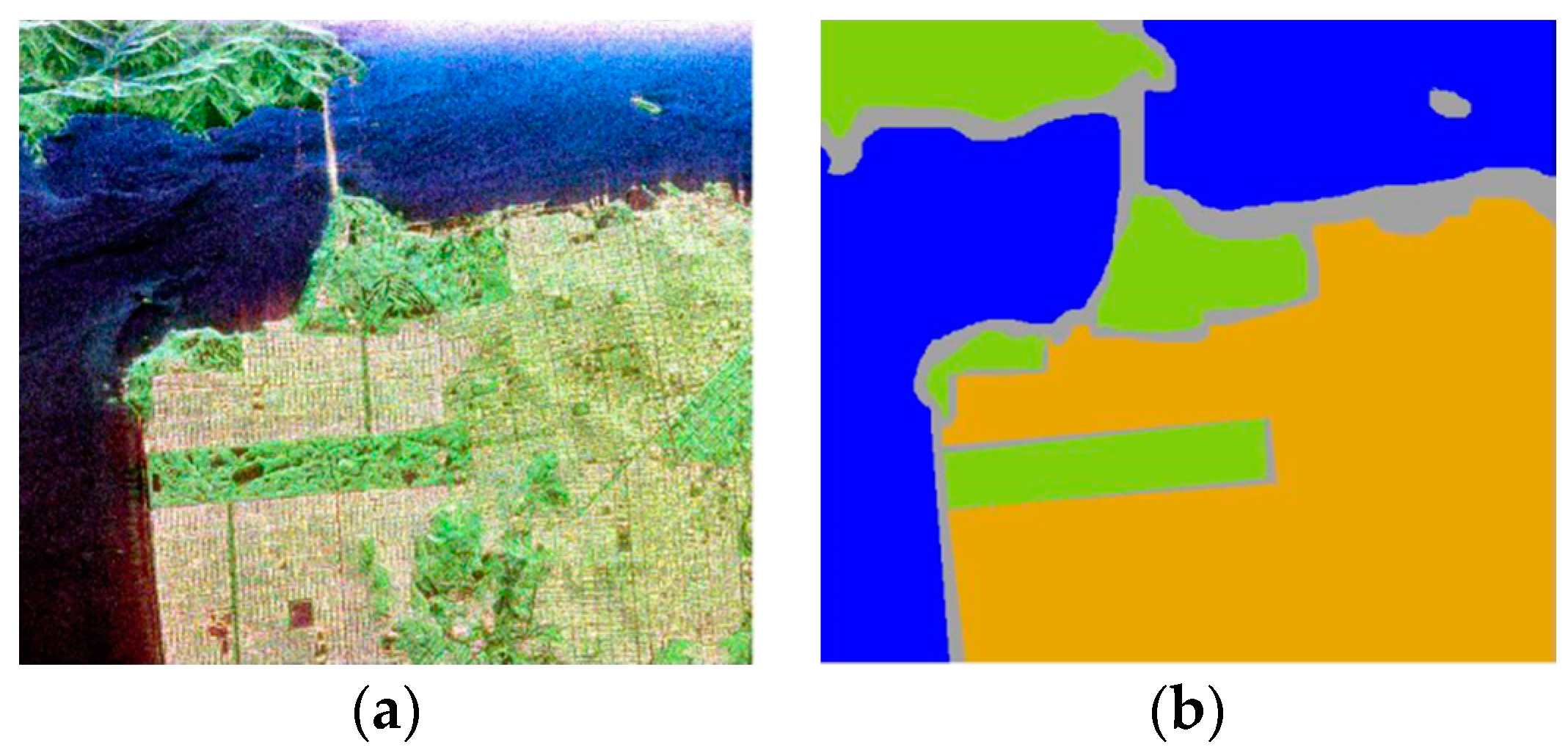
4.1.2. San Francisco Bay Data Set
4.2. General Setting
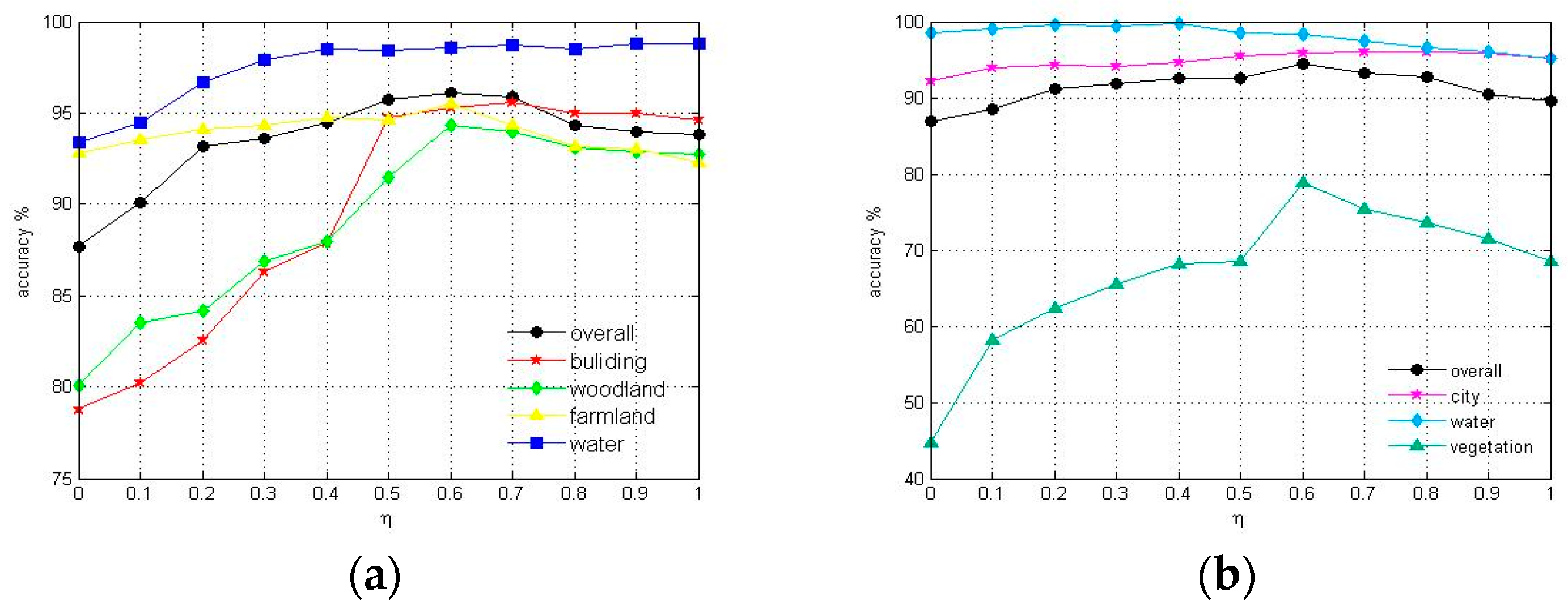
4.3. Results
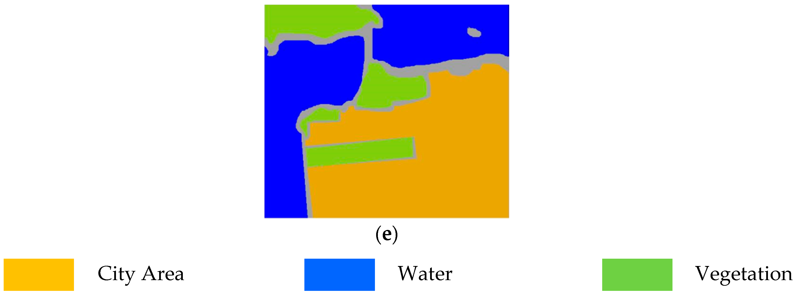
4.3.1. Flevoland Data Set
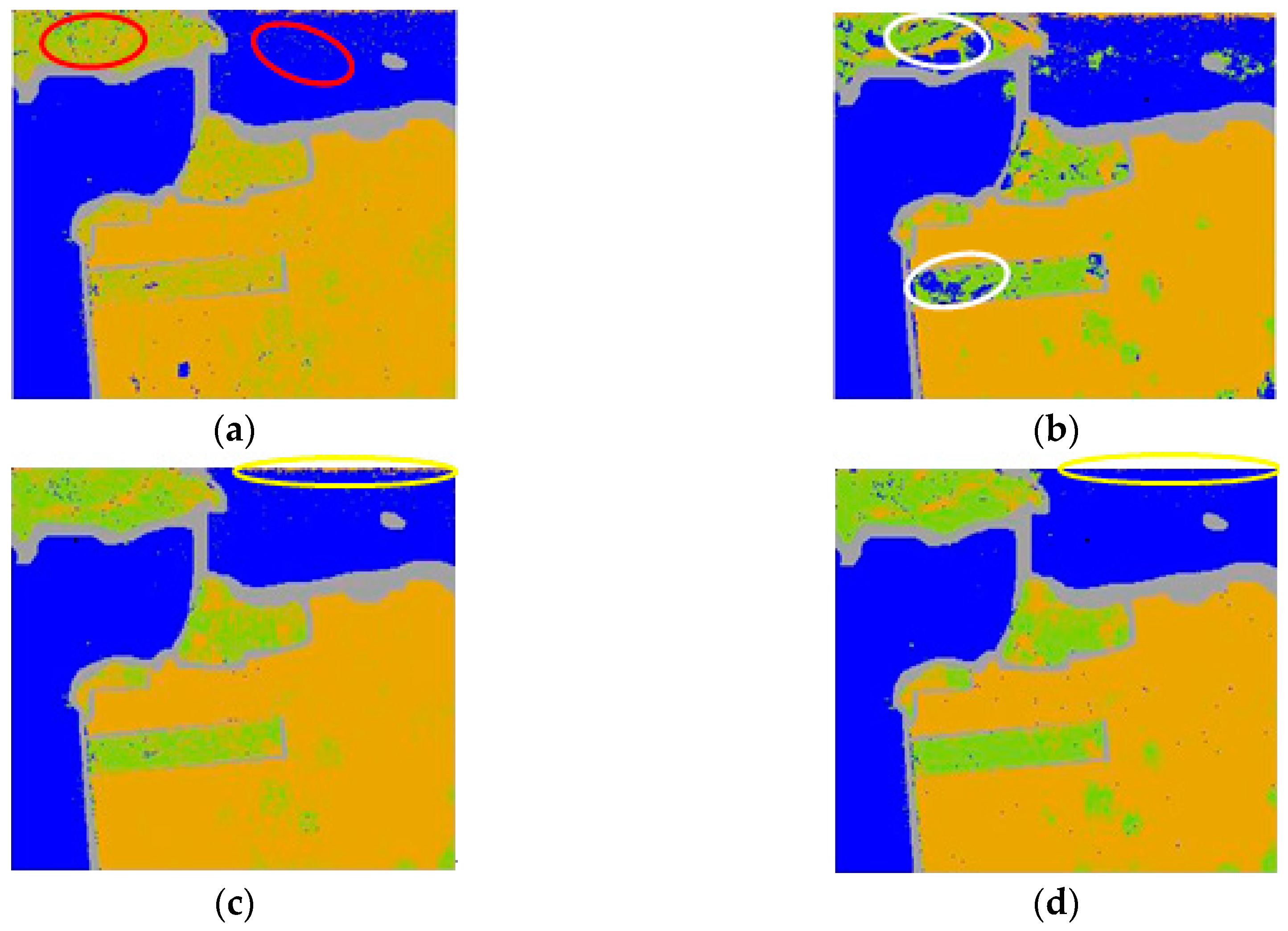
4.3.2. San Francisco Bay Data Set
5. Conclusions and Future Work
Acknowledgments
Author Contributions
Conflicts of Interest
References
- Touzi, R.; Boerner, W.M.; Lee, J.S.; Lueneburg, E. A review of polarimetry in the context of synthetic aperture radar: Concepts and information extraction. Can. J. Remote Sens. 2004, 30, 380–407. [Google Scholar] [CrossRef]
- Lee, J.-S.; Pottier, E. Polarimetric Radar Imaging: From Basics to Applications; CRC Press: Boca Raton, FL, USA, 2009. [Google Scholar]
- Doulgeris, A.P.; Anfinsen, S.N.; Eltoft, T. Automated non-Gaussian clustering of polarimetric synthetic aperture radar images. IEEE Trans. Geosci. Remote Sens. 2001, 49, 3665–3676. [Google Scholar] [CrossRef]
- Liu, H.-Y.; Wang, S.; Wang, R.-F. A framework for classification of urban areas using polarimetric SAR images integrating color features and statistical model. J. Infrared Millim. Waves 2016, 35, 398–406. [Google Scholar]
- Fan, K.T.; Chen, Y.S.; Lin, C.W. Identification of rice paddy fields from multitemporal polarimetric SAR images by scattering matrix decomposition. In Proceedings of the IEEE International Symposium on Geoscience and Remote Sensing IGARSS, Milan, Italy, 26–31 July 2015; pp. 3199–3202. [Google Scholar]
- Cloude, S.R.; Pottier, E. A review of target decomposition theorems in radar polarimetry. IEEE Trans. Geosci. Remote Sens. 1996, 34, 498–518. [Google Scholar] [CrossRef]
- Yuan, H.; Tang, Y.Y. Spectral-Spatial Shared Linear Regression for Hyperspectral Image Classification. IEEE Trans. Cybern. 2017, 47, 934–945. [Google Scholar] [CrossRef] [PubMed]
- Zou, T.; Yang, W.; Dai, D.; Sun, H. Polarimetric SAR Image Classification Using Multifeatures Combination and Extremely Randomized Clustering Forests. EURASIP J. Adv. Signal Process. 2010, 2010, 4. [Google Scholar] [CrossRef]
- Tu, S.T.; Chen, J.Y.; Yang, W.; Sun, H. Laplacian eigenmaps based polarimetric dimensionality reduction for SAR image classification. IEEE Trans. Geosci. Remote Sens. 2012, 50, 170–179. [Google Scholar] [CrossRef]
- Shi, L.; Zhang, L.; Yang, J. Supervised graph embedding for polarimetric SAR image classification. IEEE Geosci. Remote Sens. Lett. 2013, 10, 216–220. [Google Scholar] [CrossRef]
- Li, J.; Bioucas-Dias, J.M.; Plaza, A. Spectral-spatial hyperspectral image segmentation using subspace multinomial logistic regression and Markov random fields. IEEE Trans. Geosci. Remote Sens. 2012, 50, 809–823. [Google Scholar] [CrossRef]
- Moser, G.; Serpico, S.; Benediktsson, J.A. Land-cover mapping by Markov modeling of spatial–contextual information in very-high-resolution remote sensing images. Proc. IEEE 2013, 101, 631–651. [Google Scholar] [CrossRef]
- Chen, X.; Fang, T.; Huo, H.; Li, D. Graph-based feature selection for object-oriented classification in VHR airborne imagery. IEEE Trans. Geosci. Remote Sens. 2011, 49, 353–365. [Google Scholar] [CrossRef]
- Liu, B.; Hu, H.; Wang, H.; Wang, K.; Liu, X.; Yu, W. Superpixel-based classification with an adaptive number of classes for polarimetric SAR images. IEEE Trans. Geosci. Remote Sens. 2013, 51, 907–924. [Google Scholar] [CrossRef]
- Dai, D.; Yang, W.; Sun, H. Multilevel local pattern histogram for SAR image classification. IEEE Geosci. Remote Sens. Lett. 2011, 8, 225–229. [Google Scholar] [CrossRef]
- Shen, L.; Zhu, Z.; Jia, S.; Zhu, J.; Sun, Y. Discriminative Gabor feature selection for hyperspectral image classification. IEEE Geosci. Remote Sens. Lett. 2013, 10, 29–34. [Google Scholar] [CrossRef]
- Huang, X.; Zhang, L. An SVM ensemble approach combining spectral, structural, and semantic features for the classification of high-resolution remotely sensed imagery. IEEE Trans. Geosci. Remote Sens. 2013, 51, 257–272. [Google Scholar] [CrossRef]
- Soille, P. Morphological Image Analysis; Springer: Berlin, Germany, 2004. [Google Scholar]
- Devis, T.; Frederic, R.; Alexei, P.; Camps-Valls, G. Composite kernels for Urban-image classification. IEEE Geosci. Remote Sens. Lett. 2010, 7, 88–92. [Google Scholar]
- Du, P.; Samat, A.; Waskec, B.; Liu, S.; Li, Z. Random Forest and Rotation Forest for fully polarized SAR image classification using polarimetric and spatial features. ISPRS J. Photogramm. Remote Sens. 2015, 105, 38–53. [Google Scholar] [CrossRef]
- Molinier, M.; Laaksonen, J.; Rauste, Y.; Häme, T. Detecting changes in polarimetric SAR data with content-based image retrieval. In Proceedings of the IEEE International Geoscience and Remote Sensing Symposium, Barcelona, Spain, 23–28 July 2007; pp. 2390–2393. [Google Scholar]
- Krogager, E. New decomposition of the radar target scattering matrix. Electron. Lett. 1990, 26, 1525–1527. [Google Scholar] [CrossRef]
- Cloude, S.R.; Pottier, E. An entropy based classification scheme for land applications of polarimetric SAR. IEEE Trans. Geosci. Remote Sens. 1997, 35, 68–78. [Google Scholar] [CrossRef]
- Yamaguchi, Y.; Moriyama, T.; Ishido, M.; Yamada, H. Four component scattering model for polarimetric SAR image decomposition. IEEE Trans. Geosci. Remote Sens. 2005, 43, 1699–1706. [Google Scholar] [CrossRef]
- Freeman, A.; Durden, S.L. A three-component scattering model for polarimetric SAR data. IEEE Trans. Geosci. Remote Sens. 1998, 36, 963–973. [Google Scholar] [CrossRef]
- Soille, P.; Pesaresi, M. Advances in mathematical morphology applied to geoscience and remote sensing. IEEE Trans. Geosci. Remote Sens. 2002, 40, 2042–2055. [Google Scholar] [CrossRef]
- Fauvel, M.; Benediktsson, J.A.; Chanussot, J.; Sveinsson, J.R. Spectral and spatial classification of hyperspectral data using SVMs and morphological profiles. IEEE Trans. Geosci. Remote Sens. 2008, 46, 3804–3814. [Google Scholar] [CrossRef]
- Zhao, Y.-Q.; Liu, J.-X.; Liu, J. Medical image segmentation based on morphological reconstruction operation. Comput. Eng. Appl. 2007, 43, 228–240. [Google Scholar]
- Plaza, A.; Martinez, P.; Plaza, J.; Perez, R. Dimensionality reduction and classification of hyperspectral image data using sequences of extended morphological transformations. IEEE Trans. Geosci. Remote Sens. 2005, 43, 466–479. [Google Scholar] [CrossRef]
- Camps-Valls, G.; Gomez-Chova, L.; Muñoz-Mari, J.; Vila-Frances, J.; Calpe-Maravilla, J. Composite kernels for hyperspectral image classification. IEEE Geosci. Remote Sens. Lett. 2006, 3, 93–97. [Google Scholar] [CrossRef]
- Vapnik, V.N. The Nature of Statistical Learning Theory, 2nd ed.; Springer: New York, NY, USA, 2000. [Google Scholar]
- Burges, C. A tutorial on support vector machines for pattern recognition. Data Min. Knowl. Discov. 1998, 2, 121–167. [Google Scholar] [CrossRef]
- Gu, B.; Sheng, V.S. A Robust Regularization Path Algorithm for ν-Support Vector Classification. IEEE Trans. Neural Netw. Learn. Syst. 2016, 28, 1241–1248. [Google Scholar] [CrossRef] [PubMed]
- Gu, B.; Sheng, V.S.; Tay, K.Y.; Romano, W.; Li, S. Incremental Support Vector Learning for Ordinal Regression. IEEE Trans. Neural Netw. Learn. Syst. 2015, 26, 1403–1416. [Google Scholar] [CrossRef] [PubMed]
- Kim, E. Every You Wanted to Know about the Kernel Trick (But Were Too Afraid to Ask). Available online: http://www.eric-kim.net/eric-kim-net/posts/1/kernel_trick.html (accessed on 1 June 2016).
- Gu, B.; Sheng, V.S.; Wang, Z.; Ho, D.; Osman, S.; Li, S. Incremental learning for ν-Support Vector Regression. Neural Netw. 2015, 67, 140–150. [Google Scholar] [CrossRef] [PubMed]
- LIBSVM Tools. Available online: http://www.csie.ntu.edu.tw/~cjlin/libsvmtools (accessed on 1 June 2016).
- Mercer’s Theorem. Available online: https://en.wikipedia.org/wiki/Mercer%27s_theorem (accessed on 1 June 2016).
- Tuia, D.; Ratle, F.; Pozdnoukhov, A.; Camps-valls, G. Multisource composite kernels for urban-image classification. IEEE Geosci. Remote Sens. Lett. 2010, 7, 88–92. [Google Scholar] [CrossRef]
- Kappa Coefficients: A Critical Appraisal. Available online: http://john-uebersax.com/stat/kappa.htm (accessed on 1 June 2016).


| Polarimetric Signatures | Expression |
|---|---|
| Amplitude of upper triangle matrix elements of C | |
| Amplitude of upper triangle matrix elements of T | |
| Ratio between HV and HH backscattering coefficient | |
| Ratio between VV and HH backscattering coefficient | |
| Ratio between HV and VV backscattering coefficient | |
| Depolarization ratio | |
| Phase difference HH-VV | |
| Entropy, alpha angle, anisotropy and eigenvalues in Cloude Decomposition | |
| nine parameters of the Huynen Decomposition | |
| Power of surface, double-bounce, volume and helix scatter components in Yamaguchi Decomposition | |
| Coefficient for the volume, double bounce and surface components in Van Zyl Decomposition |
| Morphological Operations | Expression |
|---|---|
| Erosion | |
| Dilation | |
| Opening | |
| Closing | |
| Opening by reconstruction | |
| Closing by reconstruction |
| Class | Building | Woodland | Farmland | Water |
|---|---|---|---|---|
| Number of Samples in the Reference Map | 71,331 | 85,539 | 184,920 | 59,504 |
| Number of Training Samples | 713 | 855 | 1849 | 595 |
| Number of Testing Samples | 70,618 | 84,684 | 183,071 | 58,909 |
| Class | City Area | Water | Vegetation |
|---|---|---|---|
| Number of Samples in the Reference Map | 391,407 | 315,320 | 135,508 |
| Number of Training Samples | 3914 | 3153 | 1355 |
| Number of Testing Samples | 387,439 | 312,167 | 134,153 |
| Method | Building (%) | Woodland (%) | Farmland (%) | Water (%) | Overall Accuracy (%) | Kappa Coefficient |
|---|---|---|---|---|---|---|
| Only POL | 78.8 | 80.1 | 92.8 | 93.4 | 87.7 | 0.842 |
| Only MP | 94.6 | 92.7 | 92.3 | 98.9 | 93.8 | 0.909 |
| Vector Stacking | 95.2 | 93.7 | 96.2 | 97.4 | 95.7 | 0.920 |
| Composite Kernel | 95.6 | 94.3 | 96.2 | 98.8 | 96.1 | 0.942 |
| Method | City Area (%) | Water (%) | Vegetation (%) | Overall Accuracy (%) | Kappa Coefficient |
|---|---|---|---|---|---|
| Only POL | 92.2 | 98.5 | 44.7 | 86.9 | 0.783 |
| Only MP | 95.1 | 95.2 | 60.7 | 89.6 | 0.830 |
| Vector Stacking | 96.0 | 98.5 | 68.5 | 92.6 | 0.879 |
| Composite Kernel | 96.0 | 99.7 | 78.8 | 94.4 | 0.909 |
© 2017 by the authors. Licensee MDPI, Basel, Switzerland. This article is an open access article distributed under the terms and conditions of the Creative Commons Attribution (CC BY) license (http://creativecommons.org/licenses/by/4.0/).
Share and Cite
Wang, X.; Cao, Z.; Ding, Y.; Feng, J. Composite Kernel Method for PolSAR Image Classification Based on Polarimetric-Spatial Information. Appl. Sci. 2017, 7, 612. https://doi.org/10.3390/app7060612
Wang X, Cao Z, Ding Y, Feng J. Composite Kernel Method for PolSAR Image Classification Based on Polarimetric-Spatial Information. Applied Sciences. 2017; 7(6):612. https://doi.org/10.3390/app7060612
Chicago/Turabian StyleWang, Xianyuan, Zongjie Cao, Yao Ding, and Jilan Feng. 2017. "Composite Kernel Method for PolSAR Image Classification Based on Polarimetric-Spatial Information" Applied Sciences 7, no. 6: 612. https://doi.org/10.3390/app7060612
APA StyleWang, X., Cao, Z., Ding, Y., & Feng, J. (2017). Composite Kernel Method for PolSAR Image Classification Based on Polarimetric-Spatial Information. Applied Sciences, 7(6), 612. https://doi.org/10.3390/app7060612