Augmenting Environmental Interaction in Audio Feedback Systems ^†

Abstract

Audio feedback is defined as a positive feedback of acoustic signals where an audio input and output form a loop, and may be utilized artistically. This article presents new context-based controls over audio feedback, leading to the generation of desired sonic behaviors by enriching the influence of existing acoustic information such as room response and ambient noise. This ecological approach to audio feedback emphasizes mutual sonic interaction between signal processing and the acoustic environment. Mappings from analyses of the received signal to signal-processing parameters are designed to emphasize this specificity as an aesthetic goal. Our feedback system presents four types of mappings: approximate analyses of room reverberation to tempo-scale characteristics, ambient noise to amplitude and two different approximations of resonances to timbre. These mappings are validated computationally and evaluated experimentally in different acoustic conditions.

1. Introduction

Audio feedback is an acoustic phenomenon that occurs when sound played by a loudspeaker is received by a microphone to create a persistent loop through a sound system. While audio feedback is generally regarded as an undesired situation, for example when a public address system manifests an unpleasant howling tone, there have been numerous artistic examples and compositions that make use of its tone-generating nature. Jimi Hendrix is an oft-cited example of how electric guitar players create feedback-based tones by holding their instruments close to the amplifiers, and Steve Reich’s Pendulum Music (1968) [1] features phasing feedback tones generated by suspending microphones above loudspeakers.

A modern approach to audio feedback in experimental improvisation and compositional works utilizes computer-based control over sound generation and organization: Sanfilippo introduced various examples [2]. Di Scipio’s Audio Ecosystems [3] is a prominent example in which a self-feeding feedback loop interconnects a digital system with its acoustic environment.

By inserting a network of low-level components, represented by a chain of transducers and other acoustic components inserted into the loop, these audio feedback systems can lead to nonlinear behaviours [3], since specific performances cannot be accurately predicted in advance. Many audio feedback systems mostly have focused on design of the low-level relations to generate and organize the feedback sounds while paying less attention to control over the overall sonic shape [4].

We previously proposed a new concept of audio feedback systems [5] that supports intentional control through tendency design, while preserving other attractive nonlinear features of feedback systems, which could open up new possibilities of musical applications combining nonlinearity and interactivity. In this paper, we explore this concept further by taking account of the relation between system and room acoustics.

Room acoustics are an essential yet under-examined factor in the shaping of audio feedback. Our work is designed to augment the interaction between system and room acoustics. This context-based control supports the intentional control of audio feedback through the generation of long-term sonic behaviours that respond appropriately to the acoustics of the environment. Our prototypes map signal-inferred properties of room reverberation, ambient noise level and resonances of the acoustic environment to tempo, amplitude and timbre characteristics of the acoustic feedback, respectively. In this paper, these mappings are validated through simulations and evaluated experimentally in different acoustic conditions.

2. Related Work

2.1. Audio Feedback in Computer Music

Figure 1 shows the common structure of audio feedback. The incoming signal is connected to the output via transformation, and output re-enters the system again after a certain delay. In the digital domain, acoustic feedback is generally emulated using a delay line and filter. In some cases feedback sounds may occur suddenly due to slight increases of gain or changes of distance between a microphone and a loudspeaker, leading to the magnitude of the open-loop transfer function exceeding unity in a particular frequency region [6]. It is also defined as the violation of the Barkhausen stability criterion [7].

Figure 1. Basic structure for audio feedback. Signals from a microphone are amplified, emitted by a loudspeaker, then received by the microphone again to be endlessly re-amplified.

The Karplus-Strong algorithm and digital waveguide synthesis [8,9,10] are also based on audio feedback mechanisms, in which the fundamental resonant frequency is determined by the internal delay. This is also evident in audio feedback occurring in physical environment: the fundamental frequency of the Larsen tone is mainly determined by the delay formed as a combination of the system-internal delay and the delay caused by the physical distance between microphone and loudspeaker. Acoustic feedback effects of the electric guitar have been emulated through feedback loop models [11,12]. Gabrielli et, al. presented control of audio feedback simulation over harmonic content using a nonlinear digital oscillator consisting of a bandpass filter and a nonlinear component [7].

Because of its unique sound-generating nature, performers have deliberately generated positive feedback tones to be included in music, and designers of new musical instruments have created interfaces incorporating feedback tones. Examples of acoustic feedback used for new musical instruments include the hybrid Virtual/Physical Feedback Instruments (VPFI) [13], in which a physical instrument (e.g., a pipe) and virtual components (e.g., audio digital signal processing (DSP) processors such as a low-pass filter) constitute a feedback cycle. Overholt et al. documents the role of feedback in actuated musical instruments, which uses the audio signal as a control signal for the instrument again and thereby is co-manipulated by performer and machine [14].

Sanfilippo presented a common structure for feedback-based audio/music systems (Figure 2) [2]. While only a single connection exists between a microphone and a loudspeaker (via signal processing components) in the basic audio feedback model, a subsystem is added for sonic control based on signal analysis of the real-time microphone input; this can be used to trigger the Larsen tone and to control internal signal-processing states.

Figure 2. Structure of feedback-based audio/music systems (redesigned diagram of Figure 2 in [2]). The analyzer extracts the environmental information from the audio signal and controls the state in digital signal processing (DSP) algorithms. Other agents may exist to trigger the audio feedback.

2.2. The Feature of Openness in Audio Feedback

In these feedback-based music systems, a complex of computational signal-processing components and a physical space are naturally connected through sound, typically mediated by transducers (microphones and loudspeakers). The generated sound diffuses in the room, reflected by walls and other objects, and re-enters the computer via the microphones. No emitted sound will re-enter the system unmodified, and in addition environmental noise will be included in the input signal to further stimulate the system. The physical, acoustic part of the system can be regarded as a medium for relationships between sonic agents (including circular links), or it can be considered as another agent in the network.

The role of the environment is thereby essential to audio feedback. The openness to ambient noise, the sensitivity to the acoustic properties of the shared physical environment, and the sonic richness of its combination with signal-processing, are attractive aspects of the audio feedback-based music systems. The acoustic characteristics of a room, such as resonance and reverberation, influence the resulting sound by changing resonant frequencies and timbre (energy distribution over frequency). Although the momentary dynamics of the system may be unpredictable, the long-term dynamics of Larsen tones (e.g., stable frequencies) are known to be strongly determined by the resonant modes of the chamber in which they are placed as well as the placement of microphones and speakers.

Di Scipio’s Audible Ecosystemic Interface (AESI) is a compositional work that interacts with its acoustic environment through audio feedback, depending on ambient noise as its energy source [3]. In AESI, the machine/environment relationship is the primary site of design. Features extracted from the received sound are used as parameters for sound synthesis.

However Kollias observed that with AESI, the composer has lost control over the overall sonic shape, as it only determines microstructural sonic design [4,15]. With Ephemeron, Kollias demonstrated a network of several systems recognizing and expressing sound respectively. In addition to designing low-level relationships, a performer can control the sound at a high level interactively changing operating states and interrupting stabilities.

Syntxis is also a feedback system sensitive to the acoustic environment [16]. It uses a genetic algorithm to gradually evolve bandpass filter banks toward the resonant peaks in acoustic feedback, and thus the total system adapts to the acoustic characteristics of a physical space. Di Scipio’s Background Noise Study also extracts information from a microphone signal to control a delay line and amplitude gain followed by three algorithms including bandpass filter, resampling and granular synthesis, to create a rich sound in a space through the sounds from each of these components [17].

2.3. Context-Based Control of Audio Feedback

Although acoustic characteristics of an environment inevitably affect any audio feedback system, the combined effect of these influences with signal-processing in the feedback loop is not easily predicted [18]. The influences might lead to sonic results that conflict with sonic intentions, or the influences might be so weak as to diminish the role of the environment in the sonic result. A deeper understanding of the relation between software system and acoustic environment is required to better support compositional intentions and affirm the specificity of the role of the environment in the result.

Our system extends such dependency in a system by teasing out specificities in sonic feedback systems and mapping them to control parameters, generating long-term sonic behaviours that significantly respond to the acoustics of the environment. The structure is similar to that of the Audible Ecosystems (and also the “Control” Information Rate in [2]): features extracted from the received sound are used as parameters for sound synthesis. In our system, however, the selected feature is explicitly designed to be sensitive to information regarding the acoustic environment, in order to augment the specific effects of any particular physical space.

We may consider the relation of environmental characteristics to control parameters of a system well-defined and composed when we can observe desired long-term tendencies in the sound. Furthermore, if these tendencies show greater differentiation according to the physical environment in which they are placed, the system can be said to have augmented the specificity of its interactions with an acoustic environment.

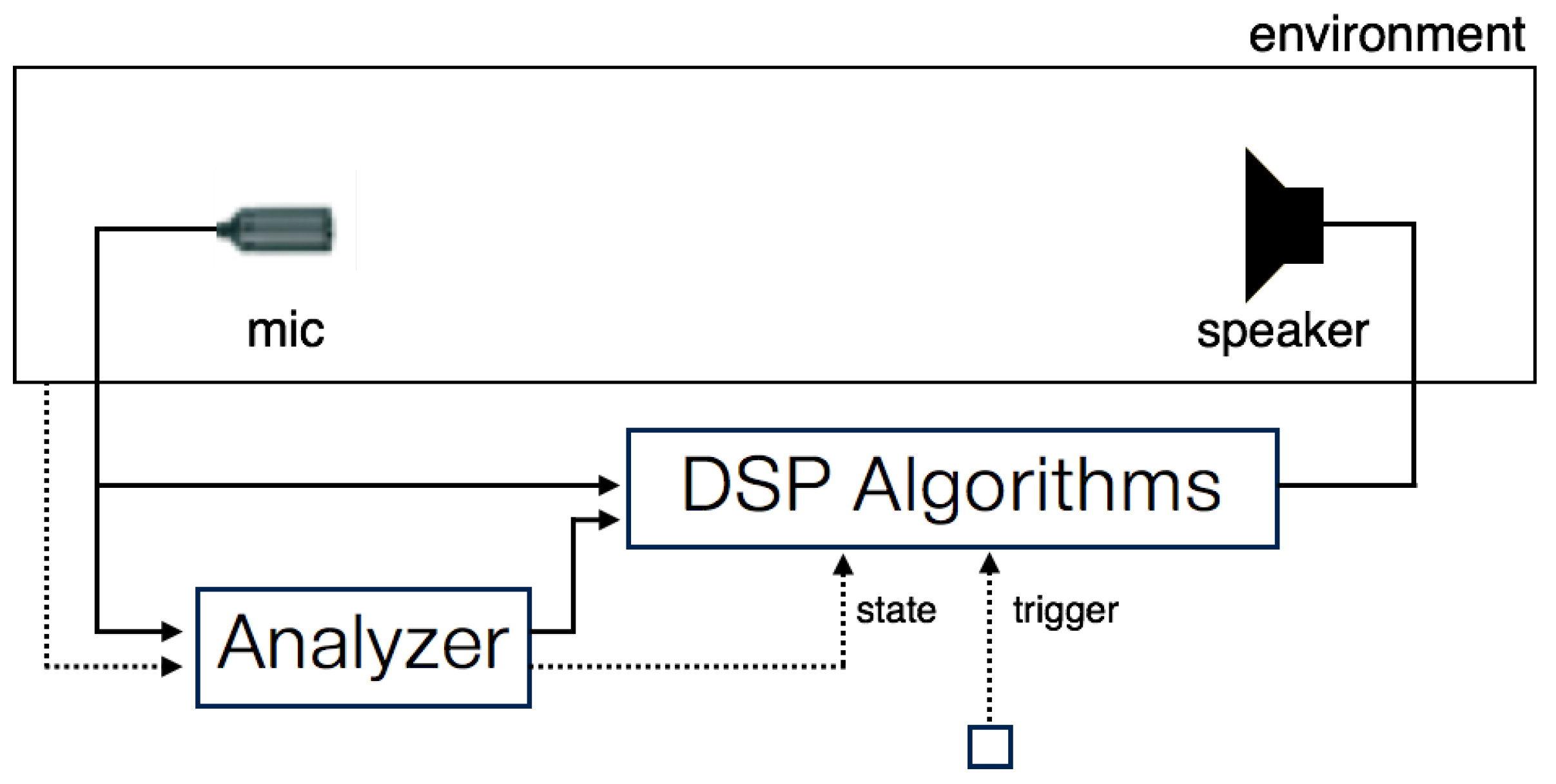
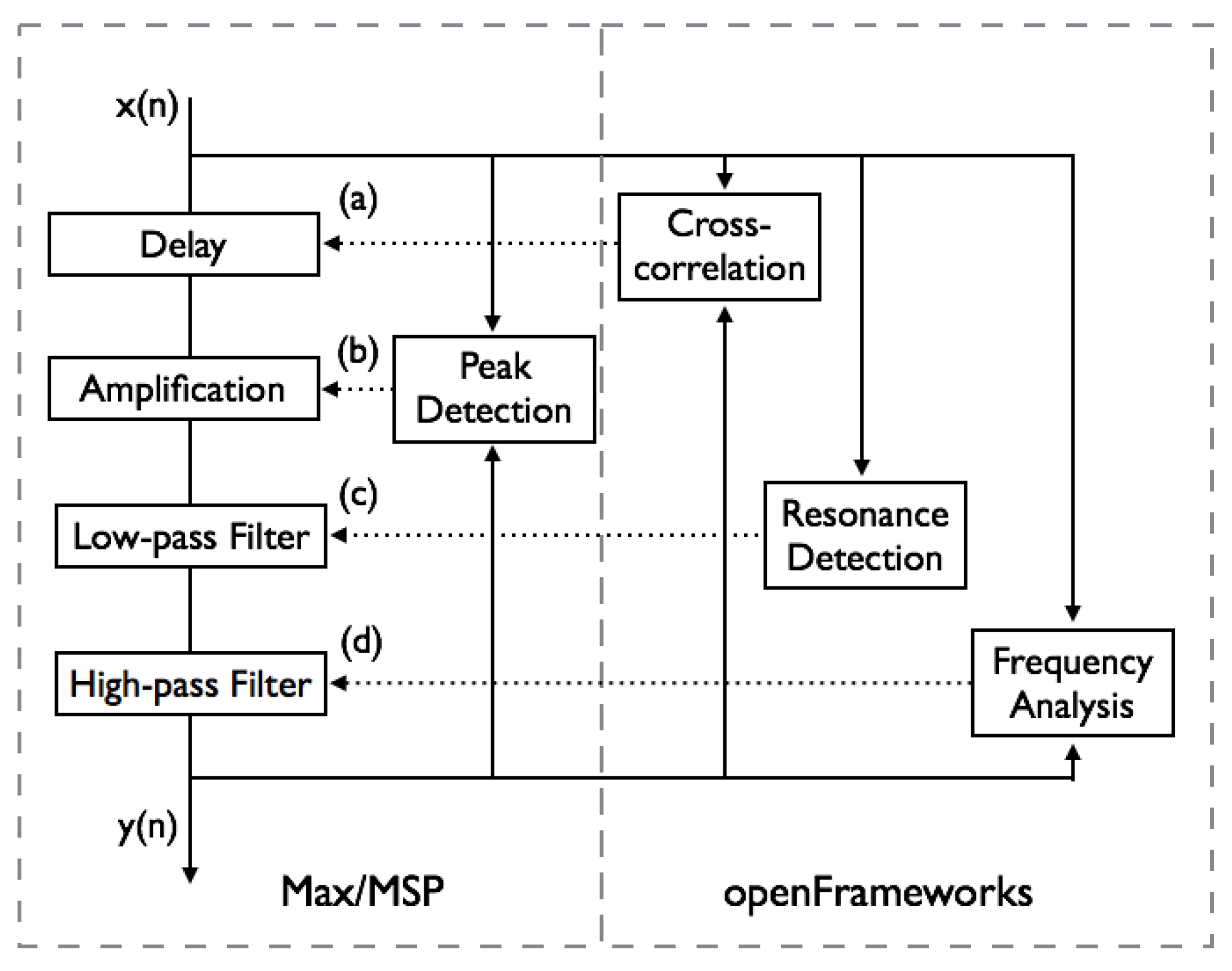
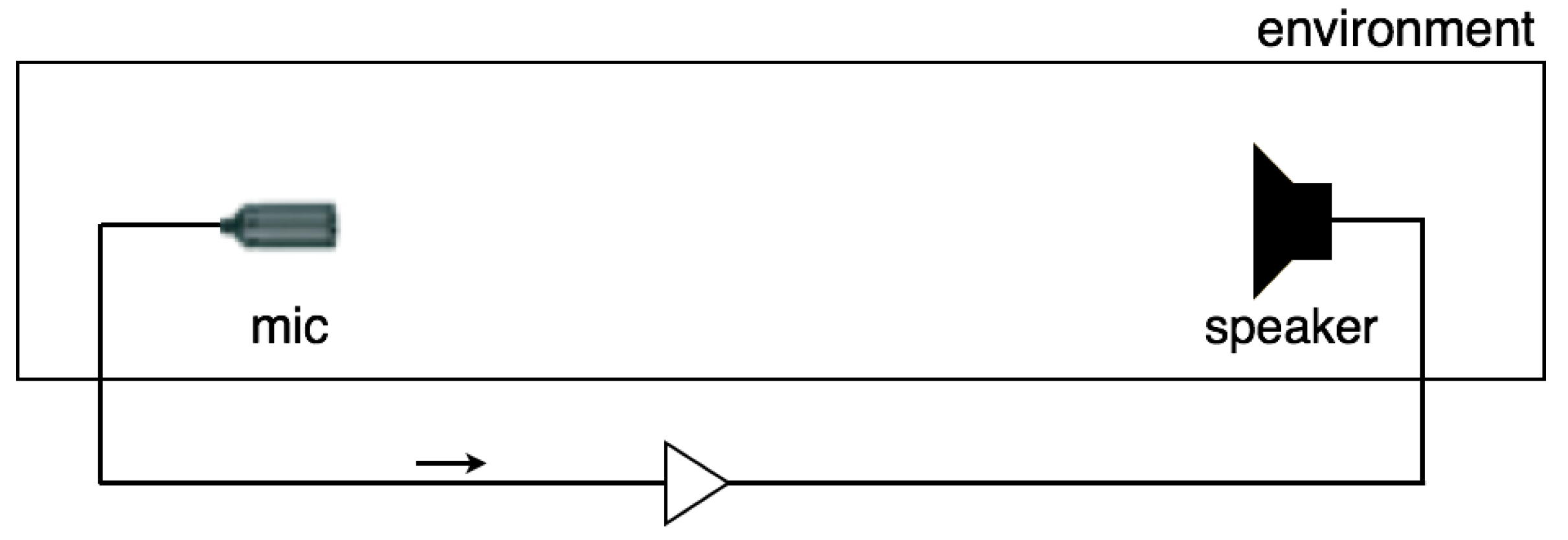
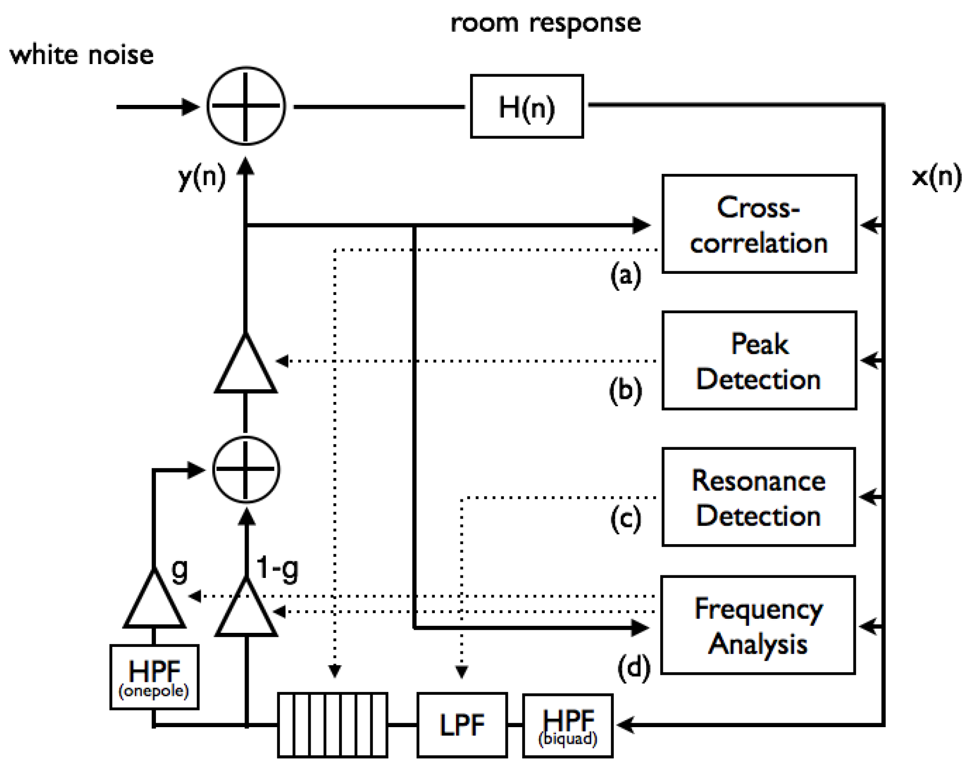
3. System Design and Validation

Based on the above notions, we designed an audio feedback system in which control of the signal-processing parameters depends on recognized features of the feedback sound, aiming in particular for sensitivity to information it carries regarding the acoustic environment. These dependencies are used to shape musical tendencies in the sonic output, with analogical approximation to the following composed interactions:

• The amount of reverberation in the space determines a tempo-scale characteristic
• The system will change its output level depending on the volume level of ambient noise
• A prominent resonance determines a timbre characteristic
• The distribution of room modes determines a timbre characteristic, energy of higher frequency partials in particular

Figure 3 shows the overall diagram for simulating the effects (tempo, volume and timbre) of audio feedback and validating the mapping. The amplifier is adaptively controlled based on the peak amplitude of the input signal. Convolution of an impulse response simulates the room acoustic response, which is shaped by propagation and reflections in physical space. We used impulse response data from Fokke van Saane [19] and Aleksey Vaneev [20]. A noise function simulates room ambient noise, used as an excitation energy source in the feedback loop. We used a biquad high-pass filter with a cutoff frequency below 80Hz to remove excessive amplification of low frequency feedback, which is uncommon in a real acoustic environment. A low-pass filter, similar to the damping loop filter of a waveguide model, is also used to reduce the howling that can be introduced by excessive amplification.

Figure 3. Overview of the system for simulating (a) tempo control by delay line length depending on room reverberation (Section 3.1), (b) volume control by gain threshold depending on volume of ambient noise (Section 3.2), (c) timbre control by cutoff frequency of a low-pass filter depending on a prominent resonance (Section 3.3) and (d) timbre control by gain of a one-pole high-pass filter according to the distribution of room modes (Section 3.4).

Table 1 compares the approximation methods and control parameters to implement the proposed mappings. It is inevitable that we can attain only approximate information about the acoustic environment from the real-time audio input, since complete real-time segregation of ambient noise and acoustic reflection information from the received feedback sound is practically impossible. Accepting this limitation, we have designed our system to infer what properties it can have, and use them to augment the specificity of the result.

Table 1. Comparison of input information, approximation methods, control targets and methods for composition of musical tendencies depending on information carried in the feedback signals regarding the acoustic environment.

Input Information	Approximation Methods	Control Targets	Control Methods
Reverberation	Cross-correlation of input/output	Tempo	Delay line length
Ambient noise volume	Peak amplitude	Output level	Gain threshold
Acoustic resonance	Freq. of maximum energy	Timbre	LPF cutoff freq.
Distribution of room modes	Variance of magnitudes	Timbre	HPF gain
	from the transfer function

3.1. Reverberation Level with Tempo

Tempo effects in the feedback sounds emerge from a combination of the adaptive gain control and the long delay line in the feedback loop. The synthesis of Larsen tones requires positive amplification of feedback, and once established, negative feedback to prevent saturation. This is achieved in our system by gradually increasing/decreasing the signal amplitude using a ramp function. The choice of amplification or de-amplification is determined by comparison of the input signal to high/low threshold values. When the peak amplitude of the signal over a three millisecond window exceeds the high threshold value (0.7), de-amplification is applied, otherwise the signal is amplified when the peak amplitude does not exceed the low threshold value (0.3). When the length of a delay line set to more than approximately 5000 samples (e.g., 100 ms), this range is more relevant to tempo-scale periodic occurrences of the Larsen tones (see Figure 4).

Figure 4. Simulated tempo-scale effects of feedback sounds when length of the delay line is (a) 22,000 samples (2 Hz) and (b) 28,500 samples (1.55 Hz). The signals are normalized to compare the tempo-scale periodic occurrences of the Larsen tones, depending on delay line length.

The cross-correlation of input x[n] with delayed output y[n] is used to derive an approximate measure of the amount of reverberation in the physical space. Cross-correlation measures the similarity between two signals as a function of time-lag, and is defined as:

$$\begin{array}{c}\hfill {\widehat{r}}_{xy}\left(l\right)=\frac{1}{N}{\displaystyle \sum _{n=0}^{N-1}}\overline{x}\left(n\right)y(n+l)\\ \hfill l=D_1,D_1+1,D_1+2,...,D_2\end{array}$$

(1)

If a sound causes strong reverberation, the reflected sound is also large and cross-correlation is expected to be high. In order to exclude direct (non-reflected) sound propagation, the cross-correlation value is taken as the mean over time-lags from 5000 (D1) to 18,000 (D2) samples (i.e., from 113 to 408 ms). This value is then divided by the maximum value over time-lags from zero to 18000 samples to minimize effect from amplitude of the feedback sound from the system. (Without this division, a louder feedback sound would also increase the cross-correlation value).

The resulting approximation of reverberation level is mapped to the length of a delay line in the feedback loop, over a range of approximately 20,000 to 55,000 samples (450 to 1250 ms). In this experiment, two opposite mappings were investigated: proportional mapping tends to generate slow tempo by a longer delay line in strongly reverberant spaces (fast tempo in weakly reverberant spaces), and reflected mapping tends to generate fast tempo by a shorter delay line in strongly reverberant spaces (slow tempo in weakly reverberant spaces). In terms of preserving the feedback signal energy, these mappings reduce or intensify the effect of the reverberant characteristics of the acoustic environment, defined as:

$$\begin{array}{cc}\hfill L_1& =a_1\times r+c_1\hfill \\ \hfill L_2& =-a_2\times r+c_2\hfill \end{array}$$

(2)

where $L_1$ and $L_2$ indicate delay line length using the proportional ($L_1$) and reflected ($L_2$) mappings, respectively, and r means cross-correlation value. The constants were chosen to achieve delay times of approximately 20,000 to 55,000 samples, such as $a_1$ = 80,000, $c_1$ = 20,000, $a_2$ = 80,000, $c_2$ = 60,000. Figure 5 evaluates the two mappings and Table 2 compares the average delay line lengths and the reverberation characteristics (RT60 and the cross-correlation values), using the impulse response data in several locations. These results affirm that the mapping results in intentional control of tendencies in audio feedback according to inferences of room reverberation.

Figure 5. Delay line length curves simulated using impulse response data of several locations with different reverberant characteristics (measured in Table 2), using the (a) proportional ($L_1$) and (b) reflected ($L_2$) mappings.

Table 2. Comparison of the reverberant characteristics measured by RT60 (the reverberation time over a 60 dB decay range), the cross-correlation values when the delay line is set to 28,000 samples, and average delay line lengths (in sample) using the proportional ($L_1$) and reflected ($L_2$) mappings.

Room Types	RT60 (s)	Xcorr	${\mathit{L}}_1$	${\mathit{L}}_2$
Livingroom	0.28	0.0407	23496	46991
Bathroom	0.58	0.1365	30674	42633
Church	0.97	0.4205	46311	30691
Long Echo Hall	3.07	0.4904	59604	25302

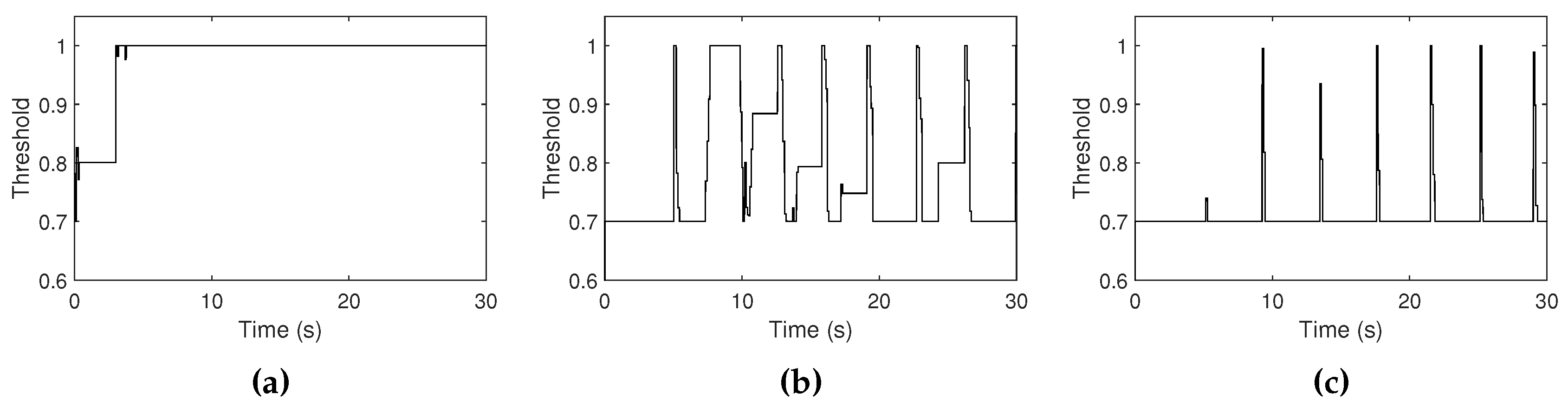
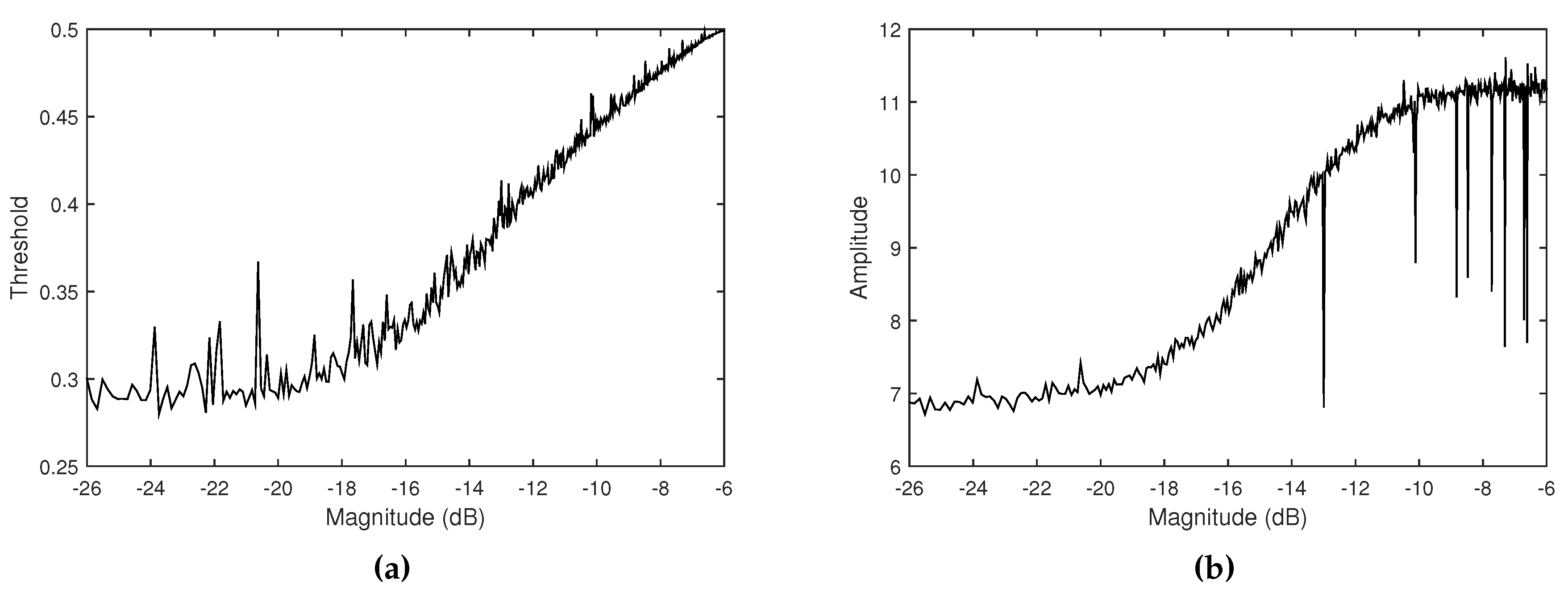
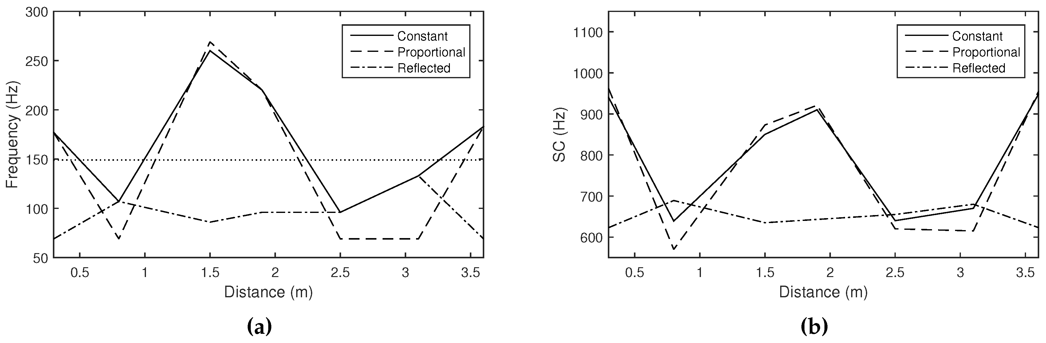
3.2. Ambient Noise Level with Amplitude Control

As mentioned in the previous Section 3.1, the adaptive gain control determines amplification or de-amplification by the high/low threshold values. In the previous tempo control, the threshold values were fixed to 0.3 and 0.7. However, use of different thresholds generates different output levels: a large threshold value tends to generate loud feedback sounds (Figure 6). The range of the thresholds are constrained between 0.2 and 1.0 to ensure the Larsen tone generation is possible.

Figure 6. Simulated amplitude control of feedback sounds when the low and high threshold values are (a) small (0.3 and 0.6) and (b) large (0.5 and 1.0). The length of the delay line is set to 30,000 samples (1.47 Hz).

In order to control the system’s output level depending on the volume level of ambient noise, the threshold values themselves are determined by measuring the amplitude of ambient noise. The threshold is updated when the amplitude of the output signal, which is measured as the maximum amplitude value in the audio frame, is below the current low threshold, in order to exclude the feedback itself from the adaptation: if the amplitude is below threshold, it is assumed that the ambient sound dominates in the input, and the threshold value is updated according to the peak amplitude of the input signal. Figure 7 compares the average threshold and peak amplitude values of the input signals according to the volume level of ambient noise, which is simulated using white noises with different amplitudes.

Figure 7. (a) Low threshold and (b) average peak amplitude curves of the feedback signals according to volume level of ambient noise. Ambient noise is simulated using different volumes of white noises.

3.3. Acoustic Resonance with Timbre

The length of the prevailing path in a feedback loop principally determines the acoustic resonance of the audio feedback, and this path is predominantly influenced by the distance between a microphone and a loudspeaker. We chose the resonant frequency as the simplest characteristic representation of acoustic resonance, and approximated it by the position of maximum energy in the spectrum. The distance between a microphone and a loudspeaker is simulated by appending a silence to the beginning of the impulse response, in order to delay the direct sound and the following reflections. Figure 8 compares the distances and the approximations of resonant frequencies.

Figure 8. Resonant frequency approximations by the position of maximum energy in the spectra of the simulated feedback signals. Distance is simulated as the length of a silence appended to the beginning of the impulse response.

Timbre, a target control feature, is the quality of sound that distinguishes different sounds of the same frequency and amplitude. Our system purposes to control timbre of the feedback sounds in terms of brightness, overall distribution of energy over frequency, by the cutoff frequency parameter of the low-pass filter. Spectral centroid is used as a measure of brightness, and Figure 9 shows the controlled different timbres through the comparison of spectra and spectral centroids: since the cutoff frequency is the attenuating position, higher cutoff frequency generates brighter sounds and lower cutoff frequency generates darker sounds.

Figure 9. Plots of the magnitude spectrum of the normalized feedback signals when the cutoff frequency of the low-pass filter is (a) 300 Hz and (b) 6000 Hz. Spectral centroids are 3327 Hz and 3965 Hz respectively. The distance is set to 4 meters.

The approximation of resonant frequency is mapped to the cutoff frequency parameter of the low-pass filter. An intriguing point is that the change in timbre (brightness) mostly influences the position of maximum energy in a spectrum, which is used as the input information. This enables evaluation of this mapping by observing changes in the approximations of resonant frequencies. However, the resonant frequency does not always behave in proportion to cutoff frequency change: timbre (brightness) may show abrupt changes by only a slight change in cutoff frequency (the nonlinearity explained in [2]). Thus, we designed the cutoff frequency to adaptively change depending on variation of the frequency approximation.

Similarly to the previous tempo control designs (Section 3.1), two opposite mappings were also investigated in accordance with the changing direction. For example, if the estimated frequency is bigger than a threshold, the cutoff frequency parameter gradually increases (proportional mapping) or decreases (reflected mapping) using a ramp function; on the other hand, when the estimated frequency is lower than a threshold, the parameter decreases (proportional mapping) or increases (reflected mapping). The effect of changing the distance is thereby intensified by the proportional mapping and reduced by the reflected mapping: Figure 10 evaluates the two mappings.

Figure 10. Approximations of spectral centroids and resonant frequencies from the simulated feedback signals when the cutoff frequency of the low-pass filter is (a,d) constant and (b,e) controlled with the proportional mapping and (c,f) reflected mappings. Vertical dot lines in the upper figures represent the positions where the approximated resonant frequencies deviate from the thresholds. These thresholds are depicted as the horizontal dot lines in the lower figures.

3.4. Distribution of Room Modes with Timbre

In Section 3.1, we approximated a measure of the amount of reverberation according to reverberation time. In this section, another approximation regarding reverberation is investigated, emphasizing related to spectral rather than of temporal characteristics. High reverberation diffusion means that reflections are scattered along various paths, producing a smooth magnitude response; on the other hand, strong reflections exist at specific frequencies in low reverberation diffusion, producing an uneven magnitude response. While in the previous Section 3.3 we measure the strongest path of audio feedback, this section is concerned with diffusion of the reflection paths.

In order to discern such distribution of room modes, we used the variance of magnitudes from the transfer function, derived from the frequency responses of the input and output signals. Table 3 compares actual measures of the distribution through spectral flatness [21] and variances from the impulse response data in several locations, and approximate measures by the variances from the derived transfer functions. Figure 11 also details these approximate measures.

Table 3. Comparison of the distributions of room modes measured by spectral flatness and variance of the magnitudes of the impulse response data ($H\left(f\right)$), average variance of the frequency magnitudes of the estimated transfer function ($H^{\prime }\left(f\right)$), and average gain values mapped by $H^{\prime }\left(f\right)$ (g).

Room Types	Spectral Flatness	Var(|$\mathit{H}(\mathit{f})$|)	Var(|${\mathit{H}}^{\prime }(\mathit{f})$|)	g
Long Echo Hall	0.85	29.71	52.90	0.56
Livingroom	0.83	31.52	61.08	0.74
Church	0.73	52.68	70.37	0.95
Bathroom	0.64	79.15	90.00	1.0

Figure 11. Variances of magnitudes of transfer functions simulated using impulse response data of several locations with different distributions of room modes (measured in Table 3).

The resulting approximation of the distribution is mapped to the gains of the unmodified output signal and a one-pole high-pass filter having a cutoff frequency of 4000 Hz, which are mixed thereafter: high variance increases the gain of the high-pass filter (decreases the gain of the unmodified signal) and the sum of the gains is always unity in linear scale. The last column in Table 3 shows the average gain values mapped by the variance measurements. This gain control changes spectral centroid as well as distribution width of spectral energy, which is associated with softness of a sound [22]. Figure 12 evaluates the mappings by comparing the changes in spectral centroids.

Figure 12. Spectral centroids measured using the impulse response data of (a) long echo hall, (b) living room, (c) church, and (d) bathroom. Solid curves represent unmodified signals, and dot curves represent output signals mixed with the output of the one-pole high-pass filter, where the mix ratio between the two signals is controlled depending on the estimated variances.

4. Experiments in a Real Room

The designed dependencies were implemented as software authored using Max/MSP 7, developed by Cycling ’74 (Santa Cruz, CA, USA) and openFrameworks, a C++ open source toolkit (Figure 13), and investigated by experiments in a 3 m × 5 m small living room with artificially controlled acoustic characteristics. Tests were performed with external audio devices 8030A loudspeaker and SM58 microphone, manufactured by Genelec (Iisalmi, Finland) and Shure (Niles, IL, USA), respectively.

Figure 13. Overview of the system implemented as software (Max/MSP and openFrameworks), for (a) tempo control depending on room reverberation (Section 4.1), (b) volume control depending on ambient noise volume (Section 4.2) and (c) timbre control depending on frequency response of the acoustic environment (Section 4.3) and (d) timbre control depending on distribution of room modes (Section 4.4).

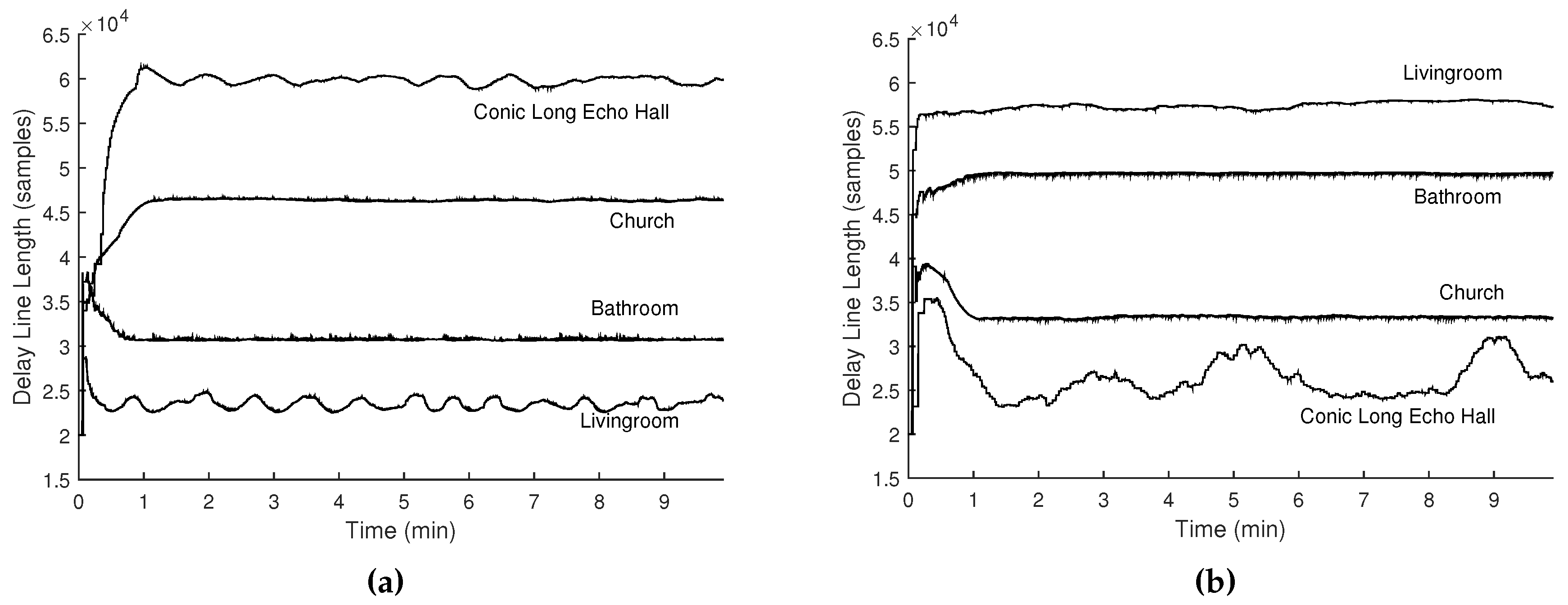
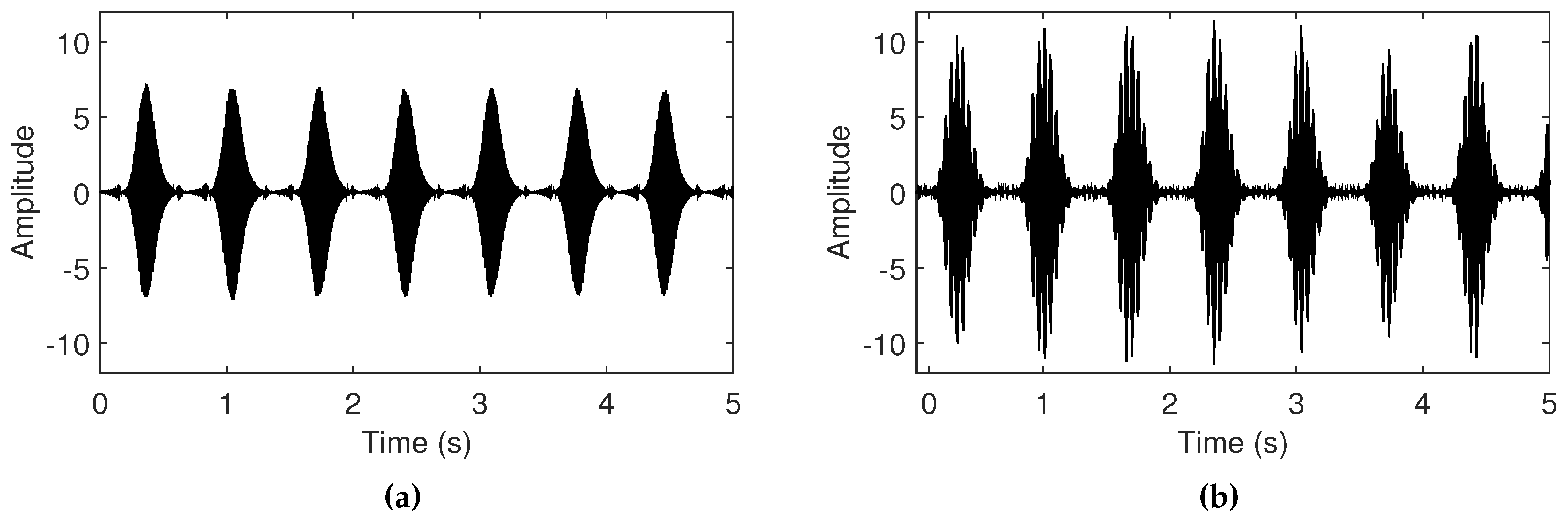
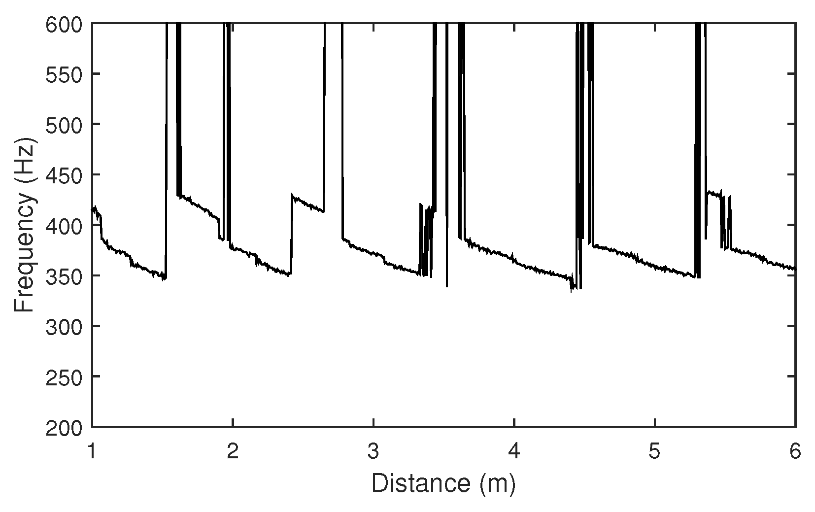
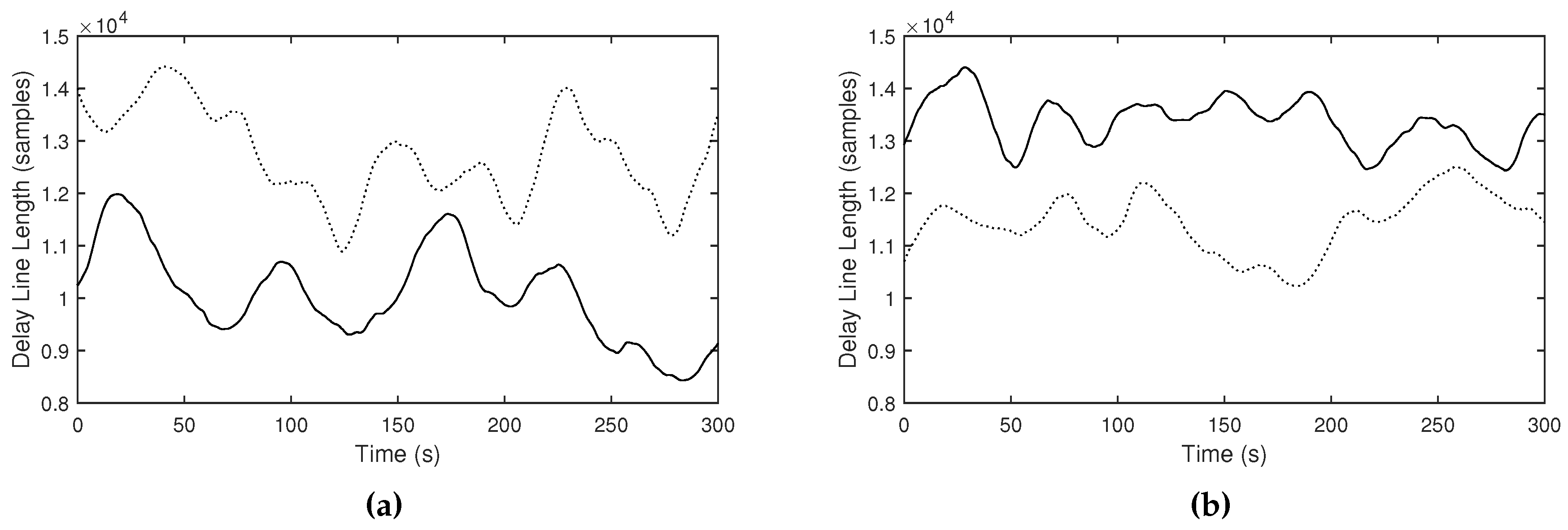
4.1. Observations in Different Room Reverberations

In the previous work, we evaluated in rooms with different reverberant acoustics, while in this paper we used a reverberation model named yafr2 that is provided within the Max/MSP software to gain more parametric control over room properties while observing changes. We experimented with different reverberation time parameters while holding other properties constant. Figure 14 and Table 4 evaluate the two mappings of delay line length from cross-correlation value. The constants in Equation (2) were chosen as $a_1$ = 33,000, $c_1$ = 1000 and $a_2$ = 33,000, $c_2$ = 20,000. Although the differences are not as clearly differentiated than those from the simulated rooms, we still observe differences in the long-term averages as expected, both when using the proportional mapping, and also with the reflected mapping.

Figure 14. Delay line length curves measured in the strongly reverberant (RT30 of 8.50 seconds, solid curves) and weakly reverberant environment (RT30 of 0.65 seconds, dot curves), using the (a) proportional ($L_1$) and (b) reflected ($L_2$) mappings.

Table 4. Comparison of the reverberant characteristics (RT30) and the average delay line lengths during the first 5 minutes, using the proportional ($L_1$) and reflected ($L_2$) mappings.

RT30 (s)	${\mathit{L}}_1$	${\mathit{L}}_2$
0.65	12720	11450
1.33	11690	11940
8.50	10070	13360

4.2. Observations in Different Ambient Noise Levels

This experiment was conducted under different ambient noise amplitudes. Figure 15 evaluates the mapping. We observed different threshold values under different noisy conditions: they increase in noisy conditions and decrease in quiet conditions, as expected.

Figure 15. High threshold curves measured when the volume level of ambient noise is measured as (a) −25 dB, (b) −30 dB, and (c) −47 dB. The range of the high threshold is constrained between 0.7 and 1.0.

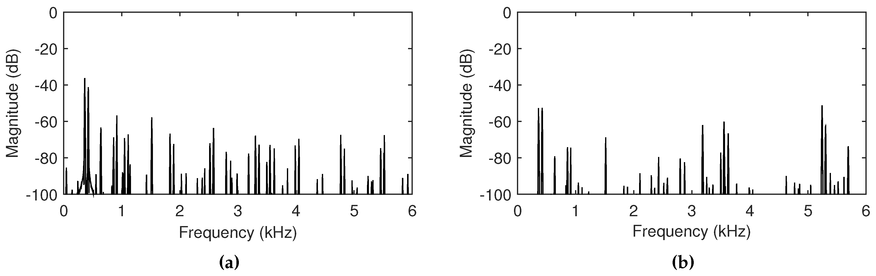
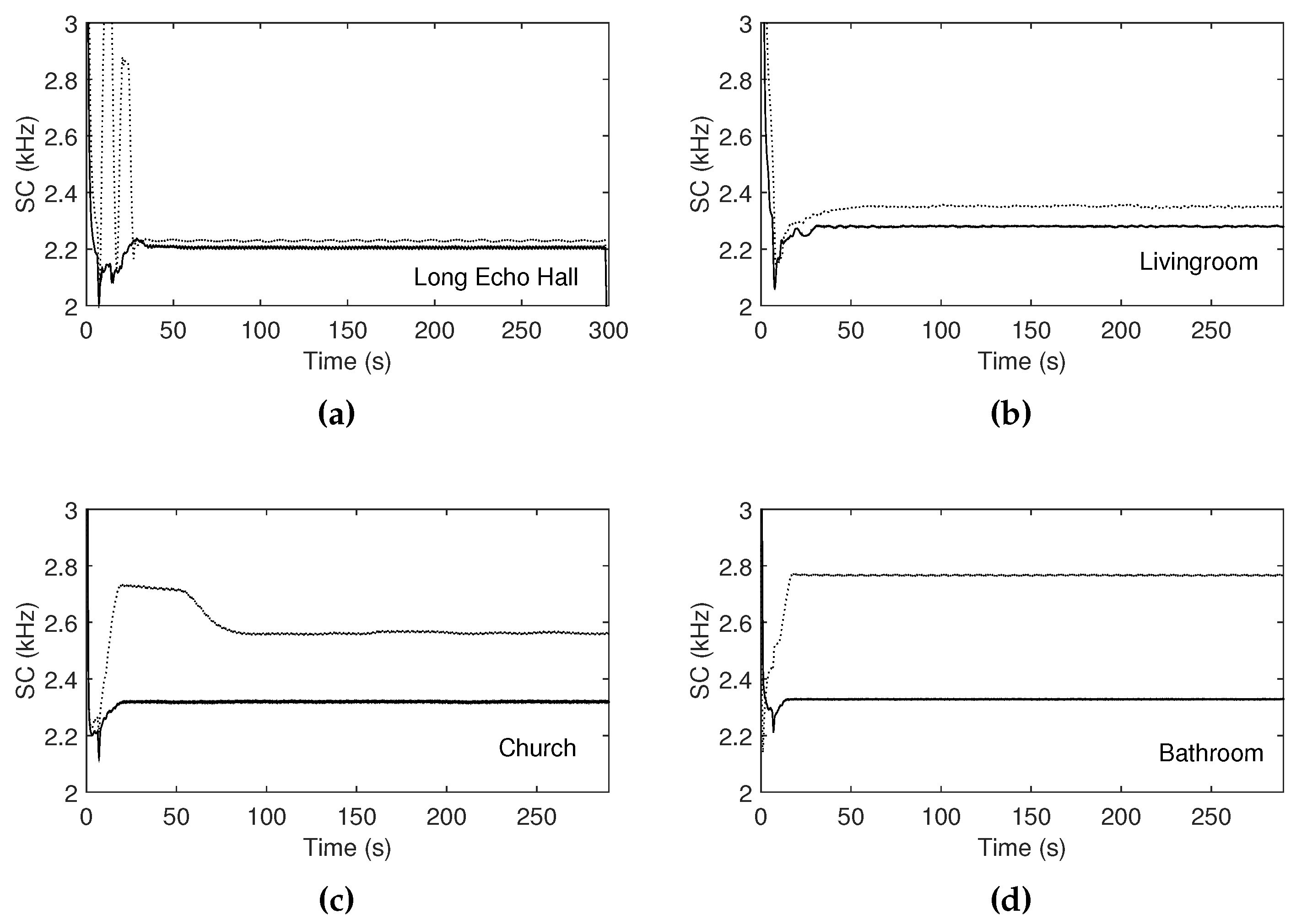
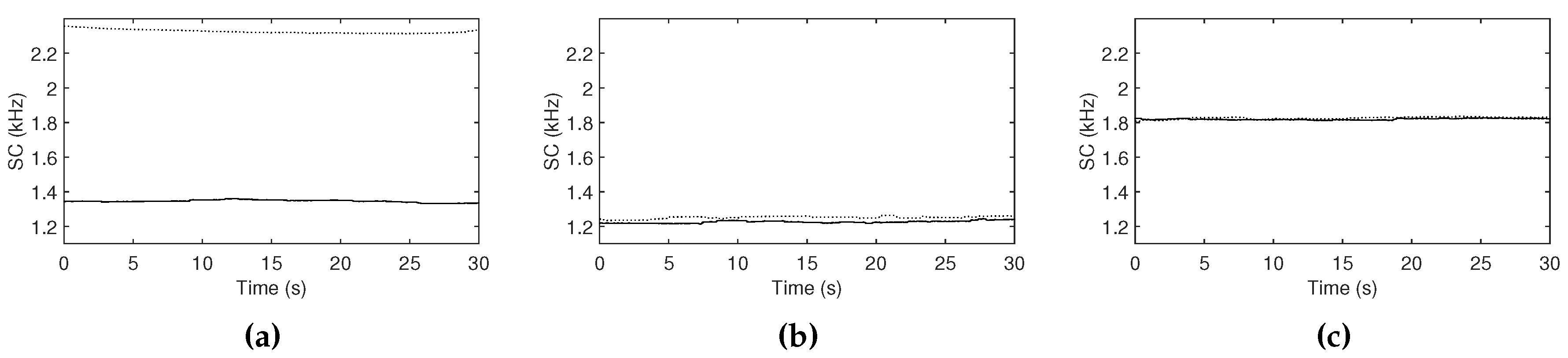
4.3. Observations with Different Acoustic Resonances

This experiment evaluated timbre changes with different distances between the microphone and the loudspeaker. Figure 16a compares the approximations of resonant frequencies using a constant or variable cutoff frequency of the low-pass filter, the latter driven by the estimated resonant frequency. We also observed the tendencies in the long-term averages as expected: the frequency change tends to be intensified by the proportional mapping and reduced by the reflected mapping. Even when the frequency is not noticeably changed, we still observed the small change in terms of brightness in comparison of the magnitude spectra (Figure 16b).

Figure 16. Approximated (a) resonant frequencies and (b) spectral centroids according to the distance between the loudspeaker and the microphone, with different cutoff frequency settings of the low-pass filter: constant (straight lines), determined by the measured resonant frequency, using the proportional ($L_1$, dash lines) and reflected mappings ($L_2$, dash-dot lines). The threshold was set to 140 Hz (dot line in (a)).

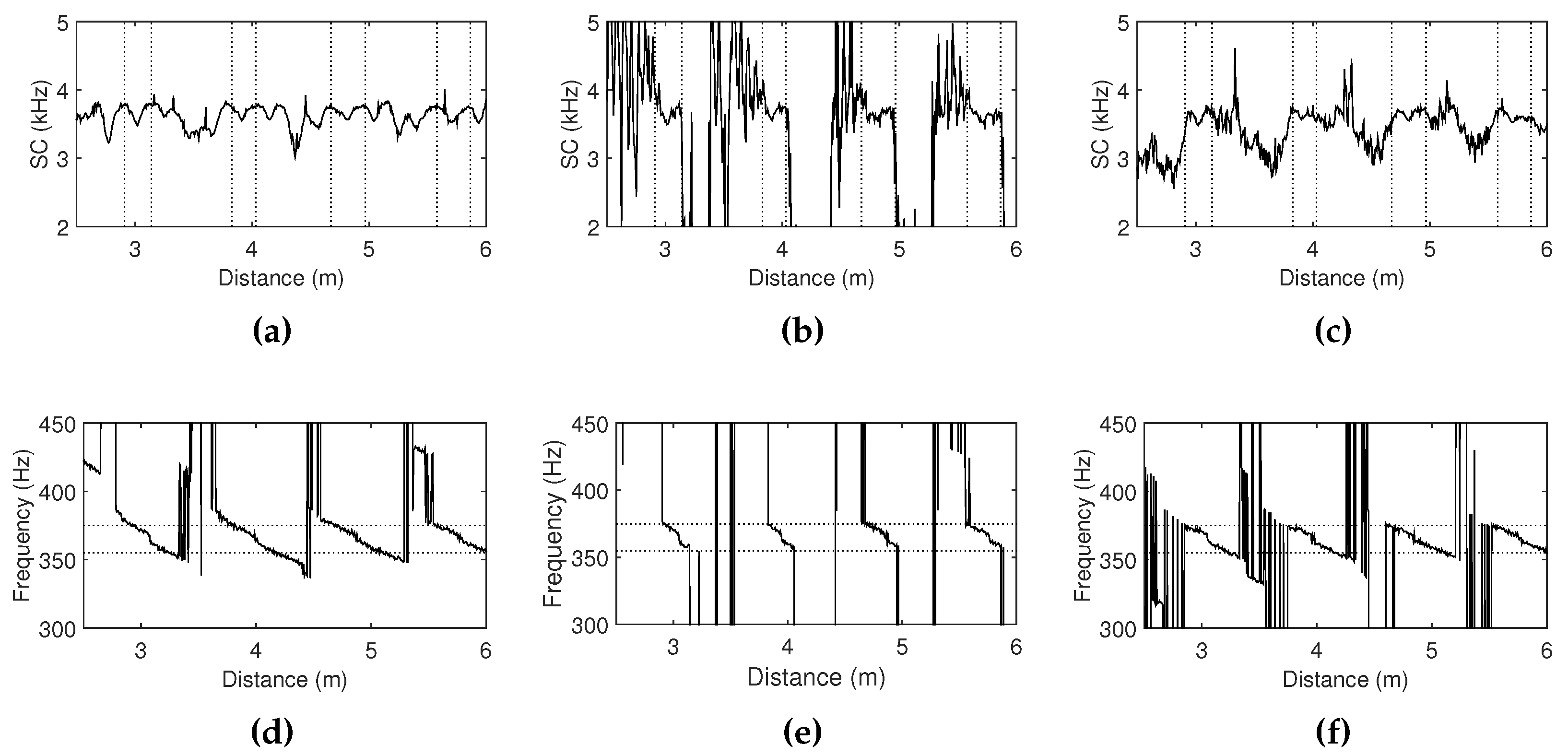
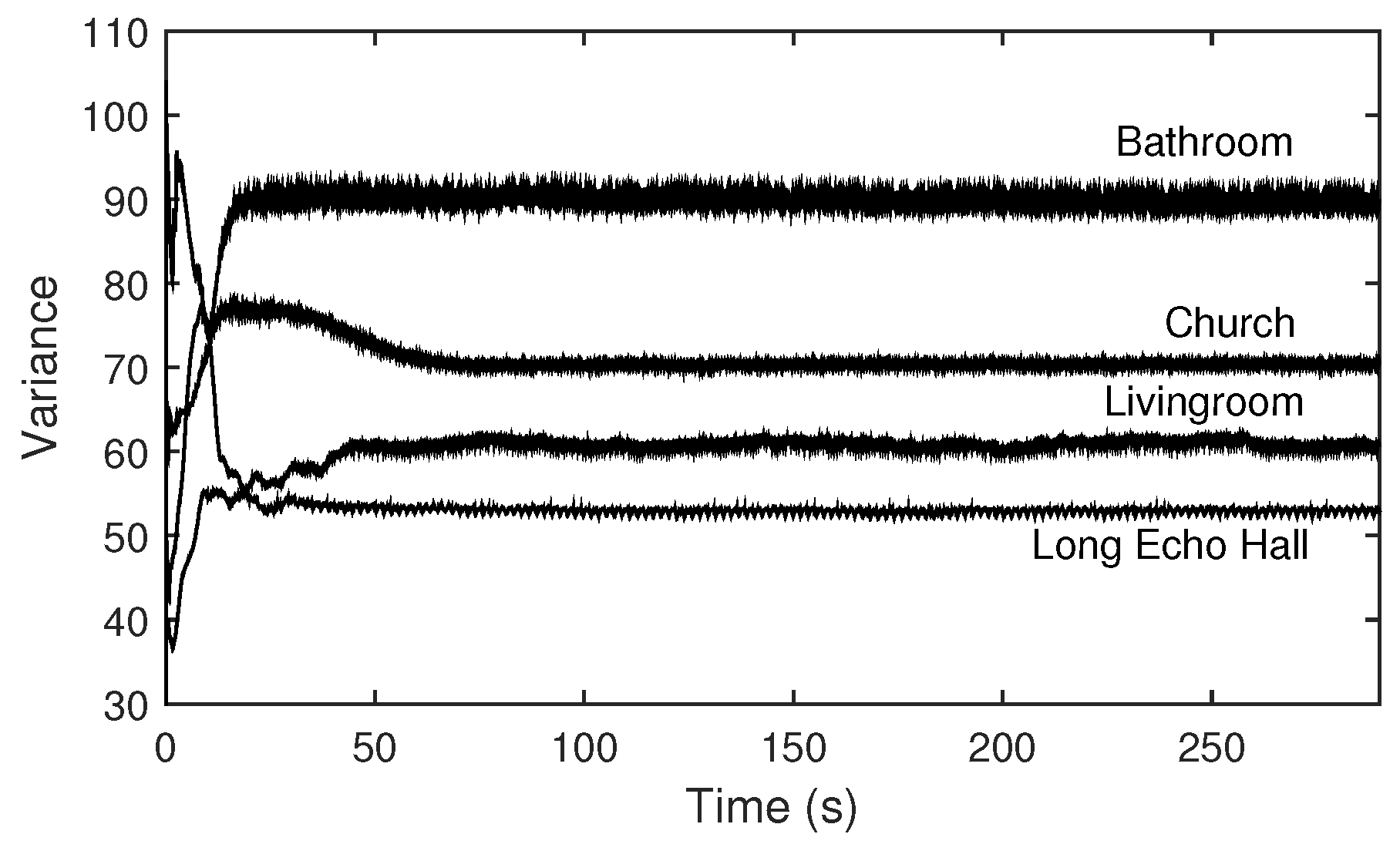
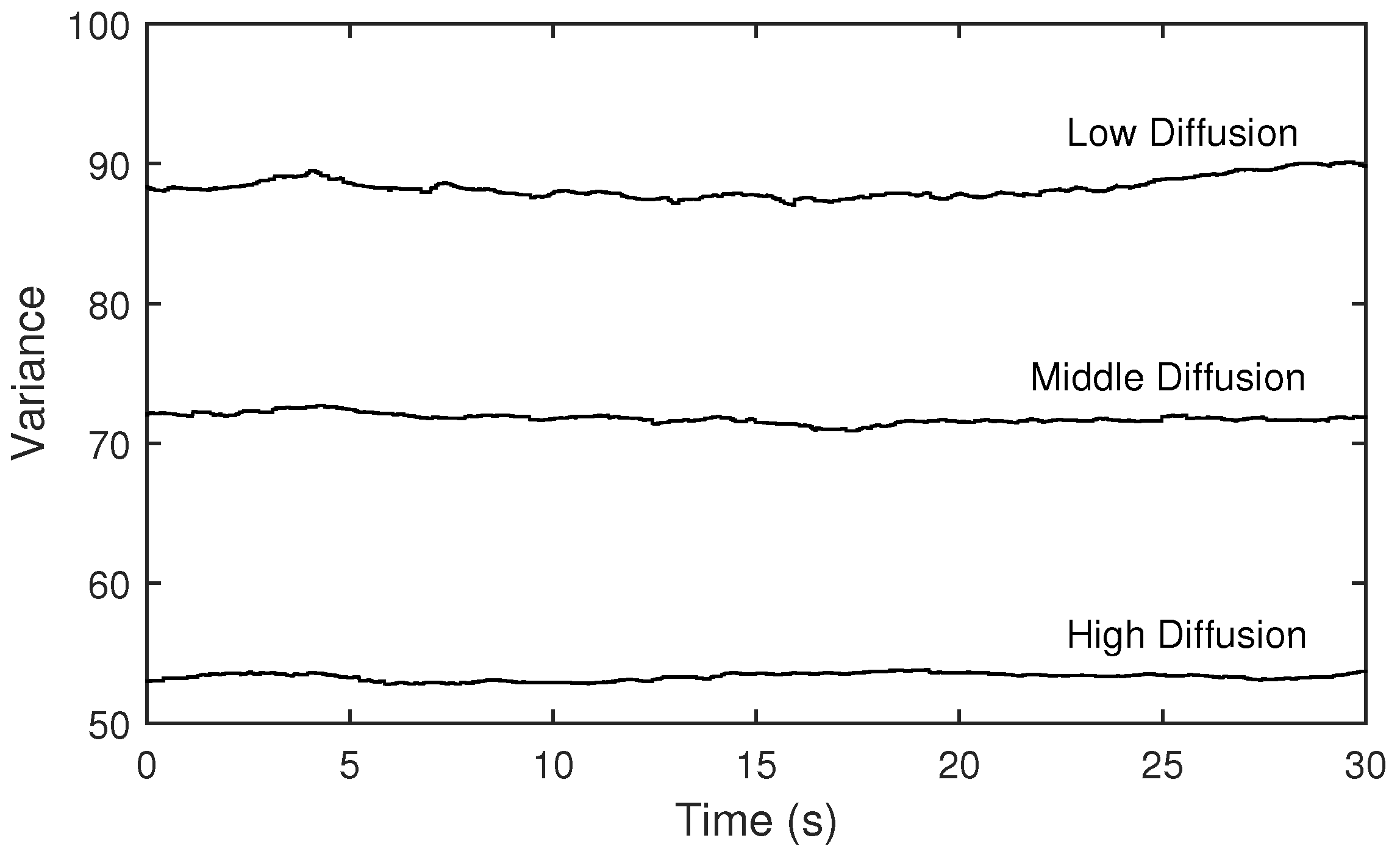
4.4. Observations with Different Distributions of Room Modes

Like the Section 4.1, different room properties are generated through diffusion parameters in the reverberation model while holding other properties constant. Figure 17 shows the measured variances and Figure 18 evaluates the mappings when the gain is constant and depends on the measurements. We also observed different variance curves and deviations of spectral centroids, as expected.

Figure 17. Variances of magnitudes of the measured transfer functions when the diffusion parameter is set to low, middle and high.

Figure 18. Spectral centroids measured when the diffusion parameter is set to (a) low, (b) middle and (c) high. Solid curves represent unmodified signals, and dot curves represent output signals mixed with the output of the one-pole high-pass filter, where the mix ratio between the two signals is controlled depending on the estimated variances.

5. Conclusions

In this paper we presented several methods for augmenting composed audio feedback interactions within acoustic environments, including room response, ambient noise and placement of transducers; supporting sound generation that strikes a balance between unpredictable short-term behavior and intentional long-term tendencies. We designed long-term tendencies in terms of tempo, amplitude and timbre characteristics depending upon reverberant properties, ambient noise level, and acoustic resonance respectively, each inferred indirectly from the environment. We measured these mappings through software simulations as well as acoustic experiments.

Beyond regarding the acoustic environment as a filter and source of disturbance, it can also be considered a site of discovery. The composed system attempts to differentiate and affirm itself through reflections, yet by doing so it also augments or exaggerates the specificity of the environment. This duality is also evident in the analysis: comparing input and output signals cannot fully segregate external and internal influence, as the feedback sounds depend upon parameters within the system, which in turn depend on the analysis. Through this paper, we are satisfied that affirming specificity was achieved, but we believe this is only an initial step in developing truly adaptive, self-augmenting responsive sonic environments.

References

1. Reich, S. Pendulum Music; Universal Editor: London, UK, 1968. [Google Scholar]
2. Sanfilippo, D.; Valle, A.; Elettronica, M. Feedback Systems: An Analytical Framework. Comput. Music J. 2013, 37, 12–27. [Google Scholar] [CrossRef]
3. Di Scipio, A. “Sound is the interface”: From Interactive to Ecosystemic Signal Processing. Organ. Sound 2003, 8, 269–277. [Google Scholar] [CrossRef]
4. Kollias, P.A. Ephemeron : Control over Self-Organised Music. In Proceedings of the 5th International Conference of Sound and Music Computing, Berlin, Germany, 31 July–3 August 2008; pp. 138–146.
5. Kim, S.; Nam, J.; Wakefield, G. Toward Certain Sonic Properties of an Audio Feedback System by Evolutionary Control of Second-Order Structures. In Proceedings of the 4th International Conference (and 12th European event) on Evolutionary and Biologically Inspired Music, Sound, Art and Design (Part of Evostar 2015), Copenhagen, Denmark, 8–10 April 2015.
6. Berdahl, E.; Harris, D. Frequency Shifting for Acoustic Howling Suppression. In Proceedings of the 13th International Conference on Digital Audio Effects, Graz, Austria, 6–10 September 2010.
7. Gabrielli, L.; Giobbi, M.; Squartini, S.; Valimaki, V. A Nonlinear Second-Order Digital Oscillator for Virtual Acoustic Feedback. In Processing of the 2014 IEEE International Conference on Acoustics, Speech and Signal Processing (ICASSP), Florence, Italy, 4–9 May 2014; pp. 7485–7489.
8. Karjalainen, M.; Välimäki, V.; Tolonen, T. Plucked-String Models: From the Karplus-Strong Algorithm to Digital Waveguides and Beyond. Comput. Music J. 1998, 17–32. [Google Scholar] [CrossRef]
9. Kim, S.; Kim, M.; Yeo, W.S. Digital Waveguide Synthesis of the Geomungo with a Time-varying Loss Filter. J. Audio Eng. Soc. 2013, 61, 50–61. [Google Scholar]
10. Smith, J.O. Physical Modeling using Digital Waveguides. Comput. Music J. 1992, 16, 74–91. [Google Scholar] [CrossRef]
11. Sullivan, C.R. Extending the Karplus-Strong Algorithm to Synthesize Electric Guitar Timbres with Distortion and Feedback. Comput. Music J. 1990, 14, 26–37. [Google Scholar] [CrossRef]
12. Gustafsson, F. System and Method for Simulation of Acoustic Feedback. US Patent 7,572,972, 2009. [Google Scholar]
13. Waters, S. Performance Ecosystems: Ecological Approaches to Musical Interaction. EMS: Electroacoustic Music Studies Network, 2007; pp. 1–20. [Google Scholar]
14. Overholt, D.; Berdahl, E.; Hamilton, R. Advancements in Actuated Musical Instruments. Organ. Sound 2011, 16, 154–165. [Google Scholar] [CrossRef]
15. Kollias, P.A. The Self-Organising Work of Music. Organ. Sound 2011, 16, 192–199. [Google Scholar] [CrossRef]
16. Scamarcio, M. Space as an Evolution Strategy. Sketch of a Generative Ecosystemic Structure of Sound. In Proceedings of the Sound and Music Computing Conference, Berlin, Germany, 31 July–3 August 2008; pp. 95–99.
17. Di Scipio, A. Listening to Yourself through the Otherself: On Background Noise Study and Other Works. Organ. Sound 2011, 16, 97–108. [Google Scholar] [CrossRef]
18. Aufermann, K. Feedback and Music: You Provide the Noise, the Order Comes by Itself. Kybernetes 2005, 34, 490–496. [Google Scholar] [CrossRef]
19. Impulse Responses Made by Fokke van Saane. Available online: http://fokkie.home.xs4all.nl/IR.htm (accessed on 23 April 2016).
20. Free Reverb Impulse Responses. Available online: http://www.voxengo.com/impulses (accessed on 23 April 2016).
21. Lerch, A. An Introduction to Audio Content Analysis: Applications in Signal Processing and Music Informatics; John Wiley & Sons: New York, NY, USA, 2012. [Google Scholar]
22. Fritz, C.; Blackwell, A.F.; Cross, I.; Woodhouse, J.; Moore, B.C. Exploring Violin Sound Quality: Investigating English Timbre Descriptors and Correlating Resynthesized Acoustical Modifications with Perceptual Properties. J. Acoust. Soc. Am. 2012, 131, 783–794. [Google Scholar] [PubMed]
Article Metrics
Citations
Article Access Statistics
Multiple requests from the same IP address are counted as one view.