Pore-Scale Evolution of Effective Properties in Porous Rocks During Dissolution/Erosion and Precipitation

Abstract

Reactive transport in porous media exists ubiquitously in natural and industrial systems—reformation of geological energy repository, carbon dioxide (CO₂) sequestration, CO₂ storage via mineralization, and soil remediation are just some examples where geo-/bio-chemical reactions play a key role. Reactive transport models are expected to provide assessments of (1) the effective property variation and (2) the reaction capability. However, the synergy among flow, solute transport, and reaction undermines the predictability of the existing model. In recent decades, the Micro-Continuum Approach (MCA) has demonstrated advantages for modeling pore-scale reactive transport and high accuracy compared with experiments. In this study, we present an MCA-based numerical framework that simulates dissolution/erosion or precipitation in digital rocks. The framework imports two- or three-dimensional digital rock samples, conducts reactive transport simulations, and evaluates dynamic changes in porosity, surface area, permeability tensor, tortuosity, mass change, and reaction rate. The results show that samples with similar effective properties, e.g., porosity or permeability, may exhibit different reaction abilities, suggesting that the pore-scale geometry has a strong impact on reactive transport. Additionally, the numerical framework demonstrates the advantage of conducting multiple reaction studies on the same sample, in contrast to reality, where there is often only one physical experiment. This advantage enables the identification of the optimal condition, quantified by the dimensionless Péclet number and Damköhler number, to reach the maximum reaction. We believe that the newly developed framework serves as a toolbox for evaluating reactivity capacity and predicting effective properties of digital samples.

1. Introduction

Chemical and bio- and geo-chemical reactions occur in various subsurface systems, including natural and industrial ones. Some examples include carbon dioxide mineralization in basaltic formation [1,2], acidization of shale [3,4], remediation of soil [5,6,7], bio-film growth [8,9], and rare earth element recovery [10,11,12]. The Fluid–Rock reaction is one of the vital processes, if not the decisive one, in the application scenarios mentioned above. Thus, reactive transport modeling has attracted researchers’ attention for decades.

Two types of reactions occur ubiquitously: (1) dissolution, i.e., the solid phase is dissolved by a substance (e.g., acid, organic solvent, microbios, etc.) in the fluid and leaves the void space [13,14,15], and (2) precipitation, i.e., the new solid phase precipitates on the existing mineral surface. In general, dissolution and precipitation in a subsurface system involve a complex chain of reactions; a different set of reactions may occur when conditions (e.g., pH) shift. These reactions are intertwined with fluid flow and solute transport in addition to the heterogeneity of the media [16,17,18]. Moreover, dissolution and/or precipitation reactions dynamically change the pore geometry; as a consequence, the macroscopic flow and transport properties, such as porosity, permeability, and tortuosity, are also dynamic. Additionally, the inherent multiscale nature of the porous media in subsurface system layers adds extra complexity to the modeling task.

Digital rocks are frequently utilized to study subsurface formations. With the fast development of experimental techniques and characterization tools, compositional and geometrical information [19,20,21] can be digitalized and used for numerical investigation. For a given digital rock sample, evaluating the macroscopic property and predicting the reaction capability are two major tasks for reactive transport models. Review papers [22,23,24,25] provide detailed information from several perspectives: reactive transport mechanism and modeling, fluid–rock reaction modeling, parameter estimation, pore-scale numerical models, and benchmark experiments. Among reactive transport models, the Micro-Continuum Approach (MCA) has gained attention in recent years. Early development of MCA was performed by Steefel and co-workers [23,26]. Soulaine et al. conducted a series of studies [27,28] in which they implemented an MCA solver and rigorously validated it by comparing numerical results with experiments. Later, Soulaine et al. extended the single-phase MCA to a multiphase scenario [29]. A detailed review, comparison of the MCA-based method and other reactive transport methods, and benchmark experiment can be found in the study by Molins and et al. [25]. Recent advances have extended the MCA to several areas, including the Lattice Boltzmann framework [30], coupling with the Discrete Element Method [31], and other aspects of subsurface process modeling [32].

The MCA considers that the domain is composed of microscopic continua whose properties are determined by the volume fraction of each phase. The interface between the fluid phase (or pore space) and the solid phase is represented by a continuous variation in volume fraction rather than a sharp jump. Two advantages of the MCA are (1) the flow field of both fluid and solid regions can be solved with a unified equation, and (2) the continuity of the phase volume fraction across the fluid–solid interface does not require re-meshing or local refinement during simulation. With these advantages, MCA is an ideal method to investigate reactive transport in samples with complex interfaces, e.g., digital rocks. In this study, we implement an MCA-based reactive transport solver in the OpenFOAM environment and combine the solver with macroscopic property evaluation modules, forming a numerical framework. The framework simulates dissolution/precipitation reactions in digital rock samples and computes macroscopic properties of the pore geometry output via the reactive solver.

The following macroscopic properties are computed at every time instance: porosity, surface area, permeability, tortuosity, mass, and reaction rate. These properties are essential for assessing the reaction’s impact on the pore geometry and/or predicting the reaction capacity of a given sample. For instance, in the CO₂ sequestration application, dissolution may change the cap rock’s permeability [33], leading to leakage. As another example, accurate prediction of precipitated mass and precipitation rate can assist in evaluating carbon storage sites [34]. As for the numerical modeling aspect, accurate estimation of the effective properties of a micro-scale sample enhances the predictive power of a macro-scale model that uses them as model parameters [35].

Pre-processing and post-processing algorithms are also embedded in the framework, which enable the importation of segmented digital rock samples. Unlike reactive transport experiments, which can test a sample only once, numerical simulation allows trials of different flow and reaction conditions on the same sample. Such capacity provides a means to identify the optimal flow and transport region where the reaction reaches its maximum. Additionally, our results show that the reacted mass and the reaction rate are not monotonic functions of the initial porosity/permeability, indicating that an optimization test is needed to achieve maximum reactivity.

Overall, the new framework provides a numerical tool for assessing dissolution or precipitation reactions and their impact on flow and transport properties. Also, the compatibility with digital rock samples widens the applicability of the MCA methods in subsurface systems and provides an effective platform for parameter calculation and multi-scale/upscale computation. This paper is organized as follows: Section 1 presents a brief overview of the MCA method and introduction of the new framework. Section 2 lists all the equations used in the MCA, followed by formulas of all the macroscopic properties. Section 3 introduces the workflow of the numerical framework and the pre-/post-processing algorithms used in the study. Section 4 presents numerical results from both two- and three-dimensional studies; physical insights; detailed analysis; and the exploration of the synergy between flow, transport, and reaction. Section 5 concludes the paper and discusses a few potential directions of our future work.

2. Formulation

Unlike conventional pore-scale modeling, where the fluid and solid domains are distinctly defined, the MCA assumes that each point in the domain is a micro-continuum consisting of both fluid and solid. Consequently, the boundary between fluid and solid is no longer a sharp interface; instead, it is delineated by the volume fraction of each phase. A detailed formulation can be found in literature [25,26,27]. The flow field of the entire domain, including both fluid and solid portions, is solved by the Darcy–Brinkman–Stokes Equation (DBSE):

$$\begin{array}{c}\hfill {\displaystyle \frac{1}{{\epsilon }_{\mathrm{f}}}}\left[{\displaystyle \frac{\partial {\rho }_{\mathrm{f}}\mathbf{u}}{\partial t}}+\nabla ·\left({\displaystyle \frac{{\rho }_{\mathrm{f}}}{{\epsilon }_{\mathrm{f}}}}\mathbf{u}\mathbf{u}\right)\right]=-\nabla p+{\displaystyle \frac{\mu }{{\epsilon }_{\mathrm{f}}}}{\nabla }^2\mathbf{u}-\mu R\mathbf{u},\end{array}$$

(1)

where ${\epsilon }_{\mathrm{f}}$ [-] is the volume fraction of the fluid, ${\rho }_{\mathrm{f}}$ [kg·m⁻³] is the density of the fluid, $\mathbf{u}$ [m·s⁻¹] is the velocity vector, p [kg·m⁻¹·s⁻²] is the pressure, $\mu$ [kg·m⁻¹·s⁻¹] is the viscosity, and the flow resistance R [m⁻²] is the inverse of the permeability (k [m²]):

$$\begin{array}{c}\hfill R={\displaystyle \frac{1}{k}}.\end{array}$$

(2)

Importantly, the flow resistance R and permeability k in Equations (1) and (2) are scalars and defined point-wise. The volume fraction of the solid is denoted as ${\epsilon }_{\mathrm{s}}$, and the following relationship holds:

$$\begin{array}{c}\hfill {\epsilon }_{\mathrm{f}}+{\epsilon }_{\mathrm{s}}=1.\end{array}$$

(3)

The porosity of every micro-continuum is equivalent to the volume fraction of fluid: $\varphi ={\epsilon }_{\mathrm{f}}$. A constitutive relation associating micro-continua porosity and flow resistance is needed; for instance, the Kozeny–Carman equation [25,27]:

$$\begin{array}{c}\hfill R=R_{\mathrm{o}}{\displaystyle \frac{{\left(1-{\epsilon }_{\mathrm{f}}\right)}^2}{{\epsilon }_{\mathrm{f}}^3}},\end{array}$$

(4)

where $R_{\mathrm{o}}$ [m⁻²] is a reference resistance.

Solute transport is modeled using the Advection Diffusion Reaction Equation (ADRE):

$$\begin{array}{c}\hfill {\displaystyle \frac{\partial {\epsilon }_f\mathrm{c}}{\partial t}}+\nabla \left(\mathbf{u}\mathrm{c}\right)=\nabla ·\left({\epsilon }_f{\mathrm{D}}^{*}\nabla \mathrm{c}\right)-\xi {\mathrm{c}}_0{r}_{\mathrm{t}},\end{array}$$

(5)

where $\mathrm{c}$ [mol· m⁻³] is the concentration of the solute; ${\mathrm{D}}^{*}$ [m² · s⁻¹] is the effective diffusion coefficient of the solute; $r_{\mathrm{t}}$ [s⁻¹] is the reaction rate; ${\mathrm{c}}_0$ is the reference concentration, which is assumed to be ${\mathrm{c}}_0=1$ mol·m⁻³; and $\xi$ [-] is the stoichiometric coefficient of the solute. A constitutive relationship [26] for the diffusion coefficient is also used:

$$\begin{array}{c}\hfill D^{*}={\epsilon }_{\mathrm{f}}{D}_{\mathrm{f}}.\end{array}$$

(6)

where $D_{\mathrm{f}}$ [m² · s⁻¹] are the diffusion coefficients in the fluid. The reaction rate is computed

$$\begin{array}{c}\hfill r_{\mathrm{t}}=\alpha {\displaystyle \frac{\mathrm{c}}{{\mathrm{c}}_0}}\left({\epsilon }_{\mathrm{s},\mathrm{eq}}-{\epsilon }_{\mathrm{s}}\right)\left|\nabla {\epsilon }_{\mathrm{f}}\right|L,\end{array}$$

(7)

where $\alpha$ [s⁻¹] is the constant reaction rate, ${\epsilon }_{\mathrm{s},\mathrm{eq}}$ is the equilibrium solid volume fraction, $\left|\nabla {\epsilon }_{\mathrm{f}}\right|$ [m⁻¹] is the surface area per unit volume, and L [m] is the characteristic length scale of the domain. In Equation (7), when ${\epsilon }_{\mathrm{s},\mathrm{eq}}<{\epsilon }_{\mathrm{s}}$, the solid phase dissolves (i.e., $r_{\mathrm{t}}<0$), and the solute precipitates (i.e., $r_{\mathrm{t}}>0$) when ${\epsilon }_{\mathrm{s},\mathrm{eq}}>{\epsilon }_{\mathrm{s}}$. The primary assumptions are (1) a single, first-order kinetic rate law for the surface reaction and (2) constant diffusion coefficients for the solute species. The volume of solid variation according to the reaction is modeled by

$$\begin{array}{c}\hfill {\displaystyle \frac{\partial {\epsilon }_{\mathrm{s}}}{\partial t}}=r_{\mathrm{t}}.\end{array}$$

(8)

The continuity equation is now

$$\begin{array}{c}\hfill \nabla ·\mathbf{u}=r_{\mathrm{t}}\left({\displaystyle \frac{{\rho }_{\mathrm{s}}}{{\rho }_{\mathrm{f}}}}-1\right).\end{array}$$

(9)

where ${\rho }_{\mathrm{s}}$ [kg·m⁻³] is the density of the solid. The solution of (1)–(9) provides the temporal evolution of the flow, solute, and fluid–solid phase in the domain. In this study, we define three characteristic time scales:

$$\begin{array}{c}\hfill T_a={\displaystyle \frac{L}{U_0}},T_d={\displaystyle \frac{L^2}{D_{\mathrm{f}}}},T_r={\displaystyle \frac{1}{\alpha }},\end{array}$$

(10)

Here, $T_a$ denotes the advection time scale, $T_d$ is the diffusion time scale, $T_r$ is the reaction time scale, and $U_0$ is the velocity scale. By taking the ratio of two time scales, we reach the definition of two dimensionless numbers:

$$\begin{array}{c}\hfill \mathit{Pe}={\displaystyle \frac{T_d}{T_a}}={\displaystyle \frac{L{U}_0}{D_{\mathrm{f}}}},{\mathit{Da}}_I={\displaystyle \frac{T_a}{{\tau }_r}}={\displaystyle \frac{\alpha L}{U_0}},{\mathit{Da}}_{II}={\displaystyle \frac{T_d}{{\tau }_r}}={\displaystyle \frac{\alpha L^2}{D_{\mathrm{f}}}}.\end{array}$$

(11)

$\mathit{Pe}$ is the Péclet number, and ${\mathit{Da}}_I$ and ${\mathit{Da}}_{II}$ are Damköhler numbers for advection and diffusion, respectively. We use the dimensionless number to quantify and study our reactive cases.

In this study, we perform dissolution/precipitation simulations using three-dimensional digital rock samples. In Cartesian coordinates, the domain of interest is bounded: $\mathsf{\Omega }\in \left[0,L\right]\times \left[0,L\right]\times \left[0,L\right]$, where $\mathsf{\Omega }$ [m³] denotes the entire domain, including the fluid ${\mathsf{\Omega }}_{\mathrm{f}}$ [m³] and solid ${\mathsf{\Omega }}_{\mathrm{s}}$ [m³]. To illustrate, a two-dimensional example is shown in Figure 1. The reactive fluid is injected from $x=0$ at a constant velocity, and a zero-gradient condition is applied to the pressure. At the outlet ($x=L$), a reference pressure condition is imposed, ${p|}_{x=L}=0$, while the velocity and concentration fields respect the zero gradient condition. At the side boundaries ($y=\{0,L\}$ and $z=\{0,L\}$), the no-slip condition is enforced, and the zero-gradient condition is applied to the pressure and concentration. To summarize, the boundary conditions at the inlet are as follows:

$$\mathbf{u}{|}_{x=0}=\left(U_0,0,0\right),$$

(12)

$${\displaystyle \frac{\partial \mathrm{p}}{\partial \mathbf{n}}}{|}_{x=0}=0,$$

(13)

$$\mathrm{c}{|}_{x=0}=c_0,$$

(14)

On the side boundaries:

$${\displaystyle \frac{\partial \mathbf{u}}{\partial \mathbf{n}}}{|}_{y=\left\{0,L\right\},z=\left\{0,L\right\}}=\mathbf{0},$$

(15)

$${\displaystyle \frac{\partial \mathrm{p}}{\partial \mathbf{n}}}{|}_{y=\left\{0,L\right\},z=\left\{0,L\right\}}=0,$$

(16)

$${\displaystyle \frac{\partial \mathrm{c}}{\partial \mathbf{n}}}{|}_{y=\left\{0,L\right\},z=\left\{0,L\right\}}=0,$$

(17)

At the outlet:

$${\displaystyle \frac{\partial \mathbf{u}}{\partial \mathbf{n}}}{|}_{z=L}=\mathbf{0},$$

(18)

$$\mathrm{p}{|}_{x=L}=0,$$

(19)

$${\displaystyle \frac{\partial \mathrm{c}}{\partial \mathbf{n}}}{|}_{x=L}=0.$$

(20)

Initial conditions are as follows:

$$u{|}_{t=0}=\mathbf{0},$$

(21)

$$p{|}_{t=0}=0,$$

(22)

$$c{|}_{t=0}=0.$$

(23)

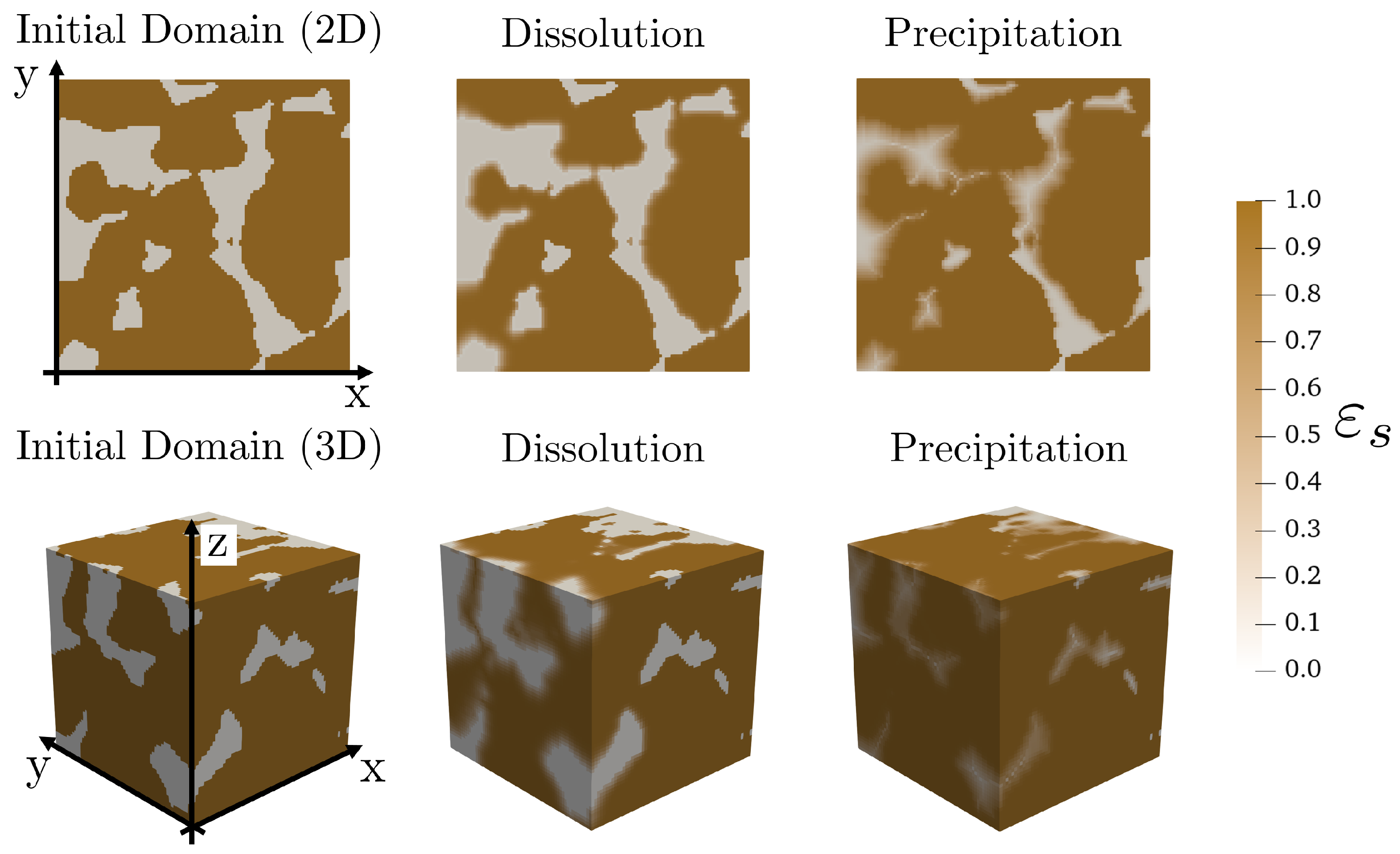
The initial distribution of the solid and fluid is determined by the imported sample (Figure 1); in this study, we assume ${\epsilon }_{\mathrm{s}}\in [0,0.95]$. For dissolution simulation, the equilibrium solid volume fraction is ${\epsilon }_{\mathrm{s},\mathrm{eq}}=0$, which leads to ${\epsilon }_{\mathrm{s}}>{\epsilon }_{\mathrm{s},\mathrm{eq}}$ and $r_{\mathrm{t}}<0$. For the precipitation scenario, ${\epsilon }_{\mathrm{s},\mathrm{eq}}$ is assigned a non-zero value, specifically ${\epsilon }_{\mathrm{s},\mathrm{eq}}=0.9$ in this study, and $r_{\mathrm{t}}>0$ when ${\epsilon }_{\mathrm{s}}<0.9$. Figure 1 shows how the pore geometry changes during dissolution or precipitation with an identical initial solid–fluid distribution. In the dissolution case, the solid volume fraction decreases as the reaction progresses and new pore connections form; in contrast, pore space shrinkage is observed in the precipitation simulation results. These changes in pore geometry lead to variations in flow properties, particularly the sample’s permeability. Furthermore, the intertwined flow, transport, and reaction processes result in an overall reaction rate that may deviate from that predicted by the homogeneous approximation. In this study, using the reactive transport model, we illustrate (1) how permeability changes dynamically during reaction and (2) how the overall reaction rate evolves in $\mathit{Pe}-\mathit{Da}$ space.

2.1. Geometric Properties

Porosity $\varphi$ [-] is computed by

$$\begin{array}{c}\hfill \varphi \left(t\right)={\displaystyle \frac{\int {\epsilon }_{\mathrm{f}}dV}{L^3}}.\end{array}$$

(24)

Additionally, we evaluate the specific surface area ${\mathsf{\Gamma }}_{\mathrm{r}}$ [m²·m⁻²] by selecting a contour of ${\epsilon }_{\mathrm{f}}=0.9$ at every time instance:

$$\begin{array}{c}\hfill {\mathsf{\Gamma }}_{\mathrm{r}}\left(t\right)={\displaystyle \frac{\int dA}{L^2}},\mathbf{x}\in \left\{(x,y,z)\right|{\epsilon }_{\mathrm{f}}=0.9\}.\end{array}$$

(25)

2.2. Permeability

In this study, we consider anisotropic permeability and retain the tensor form:

$$\begin{array}{c}\hfill {\mathbf{K}}^{\star }=\left[\begin{array}{ccc}{K}_{\mathrm{xx}}\hfill & K_{\mathrm{xy}}\hfill & K_{\mathrm{xz}}\hfill \\ K_{\mathrm{xy}}\hfill & K_{\mathrm{yy}}\hfill & K_{\mathrm{yz}}\hfill \\ K_{\mathrm{xz}}\hfill & K_{\mathrm{yz}}\hfill & K_{\mathrm{zz}}\hfill \end{array}\right],\end{array}$$

(26)

where ${\mathbf{K}}^{\star }$ denotes the permeability tensor, and $K_{ij},i,j=\{\mathrm{x},\mathrm{y},\mathrm{z}\}$ are the elements of the permeability tensor. We assume that the permeability tensor is symmetric, i.e., $K_{ij}=K_{ji}$. Computation of the permeability tensor follows the workflow introduced by Guibert et al. [36,37]. For a given pore geometry, three simulations with different velocity (or pressure) boundary conditions are needed; the velocity field of three simulations can be denoted as $\left[{\mathrm{u}}_{\mathrm{x}}^1,{\mathrm{u}}_{\mathrm{y}}^1,{\mathrm{u}}_{\mathrm{z}}^1\right]$, $\left[{\mathrm{u}}_{\mathrm{x}}^2,{\mathrm{u}}_{\mathrm{y}}^2,{\mathrm{u}}_{\mathrm{z}}^2\right]$, and $\left[{\mathrm{u}}_{\mathrm{x}}^3,{\mathrm{u}}_{\mathrm{y}}^3,{\mathrm{u}}_{\mathrm{z}}^3\right]$, and the corresponding pressure fields are ${\mathrm{p}}^1$, ${\mathrm{p}}^2$, and ${\mathrm{p}}^3$. The generalized Darcy’s law denotes

$$\begin{array}{c}\hfill 〈\mathbf{u}〉=-{\displaystyle \frac{{\mathbf{K}}^{\star }}{\mu }}·\overline{\nabla \mathrm{p}},\end{array}$$

(27)

where $〈·〉$ denotes the average over the entire domain:

$$\begin{array}{c}\hfill 〈·〉={\displaystyle \frac{1}{\left|\mathsf{\Omega }\right|}}\int dv,\end{array}$$

(28)

and $\overline{\nabla \mathrm{p}}$ is the effective pressure gradient, calculated by

$$\begin{array}{c}\hfill {\overline{\nabla \mathrm{p}}}_{\{\mathrm{x},\mathrm{y},\mathrm{z}\}}={\displaystyle \frac{{\overline{\mathrm{p}}}_{\{\mathrm{x},\mathrm{y},\mathrm{z}\}=\mathrm{L}}-{\overline{\mathrm{p}}}_{\{\mathrm{x},\mathrm{y},\mathrm{z}\}=0}}{L}},\end{array}$$

(29)

where ${\overline{\mathrm{p}}}_{\{\mathrm{x},\mathrm{y},\mathrm{z}\}=\mathrm{L}}$ is the average pressure evaluated at the outlet, and ${\overline{\mathrm{p}}}_{\{\mathrm{x},\mathrm{y},\mathrm{z}\}=0}$ is the average pressure evaluated at the inlet. The permeability tensor, then, is computed:

$${\mathbf{K}}^{\star }=\mu \left[\begin{array}{ccc}{\mathrm{u}}_{\mathrm{x}}^1\hfill & {\mathrm{u}}_{\mathrm{x}}^2\hfill & {\mathrm{u}}_{\mathrm{x}}^3\hfill \\ {\mathrm{u}}_{\mathrm{y}}^1\hfill & {\mathrm{u}}_{\mathrm{y}}^2\hfill & {\mathrm{u}}_{\mathrm{y}}^3\hfill \\ {\mathrm{u}}_{\mathrm{z}}^1\hfill & {\mathrm{u}}_{\mathrm{z}}^2\hfill & {\mathrm{u}}_{\mathrm{z}}^3\hfill \end{array}\right]{\left[\begin{array}{ccc}{\overline{\nabla {\mathrm{p}}^1}}_{\mathrm{x}}\hfill & {\overline{\nabla {\mathrm{p}}^2}}_{\mathrm{x}}\hfill & {\overline{\nabla {\mathrm{p}}^3}}_{\mathrm{x}}\hfill \\ {\overline{\nabla {\mathrm{p}}^1}}_{\mathrm{y}}\hfill & {\overline{\nabla {\mathrm{p}}^2}}_{\mathrm{y}}\hfill & {\overline{\nabla {\mathrm{p}}^3}}_{\mathrm{y}}\hfill \\ {\overline{\nabla {\mathrm{p}}^1}}_{\mathrm{z}}\hfill & {\overline{\nabla {\mathrm{p}}^2}}_{\mathrm{z}}\hfill & {\overline{\nabla {\mathrm{p}}^3}}_{\mathrm{z}}\hfill \end{array}\right]}^{-1},$$

(30)

where ${\left[·\right]}^{-1}$ denotes the inverse of the matrix. In this study, we focus on the major diagonal elements of the permeability tensor, i.e., $K_{\mathrm{xx}}$, $K_{\mathrm{yy}}$, and $K_{\mathrm{zz}}$. Normalized permeability elements are defined as

$$\begin{array}{c}\hfill K_{ii}^n={\displaystyle \frac{K_{ii}}{K_{\mathrm{xx}}+K_{\mathrm{yy}}+K_{\mathrm{zz}}}},ii=\{\mathrm{xx},\mathrm{yy},\mathrm{zz}\}\end{array}$$

(31)

2.3. Tortuosity

The tortuosity of the microstructure at every time instance is calculated based on the velocity field ([38,39]):

$$\begin{array}{c}\hfill {\tau }_i={\displaystyle \frac{〈\left|\mathbf{u}\right|〉}{〈{\mathrm{u}}_{\mathrm{i}}〉}}i=\{x,y,z\}\end{array}$$

(32)

where $\left|\mathbf{u}\right|$ is the velocity magnitude, and $u_i$ is the velocity component of i-direction. In our simulation, the solid-phase velocity is negligible due to the large flow resistance, such that $〈\left|\mathbf{u}\right|〉$ is dominated by pore-space velocity and physically meaningful.

2.4. Reaction Rate

Various methods have been proposed for effective reaction rate estimation [22,24,35,40]. In this study, we compute the effective reaction rate using the change of solid mass:

$$\begin{array}{c}\hfill {\mathrm{R}}^{\star }={\displaystyle \frac{\partial {\mathrm{M}}_{\mathrm{s}}}{\partial t}},\end{array}$$

(33)

where ${\mathrm{M}}_{\mathrm{s}}$ [kg] is the total solid mass:

$$\begin{array}{c}\hfill {\mathrm{M}}_{\mathrm{s}}={\rho }_{\mathrm{s}}\int {\epsilon }_{\mathrm{s}}dV.\end{array}$$

(34)

and the total mass change is computed:

$$\begin{array}{c}\hfill \mathsf{\Delta }{\mathrm{M}}_{\mathrm{s}}={\displaystyle \frac{|{\mathrm{M}}_{\mathrm{s}}\left(t_{\mathrm{end}}\right)-{\mathrm{M}}_{\mathrm{s}}(t=0)|}{M_{\mathrm{s},\max }}}\end{array}$$

(35)

where ${\mathrm{M}}_{\mathrm{s}}\left(t_{\mathrm{end}}\right)$ is the solid mass at the end of the simulation, ${\mathrm{M}}_{\mathrm{s}}(t=0)$ is the initial mass, and $M_{\mathrm{s},\max }=L^3{\rho }_{\mathrm{s}}$ is the maximum possible mass (when all the fluid is converted to solid).

3. Numerical Simulation

The solver is implemented in OpenFOAM, which is an open-source computational fluid dynamics (CFD) simulation platform. To solve the system of equations dynamically, the PIMPLE Algorithm is adopted. The PIMPLE algorithm combines PISO (Pressure Implicit with Splitting of Operator) and SIMPLE (Semi-Implicit Method for Pressure-Linked Equations). An adaptive time-stepping scheme was utilized, where the time step size was dynamically adjusted to maintain a local Courant number, ensuring numerical stability throughout the simulations. Equation (1) is used to obtain a momentum prediction, and the continuity (Equation (9)) is enforced by solving the pressure field. The solute transport (Equation (5)) and reaction (Equation (8)) are solved sequentially once the velocity and pressure fields converge. Details of the numerical implementation can be found in works by Soulaine et al. [27,28].

This study focuses on the interaction between flow and reaction—specifically, how dissolution/precipitation alters flow characteristics (e.g., permeability and tortuosity) and how flow influences reaction progression. Both two-dimensional (2D) and three-dimensional (3D) samples are used (

Table 1. Geometry used.

Geometry Label	Initial Porosity [-]	Dimension	Size [mm]
SG	0.73	2	2.0 × 2.0 × 0.01
SF	0.10
FP	0.39
S0	0.22	3	0.64 × 0.64 × 0.64
S1	0.16
S2	0.28
S3	0.20
S4	0.22

SG: Single solid grain; SF: Single fracture; FP: Fenny pack cross-section; S0: Barea Sandstone (B0 in [41]); S1–S4: Sandstone (S1–S4 in [41]).

). The size of the two-dimensional sample is 200 × 200 × 1 [pixels³], and 64 × 64 × 64 [pixels³] for the three-dimensional sample. The resolution is assumed to be 1 × 10⁻⁵ [m/pixel], and the corresponding domain sizes are 2.0 × 2.0 × 0.01 [m³] and 0.64 × 0.64 × 0.64 [m³]. Three 2D geometries are used: single grain (SG), fractured matrix (FM), and Fenny’s pack (FP). Six 3D samples are utilized in this study: Berea Sandstone (S0) and four sandstone samples (S1–S5) [41]. The parameters used in the simulations are ${\rho }_{\mathrm{f}}=1000$ kg·m⁻³, ${\rho }_{\mathrm{s}}=2710$ kg·m⁻³, $\mu =1\times {10}^{-6}$ kg·m⁻¹·s⁻¹, $R_{\mathrm{o}}=1\times {10}^7$ m⁻², $\mathrm{D}=9.31\times {10}^{-9}$ m²·s⁻¹, $\xi =1\times {10}^{-3}$.

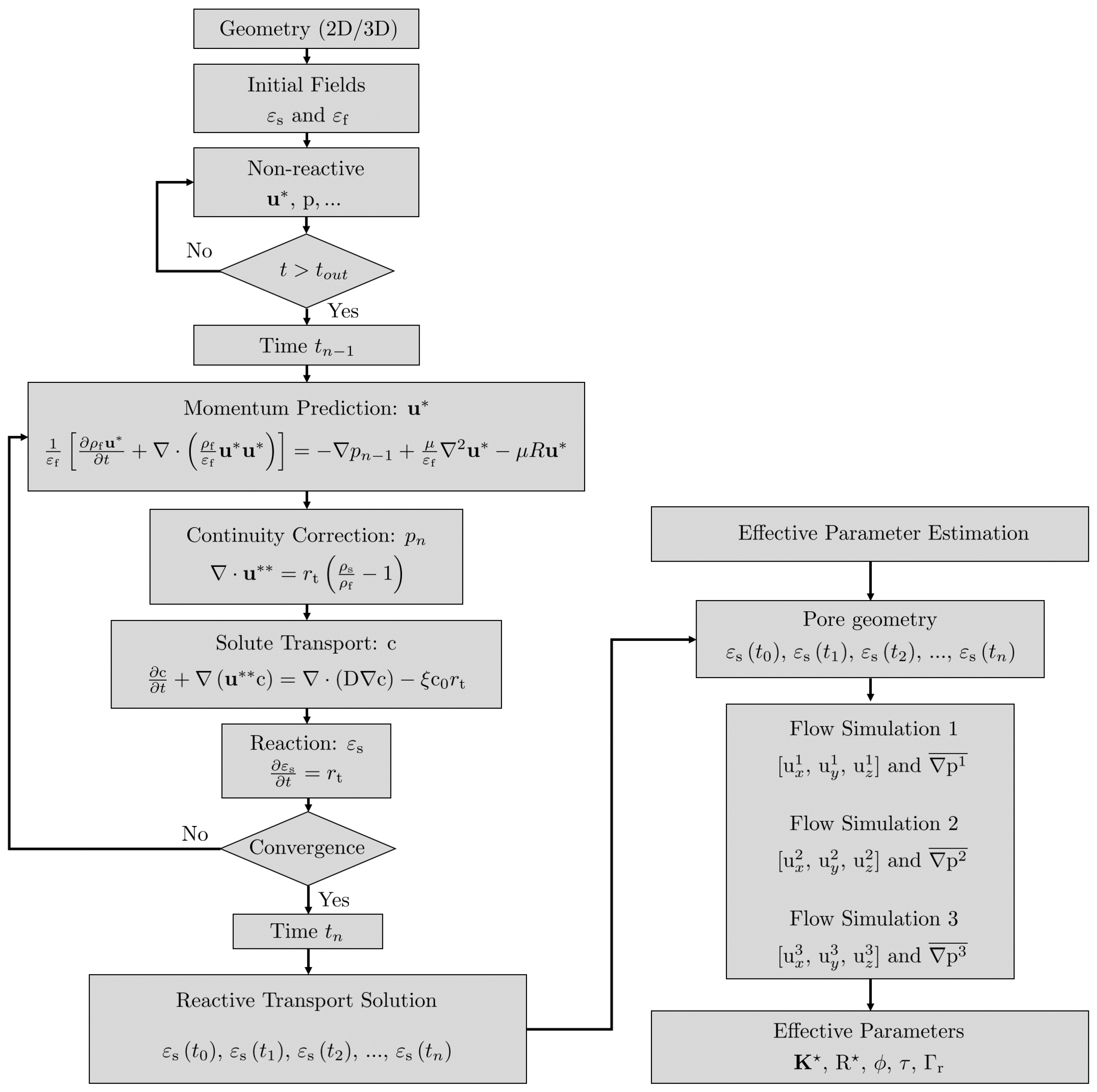
For each geometry, eight simulations are conducted: four dissolution cases and four precipitation ones. Every computation consists of three simulation stages (Figure 2): (1) non-reactive steady-state flow simulation, (2) reactive transport simulation, and (3) effective parameter estimation. The first stage establishes a steady-state flow field by setting the reaction rate to zero ($\alpha =0$) and the inlet concentration $c=0$, and the first stage lasts for one output time step (i.e., $t\in \left[0t_{out}\right]$). When $t>t_{out}$, i.e., the second stage, reactive fluid is injected from the inlet ($x=0$), and the reaction rate is non-zero, the pore geometry ${\epsilon }_{\mathrm{s}}(x,y,z,t)$ is stored at each output time instance ($t=n·t_{out},n=\{2,3,\dots \}$). The last stage is effective parameter estimation: the pore geometry at every time instance saved during the reactive simulation is imported, and then three simulations are conducted to compute the permeability tensor, tortuosity, porosity, and surface area. All simulations are performed using the Courant number $Co⩽0.2$ as the criterion; the total simulation time and output time step are listed in

Table 2. The simulation parameters.

Reaction Label	${\mathit{U}}_0$	$\mathit{\alpha }$	${\mathit{\epsilon }}_{\mathbf{s},\mathbf{eq}}$	3D Case $\mathit{Pe}$	3D Case ${\mathit{Da}}_{\mathit{I}}$
D01	1 × 10−3	1 × 10−1	0	68.7	0.064
D02	1 × 10−3	1 × 10−2	0	68.7	0.0064
D03	1 × 10−4	1 × 10−2	0	6.9	0.064
D04	1 × 10−4	1 × 10−3	0	6.9	0.0064
P01	1 × 10−3	1 × 10−1	9 × 10−1	68.7	0.064
P02	1 × 10−3	1 × 10−2	9 × 10−1	68.7	0.0064
P03	1 × 10−4	1 × 10−2	9 × 10−1	6.9	0.064
P04	1 × 10−4	1 × 10−3	9 × 10−1	6.9	0.0064

.

In this study, simulation is denoted by a combination of the geometry and the reaction label; for instance, dissolution simulation of the single-grain case with $U_0=1\times {10}^{-3}$, $\alpha =1\times {10}^{-1}$, and ${\epsilon }_{\mathrm{s},\mathrm{eq}}=0$ is denoted as SG-D01. All pre-processing, simulation, and post-processing are conducted in a Linux environment, Ubuntu 18.04. The geometry input file is either generated by a Python 3 script (for SG and SF) or input from digital rock (for FP [42], S0–S4 [41]). The Openfoam built-in function blockMesh and setFields are used to define the initial ${\epsilon }_{\mathrm{s}}$ and ${\epsilon }_{\mathrm{f}}$ fields. Post-processing integration or contour extraction is completed in Paraview.

4. Results

4.1. Validation

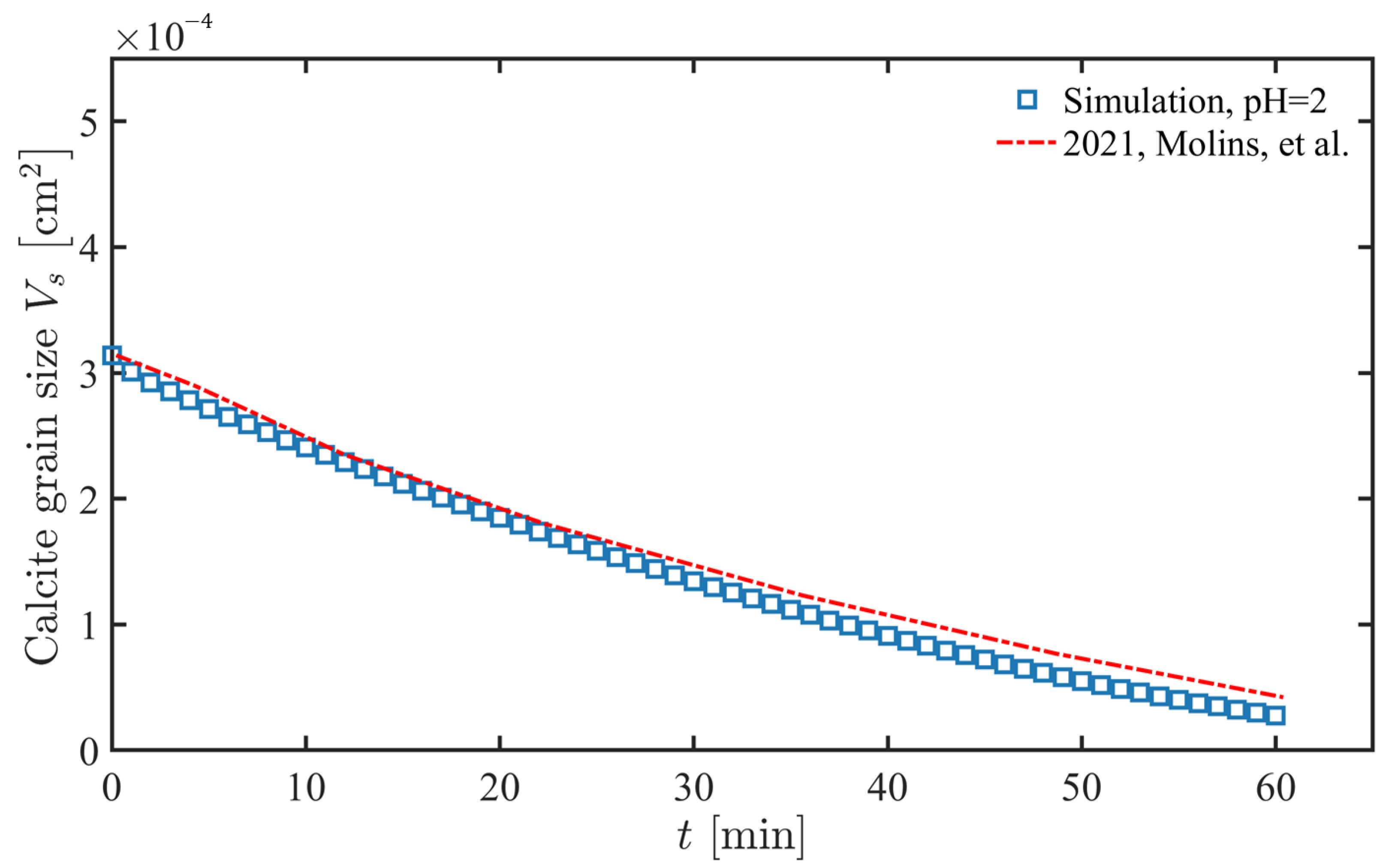
To validate the implementation, we employ the same case study shown in Figure 3, which was previously used by Molins et al. [25] to benchmark multiple reactive transport simulators. The system considers two minerals, calcite and dolomite, with calcite exhibiting a higher dissolution rate. The dissolution rate for calcite is adopted directly from Molins et al. [25], with all relevant parameters provided in

Table 3. Parameters used for the validation case.

Case	$\mathit{\alpha }$	${\mathit{c}}_0$	${\mathit{U}}_0$
Calcite, pH = 2	$0.89\times {10}^{-5}$	$1.0\times {10}^{-5}$	$1.2\times {10}^{-3}$

. The figure illustrates the evolution of the solid-grain volume over time, demonstrating that our simulation results are in good agreement with the experimental data.

4.2. Porosity and Surface Area

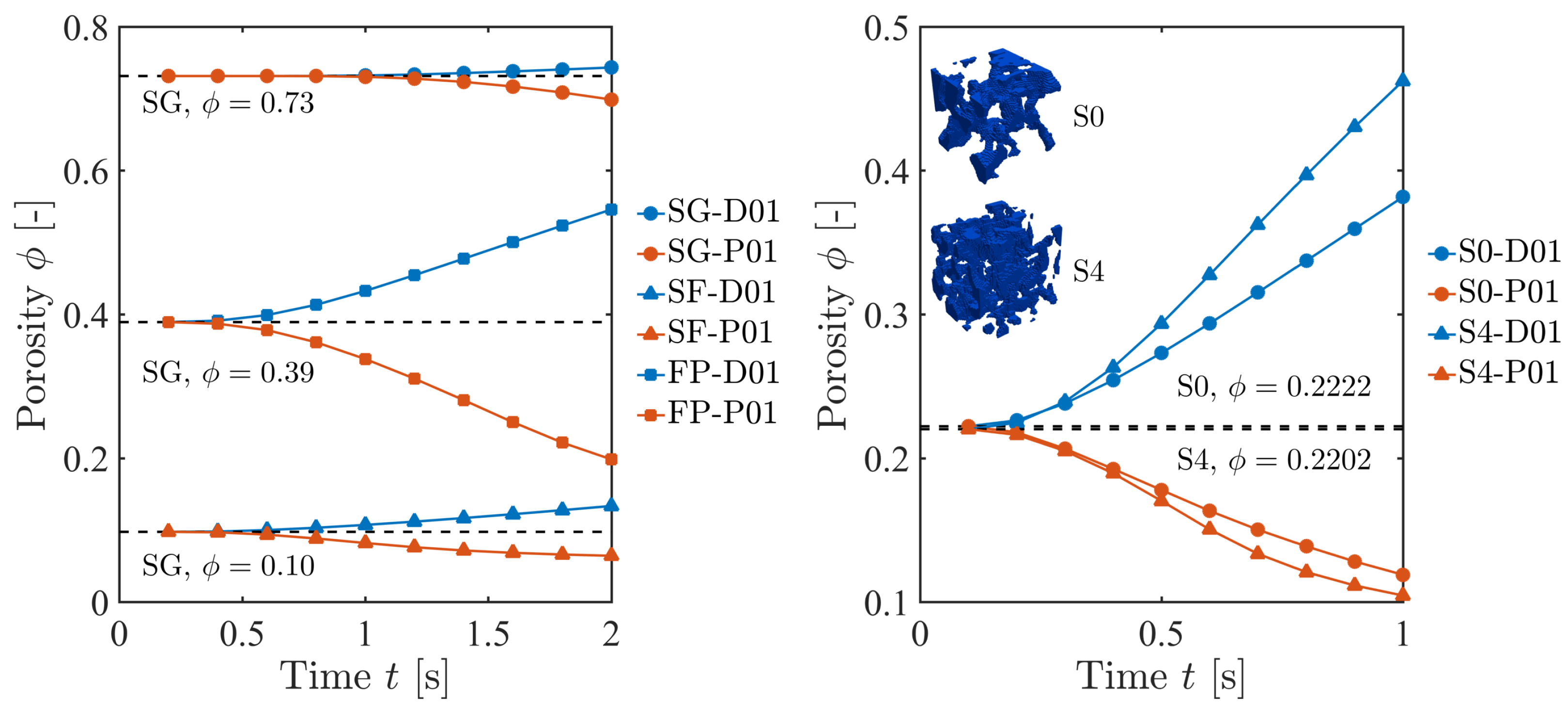
Porosity is computed at every output time ($t_{out}$) by Equation (24); the results of D01 and P01 are shown in Figure 4. The figure on the left includes 2D results, SG, SF, and FP; the figure on the right shows the results of two 3D geometries that have a similar initial porosity: S0 and S4. The simulations in this study consider a single, primary reactive species, enabling investigation of either dissolution or precipitation processes independently.

In Figure 4, the dashed black line illustrates the initial porosity, the blue curves are the results of dissolution simulation, and the red curves are the precipitation results. In the dissolution reaction, porosity increases at different rates, then decreases during precipitation, as expected. The change in porosity due to the reaction is not monotonically correlated with the initial porosity. For the 2D cases, the largest porosity is observed in the geometry (FP), which has the intermediate initial porosity. Similar initial porosity may result in a different final porosity, as shown in Figure 4—right. Such results show that reaction progression is strongly influenced by the pore geometry. Additionally, as observed in the pore geometry of S0 and S4 (Figure 4—right), narrower pore-throats and smaller pores correspond to more fluid–solid interfaces, which lead to a higher reaction rate and faster increase in porosity. As shown in the simulation, while porosity and permeability are bulk-averaged properties, reactivity is governed by the local pore-scale architecture. Specifically, we identify and analyze geometric features most responsible for the differential reaction rates. Well-connected pores ensure efficient delivery of reactants and removal of products. Samples with isolated pores or preferential flow channels exhibit a localized reaction. Also, narrow throats can create transport limitations, leading to a locally diffusion-controlled reaction, even in a sample with high overall permeability.

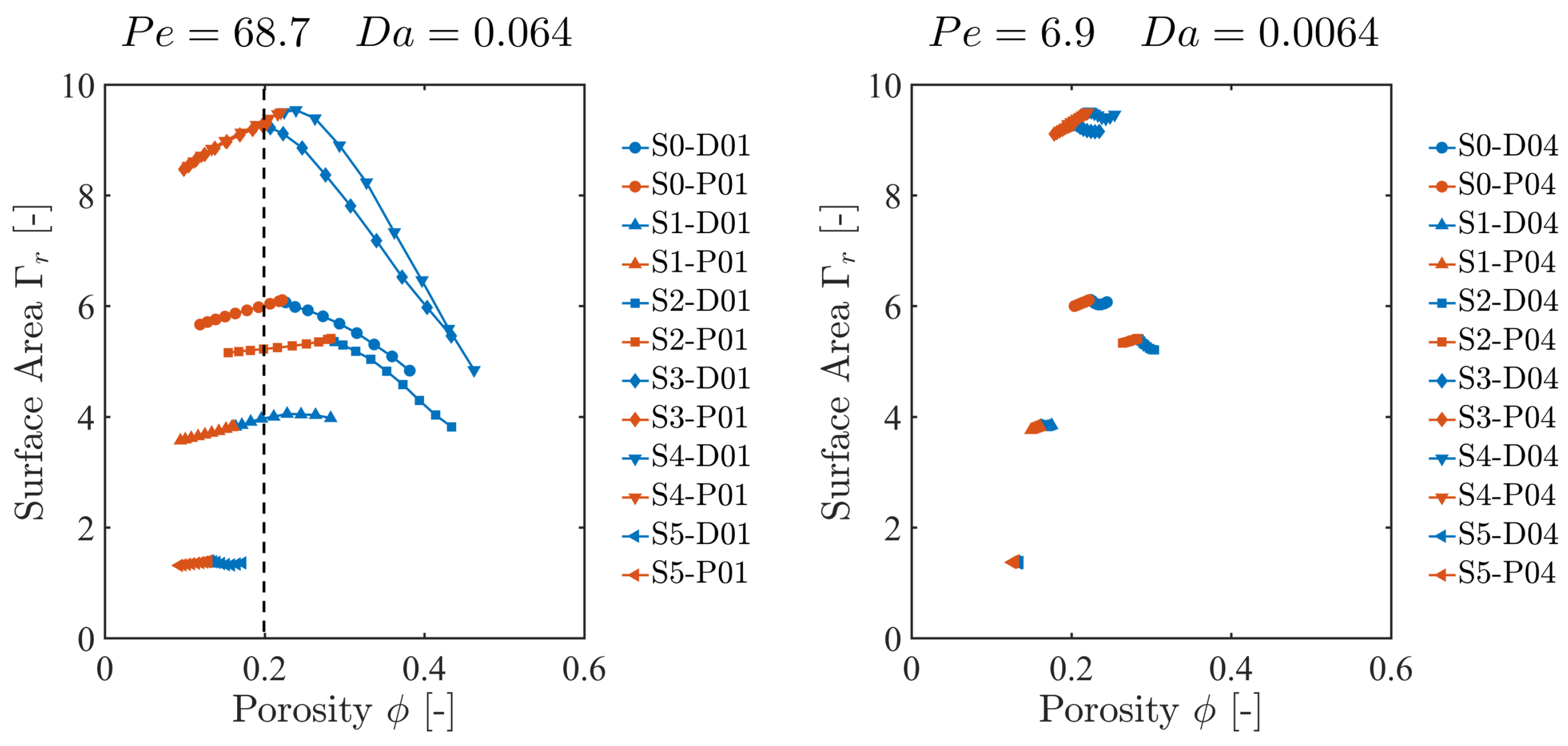
The ratio of surface area (or specific surface area) to porosity is frequently used to quantify reaction rates in reactive modeling. In existing studies [24,35], the $\varphi -{\mathsf{\Gamma }}_r$ relationship is obtained by assuming the reactive grains have a simple geometry, e.g., spheres or cubes. Figure 5 shows the results of all the 3D simulations with $\mathit{Pe}=68.7$ and ${\mathit{Da}}_I=0.064$ (left), and $\mathit{Pe}=6.9$ and ${\mathit{Da}}_I=0.064$ (right). Overall, when the initial porosity is larger than 0.2, ${\mathsf{\Gamma }}_r$ decreases linearly with the increase in porosity. In the high-$\mathit{Pe}$ and $\mathit{Da}$ scenario, when the initial porosity is larger than 0.2, i.e., S0 and S2–S4, the ${\mathsf{\Gamma }}_r-\varphi$ slope is large; when the initial porosity is less than 0.2, ${\mathsf{\Gamma }}_r-\varphi$ shows a smaller slope. When $\mathit{Pe}=6.9$ and ${\mathit{Da}}_I=0.064$, both $\varphi$ and ${\mathsf{\Gamma }}_r$ show a smaller change, and the surface area variation is not monotonic.

4.3. Permeability and Tortuosity

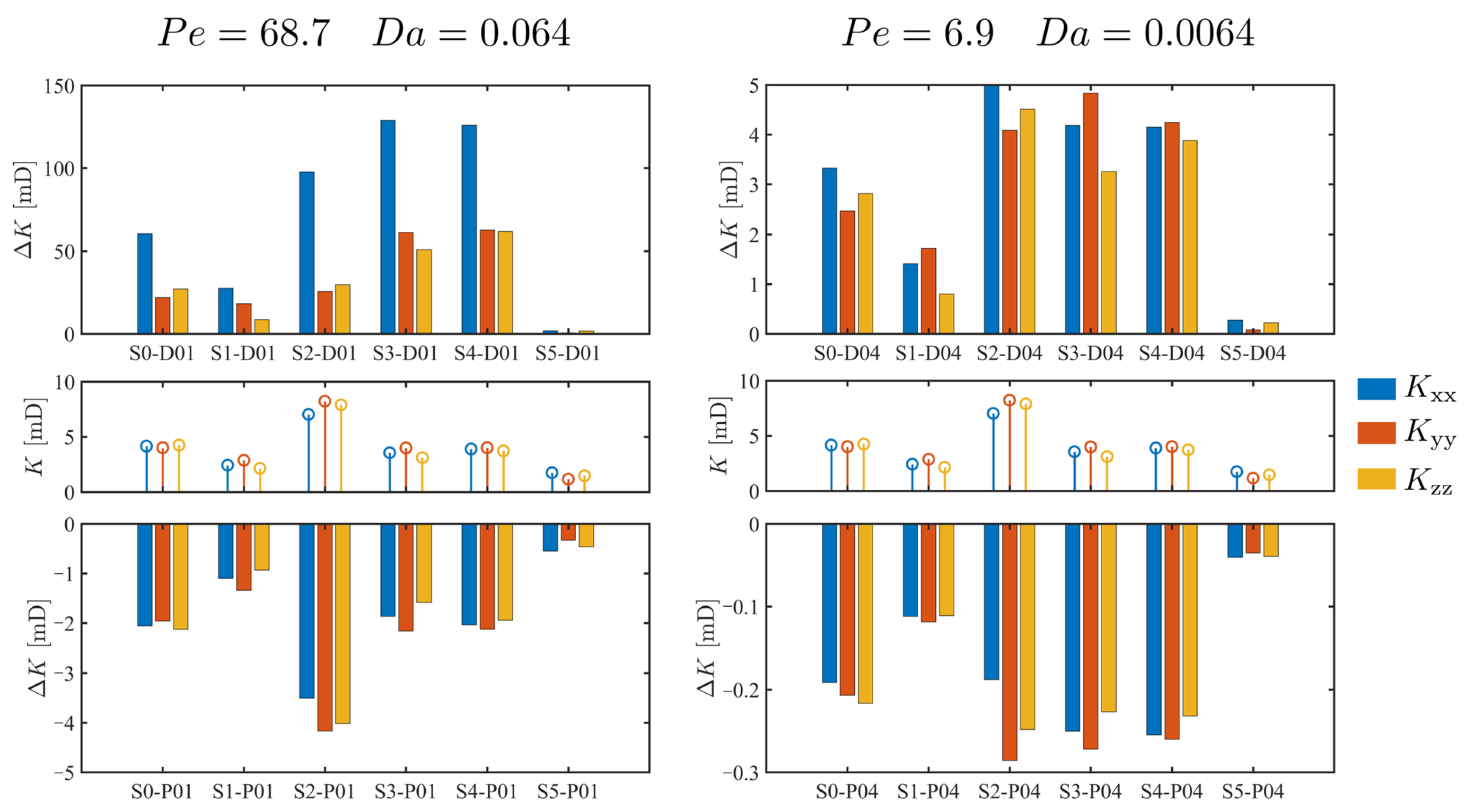
The impact of the reaction on the flow characteristics is quantified by tensorial permeability and tortuosity. Figure 6 shows the permeability results; the figure in the middle is the initial permeability of the digital sample, S0–S5. The top and bottom figures show the permeability changes due to dissolution and precipitation, respectively. The permeability change is calculated by

$$\begin{array}{c}\hfill \mathsf{\Delta }\mathrm{K}={\mathrm{K}}_{\mathrm{f}}-{\mathrm{K}}_{\mathrm{o}}.\end{array}$$

(36)

where ${\mathrm{K}}_{\mathrm{f}}$ is the permeability after dissolution or the precipitation reaction, and ${\mathrm{K}}_{\mathrm{o}}$ is the initial permeability. Figure 6 shows that the major components of the permeability tensor (${\mathrm{K}}_{\mathrm{xx}}$, ${\mathrm{K}}_{\mathrm{yy}}$, and ${\mathrm{K}}_{\mathrm{zz}}$) increase after dissolution, and they decrease after precipitation. The change in permeability in the $\mathit{Pe}=68.7$ and ${\mathit{Da}}_I=0.064$ case (D01 and P01) is ∼2 orders of magnitude larger compared to that of the $\mathit{Pe}=6.9$ and ${\mathit{Da}}_I=0.0064$ case (D04 and P04). Additionally, anisotropy is observed in the D01 case, where the x-direction permeability component ${\mathrm{K}}_{\mathrm{xx}}$ exhibits the largest increment. However, the D04 case presents a similar change across different geometries. The precipitation cases are more homogeneous.

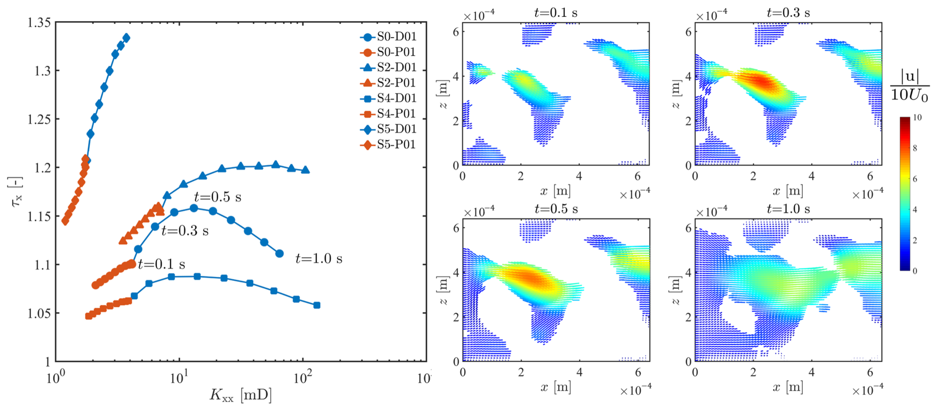
Anisotropy of the flow field is estimated by computing tortuosity (Equation (32)). We plot the x-direction tortuosity ${\tau }_{\mathrm{x}}$ and ${\mathrm{K}}_{\mathrm{xx}}$ in Figure 7-left. In Figure 7-right, we plot the velocity field of the S0 case at time t = 0.1, 0.3, 0.5, and 1.0 s. The selected cross-section is $\{\mathrm{x}\in [0,0.64\times {10}^{-3}]\}\cup \{\mathrm{y}\in [0.45\times {10}^{-3},0.48\times {10}^{-3}]\}\cup \{\mathrm{z}\in [0,0.64\times {10}^{-3}]\}$. In the initial stage of dissolution, tortuosity increases as the smaller pores are connected, as shown in Figure 7-right. Consequently, flow is influenced by the topology of the existing pores, leading to greater tortuosity. After most pores are connected ($t>0.5$ s for the S0-D01 case), dissolution begins to widen the existing fluid path, and the tortuous flow field becomes uni-directional.

4.4. Mass Change and Reaction Rate

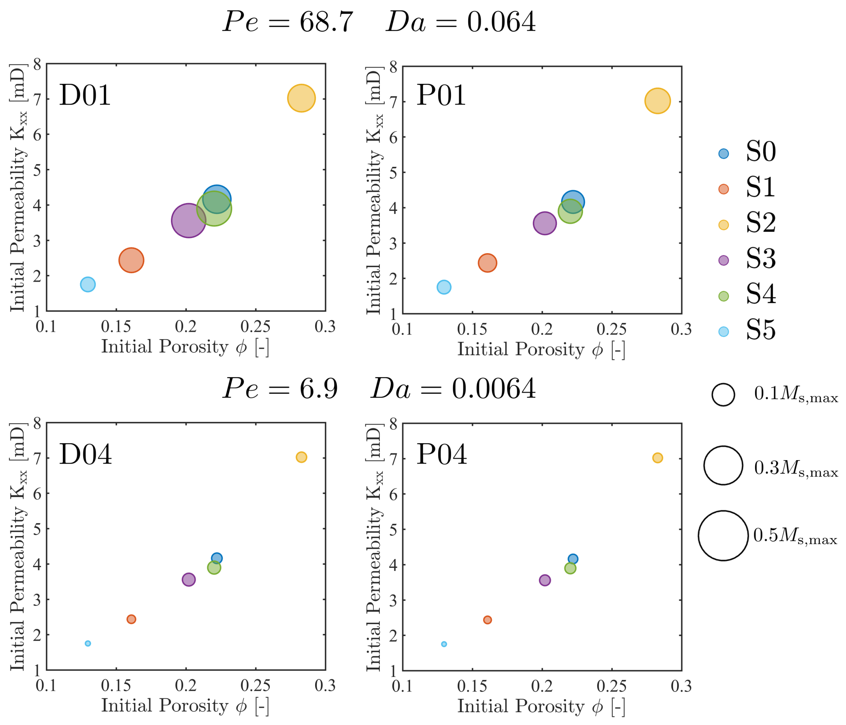
Reactivity assessment is crucial in many applications. In this study, we focus on two aspects: the total mass change ($\mathsf{\Delta }{\mathrm{M}}_{\mathrm{s}}$) and the reaction rate variation (${\mathrm{R}}^{\star }\left(t\right)$). In Figure 8, the size of the circle is determined by the $\mathsf{\Delta }{\mathrm{M}}_{\mathrm{s}}$ of the sample, the x-axis indicates the initial porosity, and the y-axis indicates the initial permeability. As shown in the $\mathit{Pe}=68.7$ and ${\mathit{Da}}_I=0.064$ results, the highest dissolved mass cases are S3 and S4, which are located at the intermediate initial porosity and permeability zone. Although S0 and S2 have a larger initial porosity and permeability, the dissolved mass is less than that of S3 and S4. The precipitation case shows less difference between cases. When the flow and reaction rate are lower (D04 and P04), the reacted mass is similar between cases. These results indicate that predicting reaction capacity solely from porosity and/or permeability may be inadequate in high-flow and reactive regimes.

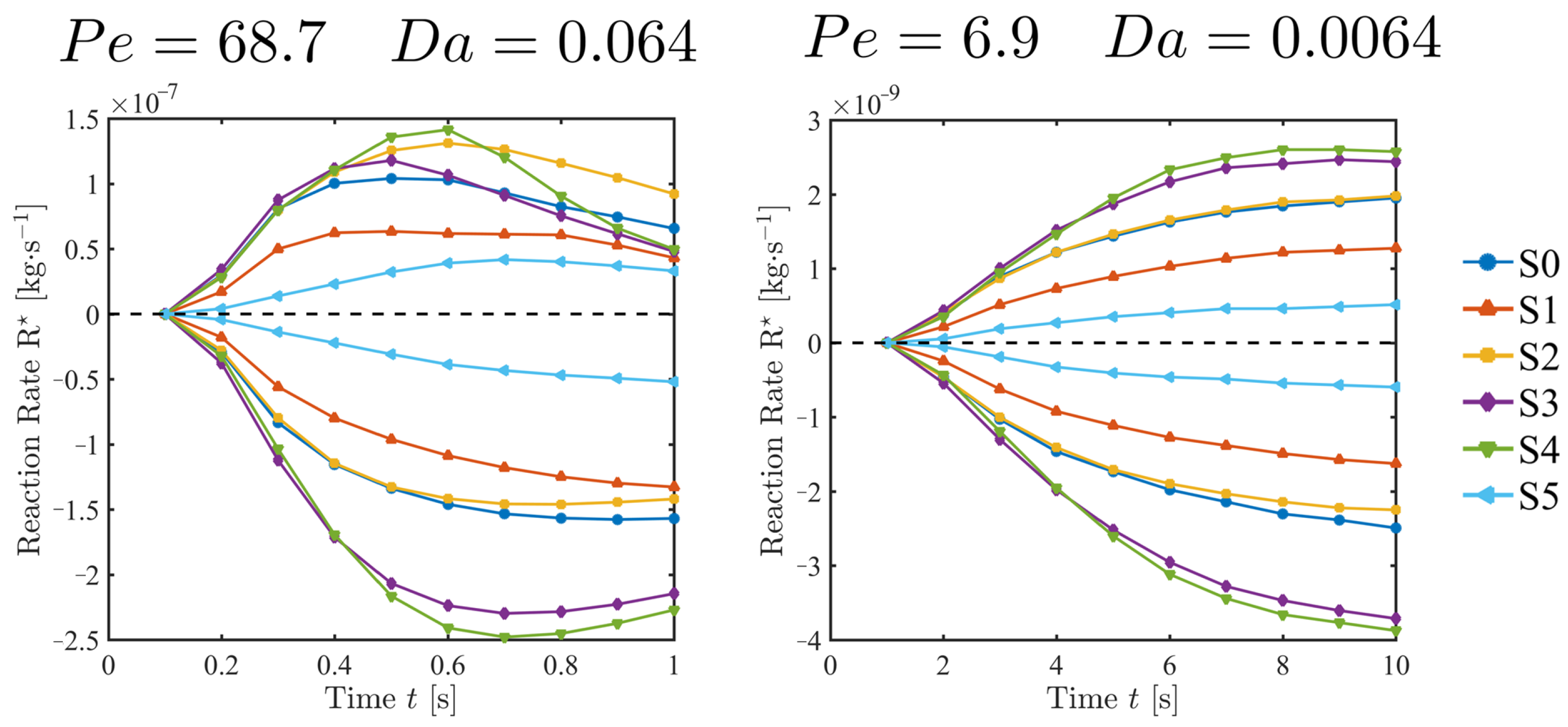
The reaction rate is plotted as a function of time in Figure 9. The dissolution rate is negative, and the precipitation rate is positive. For the high-flow rate and high-reactivity case, the reaction rate ramps up early; on the other hand, when $\mathit{Pe}$ and ${\mathit{Da}}_I$ are lower, the reaction increases slowly and reaches a plateau. These results indicate that the reaction rate is constant only when $\mathit{Pe}$ and ${\mathit{Da}}_I$ are small.

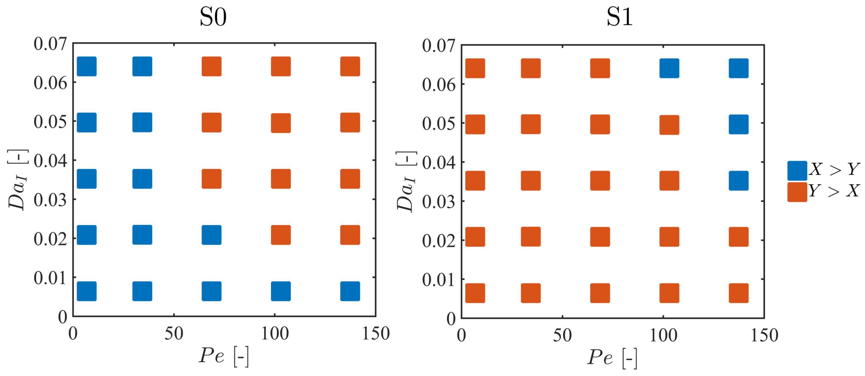
Moreover, one advantage of studying reactive transport using the numerical framework is the ability to run multiple tests on the same sample. Some subsurface formations exhibit strong anisotropy and directionality; when the flow direction changes, reactivity may change accordingly. To demonstrate, we conducted 25 simulations on one digital rock sample with flow injected along the x-direction and the same set of simulations on the same sample with flow injected from the y-direction. We selected S0 and S1, assuming each undergoes a dissolution reaction for $t=1$ [s] with 25 combinations of $\mathit{Pe}$ and ${\mathit{Da}}_I$. The results are shown in Figure 10. We compare the total mass reacted ($\mathsf{\Delta }{\mathrm{M}}_{\mathrm{s}}$) by dissolution. If x-direction injection consumes more mass, the dot is blue, and if more mass is reacted when injecting from y, the marker is red. We see that both cases exhibit an alternation as $\mathit{Pe}$ and ${\mathit{Da}}_I$ increase, indicating an optimal reactive transport regime that is anisotropic. Also, the results suggest that the new framework can be used to identify the maximum reactivity condition of a given digital rock sample.

5. Conclusions

In this study, we adopted the MCA and implemented a reactive-transport solver in the OpenFOAM environment. We also developed a numerical workflow that computes effective parameters for each time instance output by the reactive solver. Additionally, a pre-processing algorithm was constructed to import digital rock samples. The newly developed framework fulfills the following tasks:

• Performing numerical dissolution/precipitation simulation on digital samples and predicting geometry evolution.
• Evaluating the flow and transport property as the reaction progresses. The properties are the porosity, surface area, permeability tensor, tortuosity, mass, and reaction rate.
• Assessing flow anisotropy and heterogeneity induced by reaction.
• Estimating the mass change and transient reaction rate of a given sample under certain flow and reaction conditions.

The results show that the reaction has a significant impact on the pore geometry and the effective parameters, and that the initial geometry significantly alters the reaction progression. Specifically, the reaction rate is not a monotonic function of the porosity, nor of the permeability. The temporal variation of the reaction rate is also complex. When the transport process is more advective ($\mathit{Pe}\ll 1$), the reaction rate varies; when $\mathit{Pe}\sim 1$, the reaction rate plateaus after a certain time. The result indicates that approximating the reaction rate as a constant may lead to deviation when the flow effect is strong. As shown in the permeability tensor results for the dissolution scenario, when the flow rate is high, the permeability increment is anisotropic. The precipitation shows a more homogeneous change of the permeability tensor elements. Analysis of tortuosity shows that, at the initial stage of dissolution, pores are connected, and flow paths become increasingly tortuous. As dissolution progresses, pores widen, and the flow becomes more unidirectional. The main limitations are as follows: (1) The current model uses a single-reaction system. Real-world applications, such as CO₂ mineralization, involve complex multi-mineral assemblages and multi-component chemistry. (2) The framework provides excellent pore-scale insights but requires upscaling to inform field-scale models.

Some future developments are being considered: (1) extending the reactive solver to multi-solute and multi-mineral systems, combined with compositional analysis (e.g., Energy-Dispersive Spectroscopy, EDS) of samples and prediction of how minerals change when in contact with reactive fluids; (2) performing an optimization study on applications such as CO₂ storage via mineralization or reactive fracturing for shale formation; (3) implementing effective parameter-estimation modules with different physics, e.g., mechanical moduli estimation after a reaction. Beyond the geochemical systems studied here, the principles governing reactions in porous media may extend to other natural systems. Bio-material (e.g., bones) is one such example. Exploring the model’s applicability to bone-related processes, such as osteoporosis, is a compelling but distinct direction for future study. Additionally, this framework is modular and can be extended to incorporate chemo-mechanical coupling by integrating MCA with geomechanical models (e.g., the Discrete Element Method, DEM) or poromechanics equations—an important future direction to enhance applicability to high-stress subsurface systems (e.g., CO₂ caprock integrity under in situ stress). In such cases, permeability evolution would further depend on stress-induced changes in pore/aperture geometry, and the current toolbox provides a baseline for comparing geometry-driven vs. stress-driven alterations in hydraulic properties.

References

1. Goldberg, D.S.; Takahashi, T.; Slagle, A.L. Carbon dioxide sequestration in deep-sea basalt. Proc. Natl. Acad. Sci. USA 2008, 105, 9920–9925. [Google Scholar] [CrossRef] [Scilit] [PubMed]
2. Gislason, S.R.; Oelkers, E.H. Carbon storage in basalt. Science 2014, 344, 373–374. [Google Scholar] [CrossRef] [Scilit] [PubMed]
3. Wu, W.; Sharma, M.M. Acid fracturing in shales: Effect of dilute acid on properties and pore structure of shale. SPE Prod. Oper. 2017, 32, 51–63. [Google Scholar] [CrossRef] [Scilit]
4. Grieser, W.V.; Wheaton, W.E.; Magness, W.D.; Blauch, M.E.; Loghry, R. Surface Reactive Fluid’s Effect on Shale. In Proceedings of the Production and Operations Symposium, Oklahoma City, OK, USA, 31 March 31–3 April 2007. [Google Scholar] [CrossRef]
5. Powell, R.M.; Puls, R.W.; Hightower, S.K.; Sabatini, D.A. Coupled iron corrosion and chromate reduction: Mechanisms for subsurface remediation. Environ. Sci. Technol. 1995, 29, 1913–1922. [Google Scholar] [CrossRef] [Scilit]
6. Vidonish, J.E.; Alvarez, P.J.; Zygourakis, K. Pyrolytic remediation of oil-contaminated soils: Reaction mechanisms, soil changes, and implications for treated soil fertility. Ind. Eng. Chem. Res. 2018, 57, 3489–3500. [Google Scholar] [CrossRef] [Scilit]
7. Cundy, A.B.; Hopkinson, L.; Whitby, R.L. Use of iron-based technologies in contaminated land and groundwater remediation: A review. Sci. Total Environ. 2008, 400, 42–51. [Google Scholar] [CrossRef] [Scilit]
8. Ginn, T.R.; Wood, B.D.; Nelson, K.E.; Scheibe, T.D.; Murphy, E.M.; Clement, T.P. Processes in microbial transport in the natural subsurface. Adv. Water Resour. 2002, 25, 1017–1042. [Google Scholar] [CrossRef] [Scilit]
9. Yan, Z.; Liu, C.; Liu, Y.; Bailey, V.L. Multiscale investigation on biofilm distribution and its impact on macroscopic biogeochemical reaction rates. Water Resour. Res. 2017, 53, 8698–8714. [Google Scholar] [CrossRef] [Scilit]
10. Moldoveanu, G.A.; Papangelakis, V.G. Recovery of rare earth elements adsorbed on clay minerals: I. Desorption mechanism. Hydrometallurgy 2012, 117, 71–78. [Google Scholar] [CrossRef] [Scilit]
11. Moldoveanu, G.A.; Papangelakis, V.G. Recovery of rare earth elements adsorbed on clay minerals: II. Leaching with ammonium sulfate. Hydrometallurgy 2013, 131, 158–166. [Google Scholar] [CrossRef] [Scilit]
12. Jun, T.; Jingqun, Y.; Kaihong, C.; Guohua, R.; Mintao, J.; Ruan, C. Optimisation of mass transfer in column elution of rare earths from low grade weathered crust elution-deposited rare earth ore. Hydrometallurgy 2010, 103, 211–214. [Google Scholar] [CrossRef] [Scilit]
13. Okamoto, I.; Li, X.; Ohsumi, T. Effect of supercritical CO2 as the organic solvent on cap rock sealing performance for underground storage. Energy 2005, 30, 2344–2351. [Google Scholar] [CrossRef] [Scilit]
14. Deng, H.; Fitts, J.P.; Tappero, R.V.; Kim, J.J.; Peters, C.A. Acid erosion of carbonate fractures and accessibility of arsenic-bearing minerals: In Operando synchrotron-based microfluidic experiment. Environ. Sci. Technol. 2020, 54, 12502–12510. [Google Scholar] [CrossRef] [Scilit] [PubMed]
15. Vorhies, J.S.; Gaines, R.R. Microbial dissolution of clay minerals as a source of iron and silica in marine sediments. Nat. Geosci. 2009, 2, 221–225. [Google Scholar] [CrossRef] [Scilit]
16. Al-Khulaifi, Y.; Lin, Q.; Blunt, M.J.; Bijeljic, B. Reaction rates in chemically heterogeneous rock: Coupled impact of structure and flow properties studied by X-ray microtomography. Environ. Sci. Technol. 2017, 51, 4108–4116. [Google Scholar] [CrossRef] [Scilit]
17. Li, L.; Peters, C.A.; Celia, M.A. Effects of mineral spatial distribution on reaction rates in porous media. Water Resour. Res. 2007, 43. [Google Scholar] [CrossRef] [Scilit]
18. Song, W.; Ogunbanwo, F.; Steinsbø, M.; Fernø, M.A.; Kovscek, A.R. Mechanisms of multiphase reactive flow using biogenically calcite-functionalized micromodels. Lab Chip 2018, 18, 3881–3891. [Google Scholar] [CrossRef] [Scilit]
19. Sun, H.; Yao, J.; Cao, Y.C.; Fan, D.Y.; Zhang, L. Characterization of gas transport behaviors in shale gas and tight gas reservoirs by digital rock analysis. Int. J. Heat Mass Trans. 2017, 104, 227–239. [Google Scholar] [CrossRef] [Scilit]
20. Sun, H.; Belhaj, H.; Tao, G.; Vega, S.; Liu, L. Rock properties evaluation for carbonate reservoir characterization with multi-scale digital rock images. J. Petrol. Sci. Eng. 2019, 175, 654–664. [Google Scholar] [CrossRef] [Scilit]
21. Sadeghnejad, S.; Enzmann, F.; Kersten, M. Digital rock physics, chemistry, and biology: Challenges and prospects of pore-scale modelling approach. Appl. Geochem. 2021, 131, 105028. [Google Scholar] [CrossRef] [Scilit]
22. Steefel, C.I.; Maher, K. Fluid-rock interaction: A reactive transport approach. Rev. Minearal Geochem. 2009, 70, 485–532. [Google Scholar] [CrossRef] [Scilit]
23. Steefel, C.I.; Molins, S.; Trebotich, D. Pore Scale Processes Associated with Subsurface CO2 Injection and Sequestration. Rev. Minearal Geochem. 2013, 77, 259–303. [Google Scholar] [CrossRef] [Scilit]
24. Beckingham, L.E.; Mitnick, E.H.; Steefel, C.I.; Zhang, S.; Voltolini, M.; Swift, A.M.; Yang, L.; Cole, D.R.; Sheets, J.M.; Ajo-Franklin, J.B.; et al. Evaluation of mineral reactive surface area estimates for prediction of reactivity of a multi-mineral sediment. Geochim. Cosmochim. Acta 2016, 188, 310–329. [Google Scholar] [CrossRef] [Scilit]
25. Molins, S.; Soulaine, C.; Prasianakis, N.I.; Abbasi, A.; Poncet, P.; Ladd, A.J.; Starchenko, V.; Roman, S.; Trebotich, D.; Tchelepi, H.A.; et al. Simulation of mineral dissolution at the pore scale with evolving fluid-solid interfaces: Review of approaches and benchmark problem set. Computat. Geosci. 2021, 25, 1285–1318. [Google Scholar] [CrossRef] [Scilit]
26. Steefel, C.I.; Beckingham, L.E.; Landrot, G. Micro-continuum approaches for modeling pore-scale geochemical processes. Rev. Minearal Geochem. 2015, 80, 217–246. [Google Scholar] [CrossRef] [Scilit]
27. Soulaine, C.; Tchelepi, H.A. Micro-continuum approach for pore-scale simulation of subsurface processes. Transp. Porous Med. 2016, 113, 431–456. [Google Scholar] [CrossRef] [Scilit]
28. Soulaine, C.; Roman, S.; Kovscek, A.; Tchelepi, H.A. Mineral dissolution and wormholing from a pore-scale perspective. J. Fluid Mech. 2017, 827, 457–483. [Google Scholar] [CrossRef] [Scilit]
29. Soulaine, C.; Roman, S.; Kovscek, A.; Tchelepi, H.A. Pore-scale modelling of multiphase reactive flow: Application to mineral dissolution with production of CO2. J. Fluid Mech. 2018, 855, 616–645. [Google Scholar] [CrossRef] [Scilit]
30. Liu, Y.; Min, J.; Zhang, X. A novel micro-continuum lattice Boltzmann approach for multiscale modeling immiscible two-phase flow in porous media. Phys. Fluids 2024, 36, 083345. [Google Scholar] [CrossRef] [Scilit]
31. Fogouang, L.M.; André, L.; Soulaine, C. Particulate transport in porous media at pore-scale. Part 1: Unresolved-resolved four-way coupling CFD-DEM. J. Comput. Phys. 2025, 521, 113540. [Google Scholar] [CrossRef] [Scilit]
32. Soulaine, C. Micro-continuum modeling: An hybrid-scale approach for solving coupled processes in porous media. Water Resour. Res. 2024, 60, e2023WR035908. [Google Scholar] [CrossRef] [Scilit]
33. Ellis, B.R.; Fitts, J.P.; Bromhal, G.S.; McIntyre, D.L.; Tappero, R.; Peters, C.A. Dissolution-driven permeability reduction of a fractured carbonate caprock. Environ. Eng. Sci. 2013, 30, 187–193. [Google Scholar] [CrossRef] [Scilit] [PubMed]
34. Noiriel, C.; Steefel, C.I.; Yang, L.; Ajo-Franklin, J. Upscaling calcium carbonate precipitation rates from pore to continuum scale. Chem. Geol. 2012, 318, 60–74. [Google Scholar] [CrossRef] [Scilit]
35. Qin, F.; Beckingham, L.E. The impact of mineral reactive surface area variation on simulated mineral reactions and reaction rates. Appl. Geochem. 2021, 124, 104852. [Google Scholar] [CrossRef] [Scilit]
36. Guibert, R.; Nazarova, M.; Horgue, P.; Hamon, G.; Creux, P.; Debenest, G. Computational permeability determination from pore-scale imaging: Sample size, mesh and method sensitivities. Transp. Porous Med. 2015, 107, 641–656. [Google Scholar] [CrossRef] [Scilit]
37. Guibert, R.; Horgue, P.; Debenest, G.; Quintard, M. A comparison of various methods for the numerical evaluation of porous media permeability tensors from pore-scale geometry. Math. Geosci. 2016, 48, 329–347. [Google Scholar] [CrossRef] [Scilit]
38. Duda, A.; Koza, Z.; Matyka, M. Hydraulic tortuosity in arbitrary porous media flow. Phys. Rev. E 2011, 84, 036319. [Google Scholar] [CrossRef] [Scilit]
39. Miller, K.; Vanorio, T.; Keehm, Y. Evolution of permeability and microstructure of tight carbonates due to numerical simulation of calcite dissolution. J. Geophys. Res. Solid Earth 2017, 122, 4460–4474. [Google Scholar] [CrossRef] [Scilit]
40. Nogues, J.P.; Fitts, J.P.; Celia, M.A.; Peters, C.A. Permeability evolution due to dissolution and precipitation of carbonates using reactive transport modeling in pore networks. Water Resour. Res. 2013, 49, 6006–6021. [Google Scholar] [CrossRef] [Scilit]
41. Dong, H.; Blunt, M.J. Pore-network extraction from micro-computerized-tomography images. Phys. Rev. E 2009, 80, 036307. [Google Scholar] [CrossRef] [Scilit]
42. Santos, J.E.; Yin, Y.; Prodanovic, M.; Gigliotti, A.; Lubbers, N.; Khan, H. 3D Collection of Binary Images. 2021. Available online: http://www.digitalrocksportal.org/projects/374 (accessed on 15 January 2026).
Figure 1. Examples of two-dimensional and three-dimensional domains before and after reaction.
Applsci 16 01287 g001
Figure 2. Flow chart of the numerical framework implemented in this study.
Applsci 16 01287 g002
Figure 3. The blue square marker represents the volume of calcite grains as a function of time, and the dashed red line is the validation case presented in the literature [25].
Applsci 16 01287 g003
Figure 4. (Left): Porosity change during reaction in 2D cases: SG, SF, and FP. (Right): Porosity change during reaction in 3D cases: S0 and S4. The dashed black line indicates the initial porosity of each case, the blue curve indicates the dissolution result (D01), and the red curve illustrates the result of the precipitation (P01). The black dashed line indicates the initial porosity of each case.
Applsci 16 01287 g004
Figure 5. (Left): Porosity–surface area change during reaction in 3D cases when Pe = 68.7 and Da I = 0.064 . (Right): Porosity–surface area change during reaction in 3D cases when Pe = 6.9 and Da I = 0.0064 . The blue curve indicates the dissolution result (D01), and the red curve is the result of precipitation (P01). The black dashed line indicates the initial porosity of each case.
Applsci 16 01287 g005
Figure 6. (Top): The permeability change in the dissolution case. (Middle): The initial permeability of each case. (Bottom): The permeability change in the precipitation case. Blue color indicates the permeability of the x-direction, red indicates the y-direction result, and yellow indicates the z-direction. Figures on the (left) are Pe = 68.7 and Da I = 0.64 (left), and the results of Pe = 6.9 and Da I = 0.0064 are shown on the (right).
Applsci 16 01287 g006
Figure 7. (Left): The x-direction tortuosity and permeability ( τ x - K xx ) of different samples; the blue branch illustrates the dissolution, and the red branch indicates the results of precipitation. (Right): The velocity field of the S0 case at time t = 0.1, 0.3, 0.5, and 1.0 s. The selected cross-section is { x [ 0 , 0.64 × 10 3 ] } { y [ 0.45 × 10 3 , 0.48 × 10 3 ] } { z [ 0 , 0.64 × 10 3 ] } . The segments are velocity vectors, and the color represents the velocity magnitude normalized by 10 U 0 .
Applsci 16 01287 g007
Figure 8. The mass change of S0–S5. The x-axis indicates the initial porosity, and the y-axis indicates the initial permeability K xx . (Top): The simulation results of Pe = 68.7 and Da I = 0.064 . (Bottom): The simulation results of Pe = 6.9 and Da I = 0.0064 .
Applsci 16 01287 g008
Figure 9. The reaction rate variation as a function of time.
Applsci 16 01287 g009
Figure 10. A comparison of the reacted mass with different injection directions and reactive transport conditions. If more mass is reacted when injecting from the x-direction, the marker is blue, and when the y-direction injection reacts with more mass, the marker is red.
Applsci 16 01287 g010