Article

Power Grid Electrification Through Grid Extension and Microgrid Deployment: A Case Study of the Navajo Nation


1
Advanced Energy Systems Program, Colorado School of Mines, Golden, CO 80401, USA
2
Electrical and Electronic Engineering Department, Jazan University, Jazan 45142, Saudi Arabia
3
Department of Civil, Environmental, and Geodetic Engineering, The Ohio State University, Columbus, OH 43210, USA
4
School of Engineering, Math, and Technology, Navajo Technical University, Crownpoint, NM 87313, USA
5
Electrical Engineering Department, Colorado School of Mines, Golden, CO 80401, USA
*
Author to whom correspondence should be addressed.
Appl. Sci. 2026, 16(3), 1227; https://doi.org/10.3390/app16031227
Submission received: 6 December 2025 / Revised: 20 January 2026 / Accepted: 20 January 2026 / Published: 25 January 2026
(This article belongs to the Special Issue Recent Advances in Smart Microgrids)

Abstract

Ensuring affordable and reliable electricity access to areas with low population density is challenging, as network sparsity and lower connectivity rates can make it nearly impossible for electric utilities to cover the cost of interconnection without raising electricity tariffs. Utility providers that consider extending their networks to remote households must balance multiple and often conflicting objectives, including investment cost, grid resilience, geographical coverage, and environmental impacts. In this paper, a multi-objective decision-making framework is proposed for the electrification of rural households, considering traditional distribution network extension as well as microgrid deployment. In order to condense a wide range of spatial inputs into a tractable problem, a multi-criteria decision-making approach is adopted to identify and rank candidate sites for microgrid deployment that offer superior performance over a variety of technical, environmental, and economic criteria. A novel optimization model is then proposed using multi-objective Chebyshev goal programming, in which project costs, environmental impacts, and energy justice criteria are jointly optimized. The applicability of this framework is demonstrated through a case study of the Shiprock region within the Navajo Nation. The results indicate that the proposed methodology provides a balanced trade-off among conflicting objectives and identifies a priority order of loads to energize first under marginally increasing budgets.

1. Introduction

Access to reliable and affordable electricity is one of the most important requirements for ensuring health, education, and economic development. However, in 2022, around 685 million people worldwide were without electricity. While there have been many electrification projects worldwide, in some areas, population growth may outpace these efforts. Most unelectrified households are located in rural and remote areas where population density is low, terrain makes access and construction difficult, and the cost of extending the existing grid is extremely high [1]. A global assessment shows that almost half of new electricity connections needed by 2030 will have to come from off-grid and mini-grid systems because conventional grid expansion may not be feasible or cost-effective [2]. These conditions have shifted interest toward microgrids as a practical solution for providing electricity to remote and disadvantaged communities.
A microgrid is a localized system that integrates distributed generation, energy storage, and controllable loads that can either draw energy from the main grid or operate as an islanded system [3]. Microgrids are suitable for remote regions because they can use locally available renewable energy resources such as solar and wind to provide reliable electricity at lower costs compared to long-distance line extensions [4]. Microgrids are also important for improving resilience. Climate change has increased the frequency and severity of storms, wildfires, and other hazardous events, which has highlighted vulnerabilities in centralized power systems [5,6]. In 2020, for instance, the average electricity customer in the United States experienced more than eight hours of power interruption, the highest recorded value [7]. Rural areas often experience longer outages because the distribution network is more widespread, with longer feeders, and has limited redundancy [8]. On the other hand, microgrids can isolate themselves from the main grid during disturbances and continue to supply critical loads, making them an effective tool for enhancing reliability and resilience [8,9,10].
The Navajo Nation exemplifies the above challenges and opportunities associated with remote electrification. It covers almost 27,000 square miles (70,000 square km) across the states of Arizona, New Mexico, and Utah and is the largest Indigenous reservation in the United States [8]. Despite its size, many households still do not have electricity. It is estimated that around 14,000 homes, which represents roughly 21% of all households within the reservation, remain unelectrified, which is the largest concentration of unelectrified homes in the country [7]. Many families rely on kerosene, wood, or small generators, which restricts economic development and increases health risks [11]. Even for households connected to the grid, reliability is poor because restoration efforts may take a long time due to the challenging terrain and limited workforce [8]. At the same time, the reservation has strong solar and wind potential, and recent microgrid installations such as the Kayenta Solar project have shown that decentralized systems can provide clean, reliable power and improve the resilience of local communities [12,13]. These conditions illustrate the need for a planning framework that can jointly identify ideal locations and options for microgrids and grid extension.

1.1. Literature Review

Planning electrification solutions for remote regions is challenging because it involves several criteria that span technical, economic, environmental, and social considerations. Many studies across the literature have focused on microgrid design and hybrid renewable systems using techno-economic models. These studies have used objectives such as life-cycle cost [14], net present cost [15], levelized cost of energy [16], and annualized cost [17]. Reliability has also been considered as an objective using metrics such as loss of power supply probability [18], unmet demand [19,20], and expected energy not served [21]. Environmental impacts such as greenhouse gas emissions and the use of renewable energy have also been included [22,23]. Further, recent studies have considered social and economic indicators such as job creation, the human development index, and access to services in rural areas due to electrification or lack thereof [24,25,26,27]. By extending considerations to balance cost, technical performance, environmental impacts, and social impacts, electrification planning is now becoming a multidisciplinary and more holistic problem.
A variety of optimization methods have been used in the literature to analyze these trade-offs. Mathematical approaches such as mixed integer linear programming (MILP), mixed integer nonlinear programming (MINLP), and two-stage stochastic optimization models have been used for investment and operational decisions [28,29,30,31,32,33,34]. Stochastic and robust optimization have in particular been used to model uncertainties in renewable resources, demand, and price of energy [35,36,37]. Evolutionary multi-objective optimization methods such as the non-dominated sorting genetic algorithm (NSGA-II), multi-objective particle swarm optimization (MOPSO), Moth-Flame Optimization, Grey Wolf Optimization, and other hybrid models have been shown to be able to generate a set of trade-off solutions in which cost, emissions, reliability, and renewable penetration interact [15,17,27,38,39,40]. While these approaches show promise in tackling complex, non-convex models, their performance is strongly impacted by the choice of model parameters, and generally, they cannot guarantee global optimality.
Spatial analysis using geographical information systems (GIS) has also become essential for microgrid planning. Several studies have combined datasets for solar irradiance, wind generation potential, terrain slope, line extension distance, land cover, population density, and environmental constraints to identify suitable locations for microgrid deployment [41,42]. In many cases, these studies rely on weighting methods such as the analytic hierarchy process (AHP), the technique for order of preference by similarity to ideal solution (TOPSIS), VIKOR, or other hybrid multi-criteria frameworks [4,42] (see Table 1). Although these methods are helpful when reliable expert input is available, they may introduce subjectivity into the planning process and may not be fully reproducible in data-sparse regions.
Overall, the literature shows that there remains a need for electrification planning approaches that combine detailed spatial assessment with multi-objective optimization models in a way that is objective and reproducible. Because many frameworks incorporate weighting into their methods, many models prioritize cost and reliability while giving less attention to environmental and social criteria. Further, few studies have integrated spatial suitability, electrical feasibility, and multi-objective planning into a combined approach for large, rural regions such as the Navajo Nation.

1.2. Contributions

The present study addresses the gaps mentioned above by developing a unified electrification and energy resilience planning framework that integrates spatial analysis and multi-objective optimization. The main contributions of this work are summarized as follows. First, we use normalized geospatial datasets to evaluate the suitability of different locations for microgrid deployment and apply a weight-free Pareto ranking method to select the most suitable sites based on a variety of technical, environmental, and economic factors. In contrast to commonly used multi-criteria decision-making (MCDM) methods such as AHP, TOPSIS, and VIKOR, this dominance-based approach does not require subjective criterion weights and is therefore more transparent and reproducible. Second, we combine the selected microgrid locations and the candidate grid nodes as inputs for a multi-objective optimization model formulated using Chebyshev goal programming to find the optimal electrification solution. This model identifies the optimal location and size of microgrids and the optimal set of grid extension nodes required to supply communities without electricity, while simultaneously minimizing the tradeoff between three conflicting objectives: minimizing net present cost, minimizing CO2 emissions, and maximizing social-vulnerability-weighted load energization. Third, the proposed approach is applied to the Shiprock region of the Navajo Nation, using a synthetic distribution network that approximates existing infrastructure. This case study provides practical insights into how electrification and resilience can be improved in remote regions and yields an example priority order of load clusters to energize under marginally increasing budget constraints.

1.3. Organization

The rest of the paper is organized as follows. First, we discuss the MCDM framework proposed to select microgrid candidate sites based on spatial data (Section 2). Next, we discuss the formulation of the optimization problem which uses the subset of microgrid candidate sites generated by the MCDM analysis to find an optimal solution for the installation of microgrids and distribution network extensions (Section 3). Then, we demonstrate the use of this proposed workflow in a case study of the Navajo Nation (Section 4 and Section 5). Finally, concluding remarks and findings are provided in Section 6.

2. Multi Criteria Decision Making Analysis

We propose the use of Pareto ranking [50] based on the normalized values of several suitability criteria for the construction of microgrids. This approach allows for the objective evaluation of all potential sites across multiple spatial criteria without relying on subjective weights or preferences. This is in direct contrast with other methods, such TOPSIS or VIKOR, which both require the use of weights assigned to different criteria, which must be determined by decision-maker preferences and/or subject matter expertise. The main goal here is to highlight areas that offer the best overall trade-offs among environmental, technical, and economic factors that influence microgrid suitability. We propose the use of six criteria, including terrain slope, distance to protected areas, land use, average solar irradiance, average wind speed, and distance to roads, but in principle, more could be included in future analyses. The selection of these criteria was informed by a review of the literature related to microgrid siting, which indicated three main categories of environmental, technical, and economic factors [4,43,44,45,46,47,48,49]. Environmental factors include criteria such as proximity to protected areas, slope of the terrain, and land-use classification. Technical factors include criteria such as solar irradiance and average wind speed, which determine the availability of energy resources at each site. Finally, proximity to roads (i.e., easier access for construction or maintenance) is the only economic criterion included in this analysis. These criteria were included based on public availability of spatial data required to inform this analysis [51,52,53,54,55,56].
After normalization, each spatial unit (or candidate site) is represented by a vector containing its performance values across all criteria. The Pareto ranking algorithm is then applied to evaluate each site’s relative performance compared to all others. In this method, a site is said to dominate another if it performs equal to or better across all criteria and strictly better in at least one. Sites that are not dominated by any others create what is known as the first Pareto front and represent the most suitable locations when all criteria are considered together. Once the first front is identified, it is removed from the dataset, and the process is repeated to determine the next fronts until every site has been assigned a rank. In this way, the analysis produces a complete dominance-based hierarchy of potential locations. Mathematically, for any two candidate sites x i and x j with n normalized criteria, x i is better than x j , denoted as x i > x j if and only if
x i x j k { 1 , 2 , , n } , and x i k > x j k for at least one k
All non-dominated sites form the first Pareto front ( F 1 ), and subsequent fronts ( F 2 , F 3 , …) are generated iteratively after removing the higher-ranked sites. Each site is assigned a Pareto rank ( R i ), and these ranks are normalized to produce a continuous score between 0 and 1 using
S i = 1 R i 1 R max 1 ε
where S i is the normalized Pareto score and R max is the maximum observed rank. This scaling ensures that sites within the first Pareto front have scores close to one, while lower-ranked sites approach zero.
Sites belonging to the first or second Pareto fronts represent Pareto-optimal locations where improvements in one dimension (such as accessibility or resource potential) cannot be achieved without compromising another (such as slope or environmental sensitivity). Pareto-optimal sites are then passed to the optimization model discussed in the next section as candidate sites for microgrid deployment.

3. Optimization Problem Formulation

3.1. Preliminaries

The nomenclature adopted in this work is summarized in Table A1 in Appendix A. In general, lower case letters denote decision variables and upper case letters indicate parameters.

3.2. Problem Formulation

We seek a solution to energize the maximum number of residential loads that are not currently connected to the distribution network while also minimizing both costs and emissions due to electrification. As these objectives stand in direct opposition to one another, this becomes a multi-objective optimization problem that requires balancing multiple objective functions with different units. In this case, we use a Chebyshev goal programming approach in which we minimize the maximum deviation of the individual objective functions from their global optima. We choose this technique, as opposed to other goal programming methods such as weighted goal programming, because it treats all competing objectives equally, aiming for a fair compromise. This enables the model to find a solution that collectively balances all objectives, considering their interactions and minimizing the worst-case percentage tradeoff.
To implement this, we first define three single-objective optimization problems. For the first problem, ( P 1 ) , we seek to minimize the net present value of all costs associated with the electrification project. For the second problem, ( P 2 ) , we seek to minimize carbon emissions due to new installations and operations. For the third problem, ( P 3 ) , we seek to maximize the social-vulnerability weighted sum of load served. All three problems are subject to the same decision variables x remaining within the feasibility set X . Problems ( P 1 ) , ( P 2 ) , and ( P 3 ) all follow the format outlined in Equation (1).
( P n ) Q n * : = min ( or max ) Q n s . t . x X
After finding the global optima for those single objective functions, we define the overall multi-objective problem, ( P ) as outlined in Equation (2). For this, we define the deviation function Δ ( · ) , which describes the percentage deviation of each objective function term Q n from its global optimum Q n * .
( P ) min Q s . t . x X Q 1 , Q 2 , Q 3 where Q = argmax { Δ ( Q 1 * ) , Δ ( Q 2 * ) , Δ ( Q 3 * ) } Δ ( Q n * ) = Q n Q n * Q n * ( for min-sense objectives ) Δ ( Q n * ) = Q n * Q n Q n * ( for max-sense objectives )

3.2.1. Objective Functions

The objective functions for cost, emissions, and social vulnerability-weighted load energization are as follows:
Q 1 = g { 0 5 } NPC g + ( i , d ) NPC ( v ( i , d ) ) ( min )
Q 2 = ( b , d ) L 1 t E grid · p ( b , d ) , t + m g t E g · p m , g , t ( min )
Q 3 = d D t T V d · P d · u d ( max )
The term NPC refers to the net present cost of constructing and operating all generation technologies in the project over its lifetime. This is described in Equation (18). Generation technology m = 0 is used to reference the cost of electricity provided by the grid. The net present cost of constructing all new lines is described by NPC ( v ( i , d ) ) , detailed in Equation (19). E grid and E g refer to emissions factors for grid-supplied electricity and microgrid generation technologies on a per-kWh basis. V d represents the social vulnerability score for load area d and is obtained from [57,58].

3.2.2. Constraints

This section presents the constraint set X for the optimization model. Because we are not dealing with large aggregate clusters of loads in this work, we assume that the desired capacity for each load is constant P d and if energized, must be met at every hour of the analysis period. To avoid trivial solutions, we assume that at least ten percent of loads must be energized, as indicated in constraint (6). For every load that is energized, demand must be met for every hour of the analysis period, as shown in constraint (7). Power injected into a demand node ( p d , t ) is the sum of powers delivered to that node from any microgrids ( p d , t micro ) and/or the distribution network ( p d , t grid ) , as shown in constraints (8)–(10).
d P d · u d 0.10 · d P d
p d , t = P d · u d d D , t T
p d , t = p d , t micro + p d , t grid d D , t T
p d , t micro = m M p ( m , d ) , t d D , t T
p d , t grid = b B p ( b , d ) , t d D , t T
Powers flowing from a microgrid site or the distribution grid to a demand area are naturally constrained by the decision to build lines connecting those source nodes i to the sink node of interest d, described by the binary variable v ( i , d ) . This is ensured by the following constraint:
M · v ( i , d ) p ( i , d ) , t M · v ( i , d ) ( i , d ) L 1 L 2 , t T ,
where M is assumed to be a sufficiently large number. Additionally, the sum of powers flowing out of a microgrid site is constrained by the total instantaneous power generation at that site. This is defined as the sum of outputs from all generation types g G using the following constraint:
d D p ( m , d ) , t g p m , g , t m M .
Constraints (13)–(17) address the operational requirements associated with the generation technologies. The hourly output of each generation type p m , g , t must be less than its hourly capacity factor P m , g , t max multiplied by the amount of installed capacity z m , g . The capacity factor is constant for dispatchable resources, but calculated a priori for variable generation for every time step of the analysis period. We allow for negative generation for energy storage devices to indicate charging and keep track of the energy stored in all energy storage units using variable e m , t . Without loss of generality, it is assumed in this work that all units start the study period with zero energy stored. We ensure that the amount of energy stored for every unit of installed storage remains less than 4 kWh per kW installed (all storage devices are assumed to be rated for 4 h of storage).
0 p m , g , t P m , g , t max · z m , g m M , g G , t T
z m , 5 p m , 5 , t z m , 5 m M , t T
e m , t = e m , t 1 + p m , 5 , t m M , t T
e m , 0 = 0 m M , t T
0 e m , t 4 · z m , 5 m M , t T

4. Case Study

A case study is presented in this section focused on the Shiprock region within the Navajo Nation. This region’s low population density and large geographical span present significant challenges to electrification efforts. A synthetic network is first generated using the methodology outlined in Section 4.1 to represent the region’s power grid as closely as possible. Here, we also present assumptions made about the level of electric service to be provided to new loads. The proposed MCDM approach to find candidate sites for microgrid deployment is discussed in Section 4.2. Finally, the project life cycle cost analysis approach and inputs for cost and emissions are summarized in Section 4.3.

4.1. Synthetic Network & Electric Service Requirements

The methodology for generating a synthetic electrical grid topology for this study followed a three-stage process designed to create a network that is both structurally comprehensive and economically plausible and was applied to the Shiprock region in the Navajo Nation. This process requires a set of critical facility locations (including hospitals [59], schools [60], and chapter houses [61]), a complete set of all building locations [62], and a digital road network [56] for the region of interest. All generated electrical lines are constrained to follow the paths of this road network.
The first stage creates a primary grid backbone. This is achieved by constructing a Minimum Spanning Tree (MST) that connects all designated critical facilities and the substation. This step ensures that the most important locations are connected in a highly efficient manner, forming a core network upon which the rest of the grid is built.
The second stage expands this core network to serve all buildings in the region. In this densification step, every building not already part of the backbone is connected to the existing grid via its shortest possible path. This procedure results in an initial, complete, but overly-dense synthetic grid. At this point, the grid guarantees a connection path to every building, but it does so without regard for the economic feasibility of its more remote branches, making it an unrealistic representation of a deployed network.
The third and final stage entails refinement of this dense grid using a fixed economic viability threshold. This is accomplished through a pruning algorithm that iteratively removes peripheral “leaf branches” of the grid that serve a low density of buildings. The density threshold for this pruning process was set to 8 buildings per mile. This value is adopted from the line-extension policy of the Navajo Tribal Utility Authority (NTUA). To ensure the efficient use of infrastructure investments, the utility has determined that it can only afford extension costs if this density requirement is met [63]. Any terminal branch with a building density below this fixed value is considered uneconomical and hence removed. This process is repeated until the grid is stabilized.
We validated the synthetic topology by comparing its coverage statistics against ground truth data. To define the target service rate, we referenced recent reports from the NTUA indicating that approximately 32% of homes on the reservation remain unelectrified [64]. This implies a target grid connection rate of approximately 68%. We analyzed the distribution of building-to-grid distances in the restricted ground truth dataset and determined that the approximately 68th percentile of this distribution corresponds to 124 m. We then applied this empirically derived threshold to the synthetic network to assess its coverage. We found that 65% of buildings in the study area are located within 124 m of the generated synthetic lines. This close alignment between the synthetic service rate (65%) and the regional benchmark ( 68 % ) confirms that the synthetic topology produces a realistic distribution of served versus unserved households. The final validated grid topology is shown in Figure 1a.
In this study, we assume that all newly connected houses will be wired for 240 V and a maximum of 100 A current. The rated power for each house is considered to be 3 kVA with a power factor of 0.9 lagging. This choice is consistent with minimum residential service levels typically adopted for rural electrification projects and provides enough capacity to meet basic end uses such as lighting, refrigeration, and essential appliances. To be practical, we assume that energy resources that supply a house are able to provide its rated load for the full duration of the analysis. We do not use time-varying load profiles to represent customer loads because the smooth, predictable nature of load profiles is only applicable to large collections of aggregated households and laterals. In our case, only three to four customers might be connected to a microgrid, making it highly likely that the aggregate load profile will deviate greatly from any mean profile assumed. To ensure a minimum quality of service to all electrified customers, we assume that project stakeholders would prefer to oversize systems to flatly deliver the rated power to all loads. The houses without electricity were identified using the synthetic network described above. Without loss of generality, we assume that 30% of buildings that are located farthest away from the synthetic network are unelectrified. In order to keep the optimization model tractable, we assume that individual unelectrified houses may be clustered into groups of aggregate loads. This was done using k-means clustering based on the buildings’ coordinates. The number of clusters was chosen using the bootstrapping method described by Fang and Wang [65], which seeks to minimize the clustering instability of a generalized clustering method. Our analysis indicates that the minimum clustering instability is achieved around a k value of 30. This result is consistent with observations made using the elbow method, which is a widely used heuristic method where the k-means algorithm is run for a range of k values and the total inertia (within-cluster sum of squared errors) is found for each fit. Plotting this, one can find an inflection point where the marginal decrease in inertia for an increase in k, the slope of the line, becomes substantially shallower. Figure 1c shows the inertia values for k > 10 calculated for this region. Generally, k values around this inflection point provide a desirable tradeoff between model complexity and performance. Each cluster is then represented as a single demand node d D in the optimization model, with its total load equal to the sum of the rated demands of all houses within the cluster. A map showing buildings categorized by cluster is shown in Figure 1b. These load clusters, as well as the microgrid candidate sites are also shown in Figure 1a.

4.2. Multi-Criteria Decision Making

To determine whether land within the study area is suitable for microgrid placement, MCDM analysis was conducted using ArcGIS Pro software and a Pareto ranking methodology.
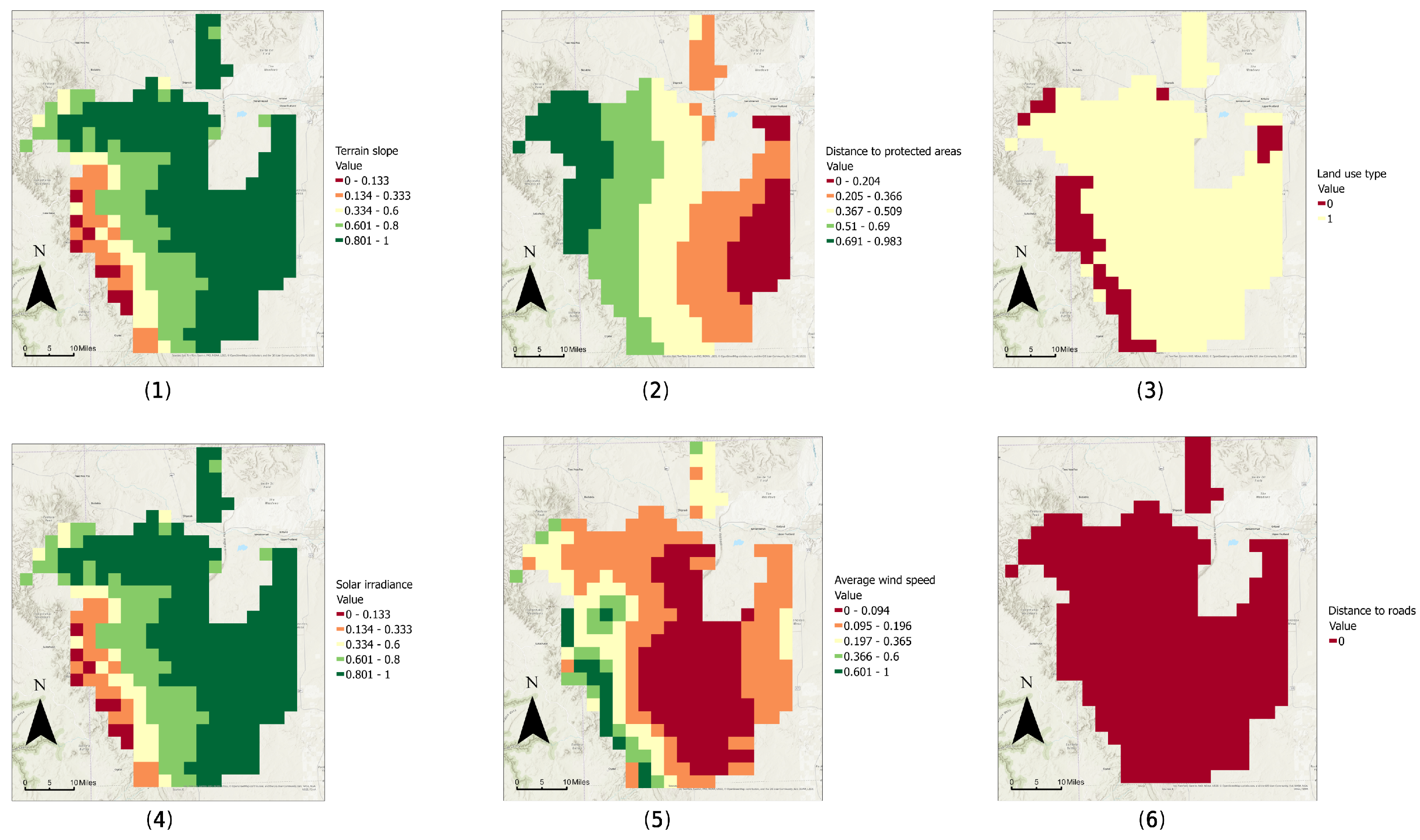
A set of spatial datasets was compiled to represent criteria including solar irradiance, average wind speed, land slope, land cover and buildability, distance to existing roads, and proximity to environmentally protected areas. Each layer was processed in ArcGIS Pro to ensure consistency, clipped to the study boundary of the Shiprock region and some surrounding chapters, projected to NAD 1983 UTM, and standardized to a common resolution. All layers were then normalized to a continuous scale between 0 and 1 in such a way that higher values consistently represented higher suitability. When necessary, the direction of preference was adjusted based on the type of variable. For instance, high solar and wind potential were assigned larger values, while lower values assigned to a steeper slope or areas located closer to protected regions. The land-use layer was handled slightly differently, where a binary indicator (suitable or not suitable) was created. Barren land, grassland, and shrub classifications were each considered suitable for microgrid placement and assigned a value of 1, whereas all other land-use types were classified as unsuitable, assigned a value of 0. Maps illustrating this processed spatial data are shown in Figure 2.
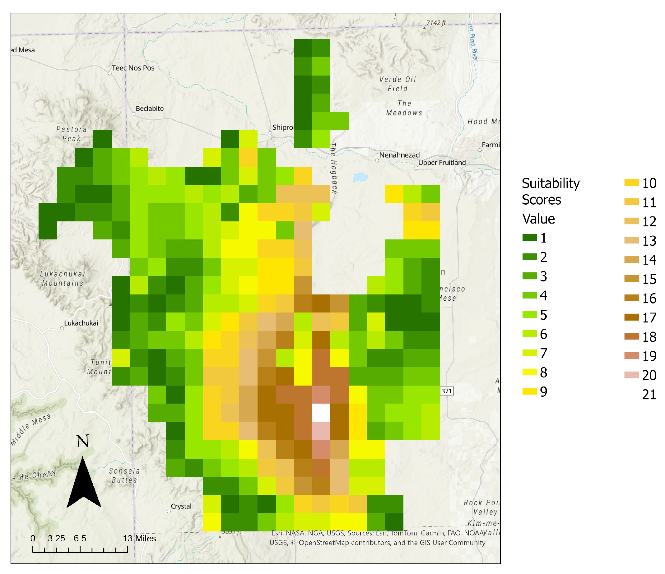
After applying the Pareto ranking algorithm, the resulting Pareto scores are obtained, which are visualized in Figure 3 to produce a Pareto-based suitability surface that highlights areas achieving the best overall balance among the evaluated criteria. Sites belonging to the different Pareto fronts represent locations for which improvements in one dimension (such as accessibility or resource potential) cannot be achieved without compromising another (such as slope or environmental sensitivity). This makes the Pareto ranking approach especially suitable for resilience and electrification studies, as it captures natural trade-offs among multiple spatial and sociotechnical factors.

4.3. Project Cost Analysis

In the optimization problem, the project cost is calculated using a net present cost (NPC) analysis. We assume that all annual repeated expenses are real costs, hence all project expenses can be discounted to the present using a real discount rate, which is assumed in this study to be r = 4 % . Of course, this value can vary depending on the project owner’s goals and surrounding financial environment. Without loss of generality, we assume that all construction happens during year zero, and the project’s useful lifetime S is 30 years. All technologies are assumed to have their own useful lifetimes during which they can be utilized, and at the end of which they need to be replaced. This is represented as the set of replacement years R , which includes year zero. The NPC of installing a certain capacity of each technology is a function of that technology’s installation cost, O&M costs, and fuel costs (if applicable), as described in Equation (18). The NPC of installing a new line is expressed in Equation (19).
NPC g = m M s R 1 ( 1 + r ) s C g cap · z m , g + s = 1 S 1 ( 1 + r ) s C m , g om · z m , g + t = 1 T 8760 T C m , g fuel · p m , g , t
NPC ( v ( i , d ) ) = s R 1 ( 1 + r ) s C cap · L ( j , d ) · v ( i , d ) + s = 1 S 1 ( 1 + r ) s C om · L ( i , d ) · v ( i , d )
Here, we assume that the analysis period T is representative of normal operating conditions, and thus fuel costs incurred during every hour in T can be projected to a full year’s fuel consumption using the scaling factor 8760 / T . The values for capital costs C g cap and C cap , operations and maintenance costs C m , g om and C om , and per-kWh fuel costs C m , g fuel , for generation technologies and lines respectively, are summarized in Table 2. The methodology and references used to obtain these values are described in Appendix B.

5. Results and Discussion

5.1. MCDM Results

The MCDM methodology is implemented using normalized geographical data corresponding to the study area. These datasets, as illustrated by Figure 2, are associated with criteria such as the availability of renewable resources and the suitability of the land within the region and illustrate the variability of these factors. Although some factors show higher suitability in certain regions, when all factors are combined within the MCDM framework, the final suitability of the land reflects the joint performance across all criteria under the Pareto-ranking scheme, without assigning subjective weights to any individual factor. For example, the slope of the terrain within this region is fairly suitable for microgrid development aside from the western region which consists of a local mountain range. Although this area corresponds to steeper terrain relative to the rest of the region, according to Figure 2(5), it corresponds to high wind availability. By incorporating both factors into our analysis, we can balance the tradeoffs between each of these factors in selecting proper sites for microgrid development. Figure 3 illustrates the final suitability as calculated using all criteria. In general, this map shows that the most suitable areas lie on the East and West sides of the region. This is not unexpected, as these areas are associated with high wind and solar availability. However, they are not without drawbacks. The West side of the region, as shown in Figure 2(3), is associated with land-uses unsuitable for development. It also has steep terrain, as shown in Figure 2(1). The East side of the region is located closer to protected areas, as depicted in Figure 2(2). In this analysis, we weigh each factor equally in order to avoid subjectivity. If, on the other hand, certain factors are deemed more important by the stakeholders, different weights can be assigned to different factors to reflect their corresponding importance in microgrid placement decisions.

5.2. Optimization Results

Problems P 1 , P 2 , P 3 , and P are solved for an analysis period of four days at an hourly resolution using the HiGHS solver with default settings. This four day period was chosen in order to consider representative variable generation production factors for four seasons, as described in Appendix B. For this problem instance, the program representing P has 63,766 rows, 42,746 columns, and 210 binary variables. The objective function values of interest, Q 1 , Q 2 , and Q 3 for each solution are summarized in Table 3, along with solution times for each run. From P 1 , the minimum cost solution to power at least ten percent of all unelectrified loads is 7.70 million USD. From P 2 , the minimum-emissions solution to power these loads is obtained as 1.0 kg CO2e. Finally, P 3 indicates that the maximum social-vulnerability-weighted load that can be met is 1879.20, which corresponds to 696 homes drawing 3 kVA at a power factor of 0.9. The result obtained for P represents a balance between the best-case scenarios for each objective. The final values for each objective function Q 1 , Q 2 , and Q 3 are 14.22 million USD, 1.85 kg CO2e, and 106 homes electrified, respectively. These values correspond to a change from each global optimal objective function, Δ ( Q n * ) , of 84.77% for all three objective functions.
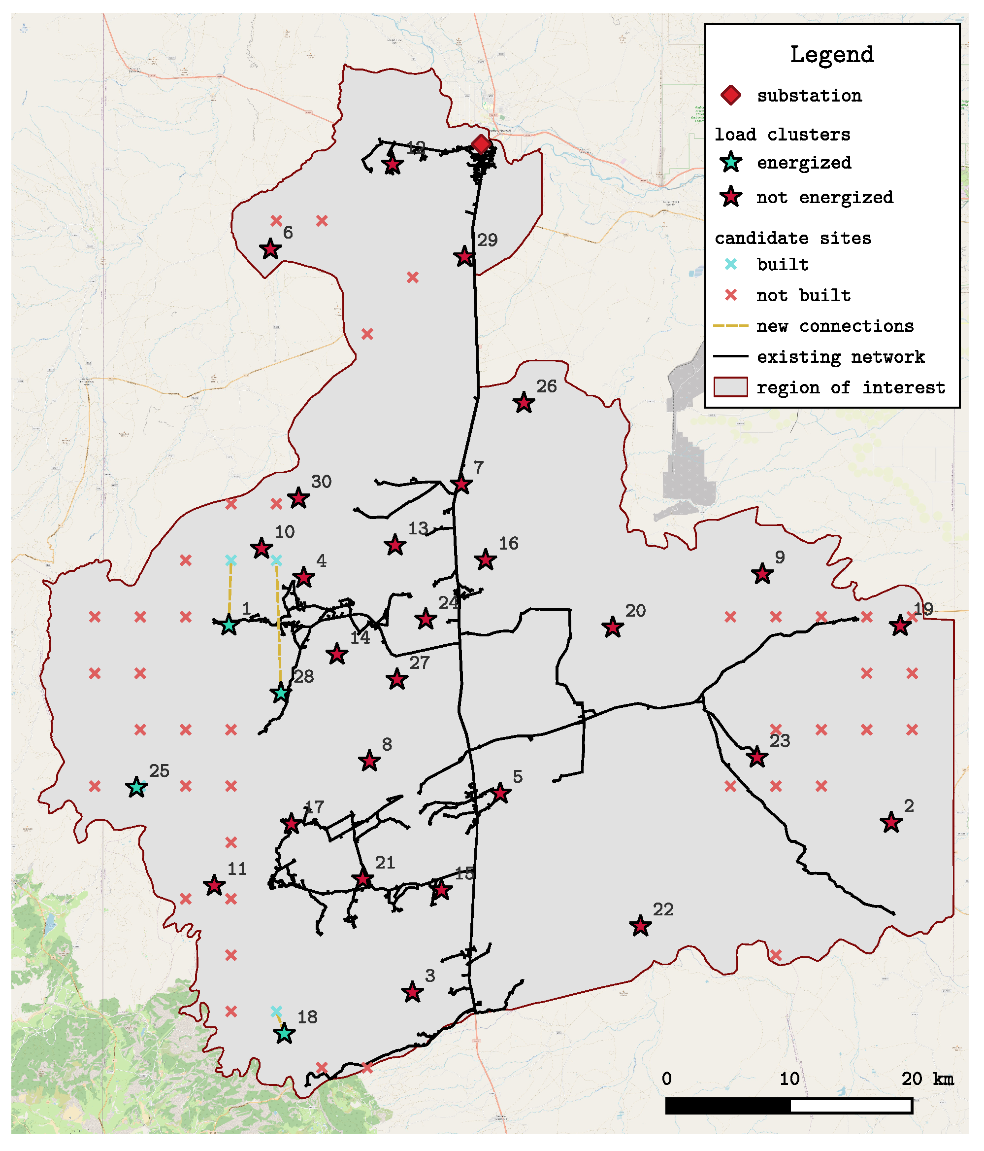
Table 4 gives a more detailed summary of the amount of each type of generation installed for each solution, as well as the number of microgrid connections and distribution extensions built. Of note, P 2 and P 3 both have very large values for most installations, as they are not cost-constrained problems. By contrast, the final solution to P installs primarily solar PV, wind, and storage capacity, along with a small amount of natural gas generation, across four microgrid sites, reflecting a cost- and emissions-efficient portfolio that still enables the electrification of a meaningful share of unelectrified households. A map showing the locations of constructed microgrids and lines connecting to energized demand nodes is provided in Figure 4.
Of note, solving P 1 leads to installing microgrids to energize load clusters 18 and 25. Because the largest component of project cost is driven by line installations, P 1 prioritizes energizing those loads first which have the shortest distance to either a microgrid candidate site or the distribution network. Beyond load clusters 18 and 25, the solution to the overall problem P suggests microgrids to energize load clusters 1 and 28. This is because energizing these loads provides an even tradeoff between the three objective functions of interest. There are larger load clusters which could be energized rather than these two, but the requisite cost or induced emissions associated with serving those alternatives outweighs the benefit of additional incremental electrification.
These results come with some limitations. First, for the Shiprock region, the social-vulnerability scores for every load cluster, which were obtained from [58], all have the same value as they were calculated using U.S. census data which does not offer sufficient granularity across the reservation. While this does not affect the generality of the proposed model, access to higher-granularity representations of social vulnerability or the cost of electricity not served across the region of study would lead to more practical results.
Further, our analysis indicates that the results are sensitive to user-defined parameter inputs. We consider most parameters, including cost parameters, emissions factors, and production factors as predetermined, without any arbitrary nature. However, the assumed baseline percentage of unserved load which must be met and the project discount rate must be selected (and are therefore not without selection bias), and their selection has an impact on the output of the model.
To demonstrate the model’s sensitivity to the selection of a baseline percentage of unserved load which must be met, we repeat the above analysis, changing only the assumption that at least ten percent of unserved households must be energized. Table 5 and Table 6 summarize the results when the above methodology is repeated, but with the minimum amount of newly served load set to 0.20.
From these tables, we observe that when the minimum threshold of electrified households is increased to 20%, Q 1 * (the value of Q 1 in the solution to P 1 ) more than doubles, while Q 2 * and Q 3 * remain unchanged from the solutions to the original problem. Therefore, the relative starting points for each optimal objective function value, used in Δ ( Q n * ) are different. As a result, the solution to the overall problem P results in Δ ( Q n * ) having a value of 71.69% for all three objective terms, which is significantly smaller than it was in the previous problem instance.
The discount rate r was also changed to demonstrate its impact on the overall solution. In effect, varying the discount rate only changes P 1 and P . A higher discount rate will make future expenses affect the present value of the project less, hence, we expect the optimal objective function value for P 1 to decrease as the discount rate is increased. To show that this is indeed the case, we reran the original problem instance for r values spanning from 0% to 10%, as the discount rate for most infrastructure projects should fall within this range. We summarize key results of this in Table 7. Here, it can be seen in the first column that Q 1 * does indeed decrease as r is increased. However, the final values for Δ ( Q 1 , 2 , 3 * ) , shown in the last column, do not increase substantially with an increase in the discount rate. From r = 0 to r = 10 , Δ ( Q 1 , 2 , 3 * ) increases by only 1.4368. Hence, this model is less sensitive to reasonable changes to the discount rate than it is to changes to the minimum electrification threshold. What the authors would like to emphasize from both of these sensitivity analyses is that it is important for planning entities which use this or any similar model to keep in mind the models’ sensitivity to user-defined inputs, and consider doing parameter sweeps before finalizing any decisions.
Another limitation of note is that because Q 3 * is large (1879.20 in this instance), a small change to Δ ( Q 3 * ) , which is reported as a percentage, can lead to a substantial change in the absolute value of Q 3 found in the final problem. This phenomenon is reflected in column 4 of Table 7, where variation in selection of the project’s discount rate from 2 to 10 percent can mean the difference between electrifying 109 and 99 homes (equivalent here to a final Q 3 value of 294.3 and 267.3, respectively). This is a direct consequence of prioritizing equal percentage deviations from optimal objective function values. In our case, this behavior is desirable because we seek to fairly balance the tradeoff between three objective functions of very different units and scales without the use of weights. However, this behavior should also be kept in mind when selecting a project discount rate to use as an input, because a small change to the discount rate can have an impact on the connectivity of tens of people.
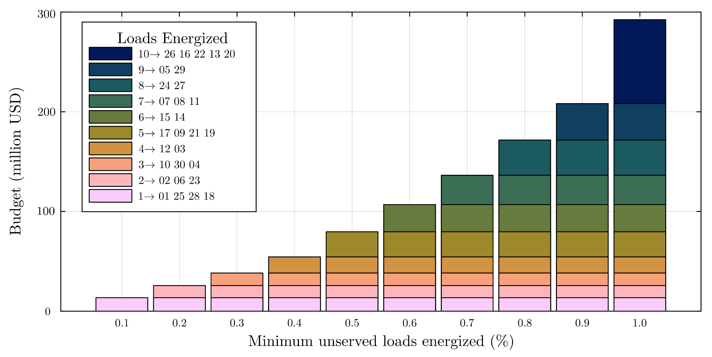
Interestingly, doing a parameter sweep of the minimum electrification threshold can give a sense of the action space for decision-makers using this model, given an uncertain constrained budget. We performed this parameter sweep, and show the results in Figure 5. Here, one can see that the additional marginal budget allocation required to energize each additional 10% increment of loads consistently increases. Energizing the final ten percent of loads costs more than five times the budget allocation required to energize the first ten percent of loads. It is important to emphasize that for this instance, because the social vulnerability scores for all loads in the region have the same value, this triage order strictly indicates an efficient path to rapid energization of loads given a limited budget. Repeated analysis with more granular social vulnerability scores should indicate the strategy to maximize social-vulnerability weighted load energization within limited budgets.

6. Conclusions

A multi-objective optimization framework was proposed in this paper for electrification of remote areas, considering both distribution grid extension and microgrid deployment as possible options. To narrow down microgrid candidate sites and create a tractable problem, a Pareto-ranking based multi-criteria decision making approach was developed and applied to allow for consideration of various suitability criteria such as resource availability, terrain, and proximity to roads, among others. Then, Chebyshev goal programming was adopted to balance three conflicting objectives, i.e., maximization of social-vulnerability-weighted energization of unelectrified loads, minimization of costs, and minimization of emissions. The applicability of the model was verified using a case study of the Shiprock region in the Navajo Nation, which offers an example of a large geographical region with suitably dispersed rural loads. The results indicate that the model manages to balance tradeoffs between the three objectives and prioritize energizing loads that can be met with the least-cost. The model and analysis proposed in this work can therefore inform local utilities in their planning as they consider the cost–benefit tradeoffs of increasing their budgets (on a one-time or annual basis) for remote electrification projects.
There is ample opportunity to extend this model as stakeholder needs dictate. For example, as it stands, this is a purely spatial model which does not incorporate detailed physical aspects such as line and transformer thermal limits, voltage drop constraints, or power losses. In order to consider these, the appropriate constraints may be added where needed. Future work addressing the appropriateness and granularity of generalized social vulnerability indices would also improve the usefulness of the proposed model. This model could provide more accurate results given more granular social vulnerability data, supposing that the metric used to produce said data adequately reflects the vulnerability of the populations being measured. This is a highly challenging problem which should be taken seriously by entities involved with utility network planning. Accuracy, granularity, and appropriateness of the social vulnerability data adopted are crucial because running a model and building a project based on a metric without all three of these characteristics runs the risk of excluding some of the very vulnerable stakeholders the project is meant to benefit.

Author Contributions

Conceptualization, S.M.; methodology, M.E.M., A.D., M.M.S., H.S., A.S. and S.M.; software, M.E.M., A.D., M.M.S. and H.S.; validation, M.E.M., A.D., M.M.S., H.S., A.S. and S.M.; formal analysis, M.E.M., A.D., M.M.S., H.S., A.S. and S.M.; investigation, M.E.M., A.D., M.M.S., H.S., A.S. and S.M.; data curation, M.E.M., A.D., M.M.S., H.S., A.S., M.I. and S.M.; writing—original draft preparation, M.E.M., A.D. and M.M.S.; writing—review and editing, A.S. and S.M.; visualization, M.E.M., A.D., M.M.S. and H.S.; supervision, M.I. and S.M. All authors have read and agreed to the published version of the manuscript.

Funding

Financial support from the Department of Energy (DOE) under the award number no. DE-EE0010420 for this research is gratefully acknowledged.

Institutional Review Board Statement

Not Applicable.

Informed Consent Statement

Not Applicable.

Data Availability Statement

Data used in this research has been obtained from publicly available sources and properly cited throughout the article.

Conflicts of Interest

The authors declare no conflict of interest.

Appendix A. Nomenclature

Table A1. Nomenclature for the optimization model.
Sets and Indices
b B Buses in the distribution network which are candidates for extension to unserved load areas
( b , d ) L 1 Set of directed arcs from buses in the distribution network to unserved load areas, representing candidate lines that can be built
d D Unserved load areas
g G Index for different types of generation technologies used in microgrids. In this study, the values of g = [1, 2, 3, 4, 5] correspond to generation types [diesel generators, gas generators, solar photovoltaic, wind turbines, 4-h chemical batteries]
i , j N Indices used to indicate nodes in the system. N = D M B
m M Microgrid candidate sites
( m , d ) L 2 Set of directed arcs from microgrid candidate sites to unserved load areas, representing candidate lines that can be built
t T Set of time steps considered in the problem
Parameters
C cap Capital costs associated with building a line, per unit of length
C g cap Capital costs associated with generation technology g
C m , g fuel Fuel costs associated with generation technology g in microgrid m
C om Operation and maintenance costs for a line, per unit of length
C m , g om Operation and maintenance costs for generation technology g in microgrid m
E g r i d Emissions due to the power delivered by the grid
E g Emission impact of generation type g
L ( i , d ) Length of line ( i , d )
MA sufficiently large number
P d Desired active power capacity at load area d
P m , g , t max Maximum allowable capacity of generator type g at microgrid site m at time t
rDiscount rate for net present value calculations
V d Social vulnerability score of load area d
Decision Variables
e m , t Energy contained by storage resource at microgrid site m at the end of time t
p d , t Total power provided to load d at time t
p d , t grid Power provided to load d by the distribution grid at time t
p d , t micro Power provided to load d by microgrids at time t
p ( i , d ) , t Power flow from node i to node d at time t
p m , g , t Power generation at microgrid site m using technology g at time t
u d Binary variable describing the decision to energize an unserved load area d. Value is 1 if the load is energized and 0 otherwise
v ( i , d ) Binary decision variable to construct a new line from node i to unserved load area d. Value is 1 if a line is constructed and 0 otherwise
z m , g Percentage of maximum capacity P m , g , t max of generation type g to build at microgrid site m. This is a number between 0 and 1

Appendix B. Cost and Emissions Accounting

Appendix B.1. Emissions Accounting

Emissions in this study are modeled as the amount of carbon dioxide equivalent emissions (kg CO2e), which are associated with the combustion of fuels (if applicable), as well as pre-combustion emissions representing possible fuel extraction and transport.

Appendix B.2. Distribution Network Extension

For electricity supplied from the grid, CO2e emissions are gathered from NREL’s Cambium 2024 database [66,67] using the default 2025 emissions rates (including pre-combustion, combustion, and T&D losses) for the WestConnectSouth region in the mid-case scenario. The average value is 333.8 kg CO2e/MWh. This value is used as the emissions factor E g r i d in the optimization model. We assume power costs for the utility to be 0.0276 USD/KWh, as reported in SPP’s State of the Market Report [68]. Although this utility is not a member of SPP, there is a DC tie line from an SPP region to the nearby grid. Accordingly, this price is used as a reasonable proxy for the marginal cost of imported electricity in the study area and is represented as the per-kWh fuel cost for imported power in the NPC calculations. For installation of new distribution lines, we assume a cost of 807,800 USD/km (as suggested in [69]).
Annual O&M costs were estimated based on 2019 FERC Form 1 [70,71] reported values for a small utility with approximately 109 circuit-miles of overhead lines. We use an estimated value of 60,000 USD/circuit-mile (37,120 USD/circuit-km).

Appendix B.3. Dispatchable Generation

Production factors for dispatchable generation are considered to be 1.0 for the entire analysis period. Based on the methodology presented in [72], we assume a CO2e value of 22.58 lb/gallon and 117.03 lb/MMBtu for diesel fuel and natural gas, respectively. A constant fuel price is assumed for natural gas at 4 USD/MMBtu [73] and for diesel at 4 USD/gallon [74]. For installation of generators, we based our analysis on current sales quotes for 30 kW and 150 kW diesel fuel and natural gas fuel generators [75,76,77,78]. We assume annual maintenance costs for generators based on numbers reported in [79]. We assume for a microgrid-capable diesel generator (150 kW rating for each unit), the generator will be running at around half capacity on average. Therefore, the specific fuel consumption is taken as 5.9 gallons/hour of diesel, or 1.152 MMBtu/hour of natural gas (from fuel consumption charts in [80]).

Appendix B.4. Variable Generation

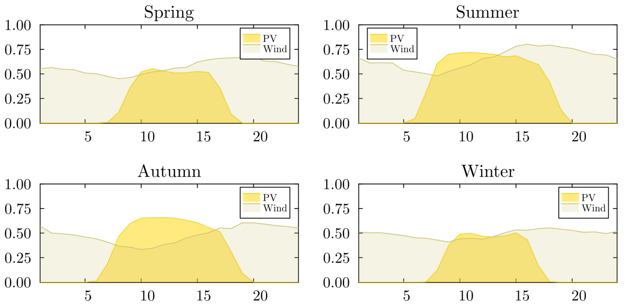
Production factors for solar PV generation were found using NREL’s PVWatts Calculator [81]. This resource provides an estimate of hourly production based on a given location and PV array type. Production factors for wind generation were derived using the WIND Toolkit within the Wind Resource Database [82]. Capital and O&M costs for PV, wind, and chemical storage are obtained from the 2024 NREL Annual Technology Baseline [83]. Similarly to [84,85], we aggregate these hourly production factors to create a representative 24-h period for each of four seasons in the year. This keeps the optimization problem tractable while allowing the incorporation of information provided by hourly weather data. Figure A1 shows the representative production factor profiles used in this study for the Navajo Reservation.
Figure A1. Seasonal representative 24-h production factors for Photovoltaic and Wind generation resources found for the Shiprock region. The x-axis represents time in hours and the y-axis represents the production factor.
Applsci 16 01227 g0a1
From [83], commercial-class (small microgrid-sized) ground-based PV is assumed to have a capital cost of 2567 USD/kW, and an O&M cost of 30 USD/kW-year. We assume a maximum allowable installation of 200 kW at any microgrid site, which corresponds to a land area of about 2 acres. Commercial-class wind is assumed to have a capital cost of 5398 USD/kW and an O&M cost of 38 USD/kW-year. We assume one turbine may be installed per microgrid site, which corresponds to a maximum of 250 kW installation.

Appendix B.5. Energy Storage

While in principle, energy storage and duration could be optimized separately, in this analysis we assume that all installed energy storage unit have a rated energy capacity of 4 h. This way, we can frame all costs in a per kWh basis. From [83], commercial Li-ion batteries are assumed to have a capital cost of 463.25 USD/kWh, and an O&M cost of 12.25 USD/kWh/year. We do not place a limit on the capacity of energy storage placed at a microgrid site.

References

  1. World Health Organization. Progress on Basic Energy Access Reverses for First Time in a Decade. 2024. Available online: https://www.who.int/news/item/12-06-2024-progress-on-basic-energy-access-reverses-for-first-time-in-a-decade (accessed on 23 April 2025).
  2. Beath, H.; Alonso, J.B.; Mori, R.; Gambhir, A.; Nelson, J.; Sandwell, P. Maximising the benefits of renewable energy infrastructure in displacement settings: Optimising the operation of a solar-hybrid mini-grid for institutional and business users in Mahama Refugee Camp, Rwanda. Renew. Sustain. Energy Rev. 2023, 176, 113142. [Google Scholar] [CrossRef] [Scilit]
  3. Bekele, A.; Khan, B.; Zdiri, M.A.; Guerrero, J.M.; Chaudhary, S.; Vasquez, J.C.; Agundis Tinajero, G.D. Optimal Planning and Sizing of Microgrid Cluster for Performance Enhancement. Sci. Rep. 2024, 14, 26653. [Google Scholar] [CrossRef] [Scilit]
  4. Tafula, J.E.; Justo, C.D.; Moura, P.; Mendes, J.; Soares, A. Multicriteria Decision-Making Approach for Optimum Site Selection for Off-Grid Solar Photovoltaic Microgrids in Mozambique. Energies 2023, 16, 2894. [Google Scholar] [CrossRef] [Scilit]
  5. Zhao, H.; Guo, S.; Zhao, H. Selecting the Optimal Micro-Grid Planning Program Using a Novel Multi-Criteria Decision Making Model Based on Grey Cumulative Prospect Theory. Energies 2018, 11, 1840. [Google Scholar] [CrossRef] [Scilit]
  6. Daeli, A.; Mohagheghi, S. Power Grid Infrastructural Resilience against Extreme Events. Energies 2023, 16, 64. [Google Scholar] [CrossRef] [Scilit]
  7. Tribal Electricity Access and Reliability: Report to Congress. August 2023. Available online: https://www.energy.gov/sites/default/files/2024-01/EXEC-2023-000952%20-%20Tribal%20Electricity%20Access%20Reliability%20Report%20to%20Congress%20%28Final%20Draft%20-%20Clean%29-signed%20by%20S1.pdf (accessed on 1 January 2026).
  8. Enhancing Power Grid Resilience for Navajo Nation, Department of Civil, Environmental and Geodetic Engineering, The Ohio State University. Available online: https://ceg.osu.edu/news/2023/09/enhancing-power-grid-resilience-navajo-nation (accessed on 1 January 2026).
  9. Billanes, J.D.; Jørgensen, B.N.; Ma, Z. A Framework for Resilient Community Microgrids: Review of Operational Strategies and Performance Metrics. Energies 2025, 18, 405. [Google Scholar] [CrossRef] [Scilit]
  10. Wang, C.; Cheng, B.; He, X.; Xi, L.; Yang, N.; Zhao, Z.; Lai, C.S.; Lai, L.L. Integrated Underfrequency Load Shedding Strategy for Islanded Microgrids Integrating Multiclass Load-Related Factors. IEEE Trans. Smart Grid 2025, 16, 4305–4323. [Google Scholar] [CrossRef] [Scilit]
  11. Energizing Navajo Nation: How Electrification Can Secure a Sustainable Future for Indian Country. July 2021. Available online: https://www.brookings.edu/articles/energizing-navajo-nation-how-electrification-can-secure-a-sustainable-future-for-indian-country/ (accessed on 1 January 2026).
  12. Begay, S.K. Navajo residential solar energy access as a global model. Electr. J. 2018, 31, 9–15. [Google Scholar] [CrossRef] [Scilit]
  13. The Navajo Nation Tribal Government-Kayenta Chapter—2022 Project, Department of Energy. December 2022. Available online: https://www.energy.gov/sites/default/files/2022-12/1-navajo-nation-keyenta.pdf (accessed on 1 January 2026).
  14. Khlifi, F.; Cherif, H.; Belhadj, J. Environmental and economic optimization and sizing of a micro-grid with battery storage for an industrial application. Energies 2021, 14, 5913. [Google Scholar] [CrossRef] [Scilit]
  15. Suresh, V.; Muralidhar, M.; Kiranmayi, R. Modelling and optimization of an off-grid hybrid renewable energy system for electrification in a rural areas. Energy Rep. 2020, 6, 594–604. [Google Scholar] [CrossRef] [Scilit]
  16. Rodriguez, R.; Osma, G.; Ordoñez, G. Sizing of a Scattered Housing Microgrid in a Remote Rural Area. Renew. Energy Power Qual. J. 2022, 20, 43–48. [Google Scholar] [CrossRef] [Scilit]
  17. Wang, Y.; Wang, X.; Yu, H.; Huang, Y.; Dong, H.; Qi, C.; Baptiste, N. Optimal design of integrated energy system considering economics, autonomy and carbon emissions. J. Clean. Prod. 2019, 225, 563–578. [Google Scholar] [CrossRef] [Scilit]
  18. Hosseini, S.J.A.D.; Moazzami, M.; Shahinzadeh, H. Optimal Sizing of an Isolated Hybrid Wind/PV/Battery System with Considering Loss of Power Supply Probability. Majlesi J. Electr. Eng. 2017, 11, 63–69. [Google Scholar]
  19. Budiman, F.N.; Ramli, M.A.M.; Bouchekara, H.R.E.H.; Milyani, A.H. Optimal scheduling of a microgrid with power quality constraints based on demand side management under grid-connected and islanding operations. Int. J. Electr. Power Energy Syst. 2024, 155, 109650. [Google Scholar] [CrossRef] [Scilit]
  20. Ahmadipour, M.; Othman, M.M.; Salam, Z.; Alrifaey, M.; Ridha, H.M.; Veerasamy, V. Optimal load shedding scheme using grasshopper optimization algorithm for islanded power system with distributed energy resources. Ain Shams Eng. J. 2023, 14, 101835. [Google Scholar] [CrossRef] [Scilit]
  21. Hussain, A.; Kim, H.M. Goal-programming-based multi-objective optimization in off-grid microgrids. Sustainability 2020, 12, 8119. [Google Scholar] [CrossRef] [Scilit]
  22. Dougier, N.; Garambois, P.; Gomand, J.; Roucoules, L. Multi-objective non-weighted optimization to explore new efficient design of electrical microgrids. Appl. Energy 2021, 304, 117758. [Google Scholar] [CrossRef] [Scilit]
  23. Lan, H.; Wen, S.; Hong, Y.Y.; Yu, D.C.; Zhang, L. Optimal sizing of hybrid PV/diesel/battery in ship power system. Appl. Energy 2015, 158, 26–34. [Google Scholar] [CrossRef] [Scilit]
  24. Dufo-López, R.; Cristóbal-Monreal, I.R.; Yusta, J.M. Optimisation of PV-wind-diesel-battery stand-alone systems to minimise cost and maximise human development index and job creation. Renew. Energy 2016, 94, 280–293. [Google Scholar] [CrossRef] [Scilit]
  25. Silva, D.; Nakata, T. Multi-objective assessment of rural electrification in remote areas with poverty considerations. Energy Policy 2009, 37, 3096–3108. [Google Scholar] [CrossRef] [Scilit]
  26. Petrelli, M.; Fioriti, D.; Berizzi, A.; Poli, D. Multi-Year Planning of a Rural Microgrid Considering Storage Degradation. IEEE Trans. Power Syst. 2021, 36, 1459–1469. [Google Scholar] [CrossRef] [Scilit]
  27. Petrelli, M.; Fioriti, D.; Berizzi, A.; Bovo, C.; Poli, D. A novel multi-objective method with online Pareto pruning for multi-year optimization of rural microgrids. Appl. Energy 2021, 299, 117283. [Google Scholar] [CrossRef] [Scilit]
  28. Malheiro, A.; Castro, P.M.; Lima, R.M.; Estanqueiro, A. Integrated sizing and scheduling of wind/PV/diesel/battery isolated systems. Renew. Energy 2015, 83, 646–657. [Google Scholar] [CrossRef] [Scilit]
  29. Zhang, Q.; Ding, J.; Shen, W.; Ma, J.; Li, G. Multiobjective Particle Swarm Optimization for Microgrids Pareto Optimization Dispatch. Math. Probl. Eng. 2020, 2020, 5695917. [Google Scholar] [CrossRef] [Scilit]
  30. Kassab, F.A.; Celik, B.; Locment, F.; Sechilariu, M.; Hansen, T.M. Combined Optimal Sizing and Energy Management of a DC Microgrid using MILP. In Proceedings of the 2023 IEEE Belgrade PowerTech (PowerTech 2023), Belgrade, Serbia, 25–29 June 2023; IEEE: Piscataway, NJ, USA, 2023. [Google Scholar] [CrossRef] [Scilit]
  31. Kassab, F.A.; Celik, B.; Locment, F.; Sechilariu, M. Optimal Sizing of an Isolated DC Microgrid Using Multiobjective Optimization with Linear Programming. Available online: https://hal.science/hal-03775487v1 (accessed on 23 April 2025).
  32. Rezvani, A.; Gandomkar, M.; Izadbakhsh, M.; Ahmadi, A. Environmental/economic scheduling of a micro-grid with renewable energy resources. J. Clean. Prod. 2015, 87, 216–226. [Google Scholar] [CrossRef] [Scilit]
  33. Nikmehr, N.; Ravadanegh, S.N. Optimal Power Dispatch of Multi-Microgrids at Future Smart Distribution Grids. IEEE Trans. Smart Grid 2015, 6, 1648–1657. [Google Scholar] [CrossRef] [Scilit]
  34. Dehghani, N.L.; Shafieezadeh, A. Multi-stage resilience management of smart power distribution systems: A stochastic robust optimization model. IEEE Trans. Smart Grid 2022, 13, 3452–3467. [Google Scholar] [CrossRef] [Scilit]
  35. Ding, B.; Li, Z.; Li, Z.; Xue, Y.; Chang, X.; Su, J.; Jin, X.; Sun, H. A CCP-based distributed cooperative operation strategy for multi-agent energy systems integrated with wind, solar, and buildings. Appl. Energy 2024, 365. [Google Scholar] [CrossRef] [Scilit]
  36. Emerging Grid Objectives and Multi-Objective Decision Planning (MOD-Plan), Sandia National Laboratories. October 2021. Available online: https://www.sandia.gov/app/uploads/sites/273/2021/10/Emerging-Grid-Objectives-and-Multi-Objective-Planning_Project-Overview_July-2021_3.pdf (accessed on 1 January 2026).
  37. Zhu, X.; Ruan, G.; Geng, H.; Liu, H.; Bai, M.; Peng, C. Multi-Objective Sizing Optimization Method of Microgrid Considering Cost and Carbon Emissions. IEEE Trans. Ind. Appl. 2024, 60, 5565–5576. [Google Scholar] [CrossRef] [Scilit]
  38. Cheraghi, R.; Hossein Jahangir, M. Multi-objective optimization of a hybrid renewable energy system supplying a residential building using NSGA-II and MOPSO algorithms. Energy Convers. Manag. 2023, 294, 117515. [Google Scholar] [CrossRef] [Scilit]
  39. Alzahrani, A.; Hayat, M.A.; Khan, A.; Hafeez, G.; Khan, F.A.; Khan, M.I.; Ali, S. Optimum sizing of stand-alone microgrids: Wind turbine, solar photovoltaic, and energy storage system. J. Energy Storage 2023, 73, 108611. [Google Scholar] [CrossRef] [Scilit]
  40. Katsigiannis, Y.A.; Georgilakis, P.S.; Karapidakis, E.S. Hybrid simulated annealing-tabu search method for optimal sizing of autonomous power systems with renewables. IEEE Trans. Sustain. Energy 2012, 3, 330–338. [Google Scholar] [CrossRef] [Scilit]
  41. Farnaz; Nuthammachot, N.; Shabbir, R. Evaluating site selection for optimal photovoltaic installations and CO2 emission reduction in selected districts of Khyber Pakhtunkhwa. Sci. Rep. 2025, 15, 6635. [Google Scholar] [CrossRef] [Scilit]
  42. Zhang, X.A.; Kinder, P.; Strager, M.; Taylor, S.; Schwartzman, G. Distributed energy infrastructure development: Geospatial and economic feasibility in rural West Virginia. In Environment, Development and Sustainability; Springer: Berlin/Heidelberg, Germany, 2024; pp. 1–38. [Google Scholar] [CrossRef] [Scilit]
  43. Solangi, Y.A.; Shah, S.A.A.; Zameer, H.; Ikram, M.; Saracoglu, B.O. Assessing the solar PV power project site selection in Pakistan: Based on AHP-fuzzy VIKOR approach. Environ. Sci. Pollut. Res. 2019, 26, 30286–30302. [Google Scholar] [CrossRef] [Scilit] [PubMed]
  44. Bohra, S.S.; Anvari-Moghaddam, A.; Blaabjerg, F.; Mohammadi-Ivatloo, B. Multi-criteria planning of microgrids for rural electrification. J. Smart Environ. Green Comput. 2021, 1, 120–134. [Google Scholar] [CrossRef] [Scilit]
  45. Gómez-Hernández, D.F.; Domenech, B.; Juanpera, M.; Ferrer-Martí, L. Ranking projects in regional electrification plans considering technical and social criteria. Case study in Mexico. Energy Sustain. Dev. 2023, 77, 101336. [Google Scholar] [CrossRef] [Scilit]
  46. Mosetlhe, T.; Babatunde, O.; Yusuff, A.; Ayodele, T.; Ogunjuyigbe, A. A MCDM approach for selection of microgrid configuration for rural water pumping system. Energy Rep. 2023, 9, 922–929. [Google Scholar] [CrossRef] [Scilit]
  47. Prum, M.; Goh, H.H.; Zhang, D.; Dai, W.; Kurniawan, T.A.; Goh, K.C. Optimizing hybrid energy systems for remote communities in Asia’s least developed countries. Heliyon 2024, 10, e29369. [Google Scholar] [CrossRef] [Scilit]
  48. Yathip, B.; Usapein, P.; Madtharad, C.; Jirawongnusorn, S. A multi-criteria decision analysis to rank energy alternative options using analytic hierarchy process with a sustainable criteria: A case study of Mae Sariang, Mae Hon Song Province, Thailand. J. Infrastruct. Policy Dev. 2024, 2024, 5565. [Google Scholar] [CrossRef] [Scilit]
  49. Azad, A.M.A.S.; Oishi, Z.T.; Islam, M.A.; Islam, M.R. Advancing Economical and Environmentally Conscious Electrification: A Comprehensive Framework for Microgrid Design in Off-Grid Regions. Glob. Challenges 2024, 8, 2400169. [Google Scholar] [CrossRef] [Scilit]
  50. Rygel, L.; O’sullivan, D.; Yarnal, B. A Method for Constructing a Social Vulnerability Index: An Application to Hurricane Storm Surges in a Developed Country. Mitig. Adapt. Strateg. Glob. Change 2006, 11, 741–764. [Google Scholar] [CrossRef] [Scilit]
  51. US EPA. U.S. PAD-US Protected Areas (USGS & ESRI 2020). 2022. Available online: https://www.arcgis.com/home/item.html?id=30a56c26b85741b5a4604315d193f9e1 (accessed on 1 January 2026).
  52. NREL. Solar Resource, NSRDB PSM Global Horizontal Irradiance (GHI)—North American Cooperation on Energy Information. 2018. Available online: https://www.nrel.gov/gis/solar-resource-maps (accessed on 1 January 2026).
  53. ESRI. USA NLCD Land Cover. 2023. Available online: https://landscape10.arcgis.com/arcgis/rest/services/USA_NLCD_Land_Cover/ImageServer (accessed on 1 January 2026).
  54. ESRI. Terrain—Slope Map. 2025. Available online: https://elevation.arcgis.com/arcgis/rest/services/WorldElevation/Terrain/ImageServer (accessed on 1 January 2026).
  55. NREL. USA Average Wind Speed (Elevation 10-m to 200-m). 2025. Available online: https://tiledimageservices.arcgis.com/P3ePLMYs2RVChkJx/arcgis/rest/services/US_Annual_Average_Wind_Speed/ImageServer (accessed on 1 January 2026).
  56. U.S. Census Bureau. TIGER/Line Shapefiles. 2024. Available online: https://www.census.gov/geographies/mapping-files/time-series/geo/tiger-line-file.html (accessed on 23 May 2024).
  57. Dugan, J.; Byles, D.; Mohagheghi, S. Social Vulnerability to Long-Duration Power Outages. Int. J. Disaster Risk Reduct. 2023, 85, 103501. [Google Scholar] [CrossRef] [Scilit]
  58. Dugan, J.; Mohagheghi, S. Assessment of Social Vulnerability to Long-Duration Power Outages in the United States. In Proceedings of the 2023 IEEE Green Technologies Conference (GreenTech), Denver, CO, USA, 19–21 April 2023. [Google Scholar] [CrossRef] [Scilit]
  59. Indian Health Service (IHS). Indian Health Service Facility Locations. 2023. Available online: https://ihs.gov/locations/ (accessed on 1 January 2026).
  60. New Mexico Public Education Department. New Mexico Public School Directory. Available online: https://web.ped.nm.gov/bureaus/constituent-services/school-directory/ (accessed on 1 January 2026).
  61. Navajo Nation Division of Community Development. Navajo Nation ASC Map. 2024. Hosted on ArcGIS. Available online: https://www.arcgis.com/home/item.html?id=db69242bd4db4d52bfae9b9d713b775e (accessed on 23 May 2024).
  62. Federal Emergency Management Agency (FEMA). USA Structures. 2024. Available online: https://gis-fema.hub.arcgis.com/pages/usa-structures (accessed on 23 May 2024).
  63. Chattopadhyay, A.; Witmer, A.P. Practical energy equity decision making in resource-constrained communities: A case study in the Navajo Nation. Electr. J. 2025, 38, 107456. [Google Scholar] [CrossRef] [Scilit]
  64. Bickel, J.A.; Naishadham, S. On Navajo Nation, a Push to Electrify More Homes on the Vast Reservation. 2024. Available online: https://ictnews.org/news/on-navajo-nation-a-push-to-electrify-more-homes-on-the-vast-reservation/ (accessed on 12 January 2026).
  65. Fang, Y.; Wang, J. Selection of the number of clusters via the bootstrap method. Comput. Stat. Data Anal. 2012, 56, 468–477. [Google Scholar] [CrossRef] [Scilit]
  66. NREL. Cambium 2024. Available online: https://scenarioviewer.nrel.gov (accessed on 15 October 2025).
  67. Cambium 2024 Scenario Descriptions and Documentation. 2024. Available online: https://docs.nrel.gov/docs/fy25osti/93005.pdf (accessed on 15 October 2025).
  68. SPP State of the Market 2024. 2024. Available online: https://www.spp.org/documents/73953/2024_annual_state_of_the_market_report.pdf (accessed on 15 October 2025).
  69. Distributed Energy Resources (DER) Project Costs. 2022. Available online: https://www.eversource.com/residential/about/doing-business-with-us/interconnections/massachusetts/distributed-energy-resources-project-costs (accessed on 1 January 2026).
  70. Fares, R.; King, C. FERC Form 1 Electric Utility Cost, Energy Sales, Peak Demand, and Customer Count Data 1994–2019. Open Energy Data Initiative (OEDI), National Renewable Energy Laboratory. 2017. Available online: https://data.openei.org/submissions/489 (accessed on 31 December 2025).
  71. Connecticut Siting Council Investigation into the Life-Cycle Costs of Electric Transmission Lines. 2017. Available online: https://portal.ct.gov/-/media/csc/publications/2017lifecyclefinalrptpdf.pdf?rev=ab8d4f516aa640848882497b5dbcdde4&hash=8FEAFCE8F3E5E67DCEFB2F395D2A9147 (accessed on 1 January 2026).
  72. Anderson, K.; Olis, D.; Becker, B.; Casson, L.; Laws, N.; Li, X.; Mishra, S.; Jeffery, A.; Elgqvist, E.; Krah, K.; et al. The REopt Web Tool User Manual. Available online: https://reopt.nrel.gov/tool/reopt-user-manual.pdf (accessed on 15 October 2025).
  73. EIA Henry Hub Natural Gas Price. 2025. Available online: https://www.eia.gov/dnav/ng/hist/rngwhhdA.htm (accessed on 15 October 2025).
  74. EIA Gasoline and Diesel Fuel Update. 2025. Available online: https://www.eia.gov/petroleum/gasdiesel/ (accessed on 15 October 2025).
  75. Electric Generators Direct. 30 kW Generators. Available online: https://www.electricgeneratorsdirect.com/power/30-kw-generators.html (accessed on 1 January 2026).
  76. Cummins 30 kW C30D6 Diesel Whole House Generator. 2025. Available online: https://buckeyepowersystems.com/products/cummins-30kw-diesel-c30d6-120-240v?srsltid=AfmBOop8E0EURCS0nN5fjTdAig3lAgYfZUl5ievGsQdxiGrg8CdEy6Id (accessed on 15 October 2025).
  77. Cummins Ag Spec 150 kW Open Diesel Generator (120/240 V Single-Phase). 2025. Available online: https://www.fergusonhome.com/cummins/c82047642 (accessed on 1 January 2026).
  78. Nationwide Generators. 2022. Available online: https://www.nationwidegenerators.com/70kw-to-150kw/?srsltid=AfmBOopYmp04nH6zVF7DehknSVNV0CLTGmCB8IF5RrHfVpWM9T17gWHJ (accessed on 15 October 2025).
  79. Natural Gas Generator Cost Guide for Business & Industry. 2025. Available online: https://www.depco.com/blog/cost-of-natural-gas-generators/#:~:text=Most%20manufacturers%20recommend%20scheduled%20service,response%20time%20and%20preventive%20care (accessed on 15 October 2025).
  80. Diesel & Natural Gas Generator Fuel Consumption Charts. 2025. Available online: https://generatorsource.com/tools-info/fuel-consumption-charts/ (accessed on 15 October 2025).
  81. PVWatts® Calculator Version 8.0. 2025. Available online: https://pvwatts.nrel.gov/pvwatts.php (accessed on 15 October 2025).
  82. Draxl, C.; Clifton, A.; Hodge, B.M.; McCaa, J. The Wind Integration National Dataset (WIND) Toolkit. Appl. Energy 2015, 151, 355–366. [Google Scholar] [CrossRef] [Scilit]
  83. NREL. Electricity Annual Technology Baseline. 2024. Available online: https://atb.nrel.gov/electricity/2024/data (accessed on 15 October 2025).
  84. Mai, T.; Brown, P.R.; Lavin, L.; Dhulipala, S.C.; Kuna, J. Incorporating Stressful Grid Conditions for Reliable and Cost-Effective Electricity System Planning. SSRN 2024. [Google Scholar] [CrossRef] [Scilit]
  85. Brown, P.R.; Cole, W.J.; Mai, T. An interregional optimization approach for time series aggregation in continent-scale electricity system models. Energy 2025, 324, 135830. [Google Scholar] [CrossRef] [Scilit]
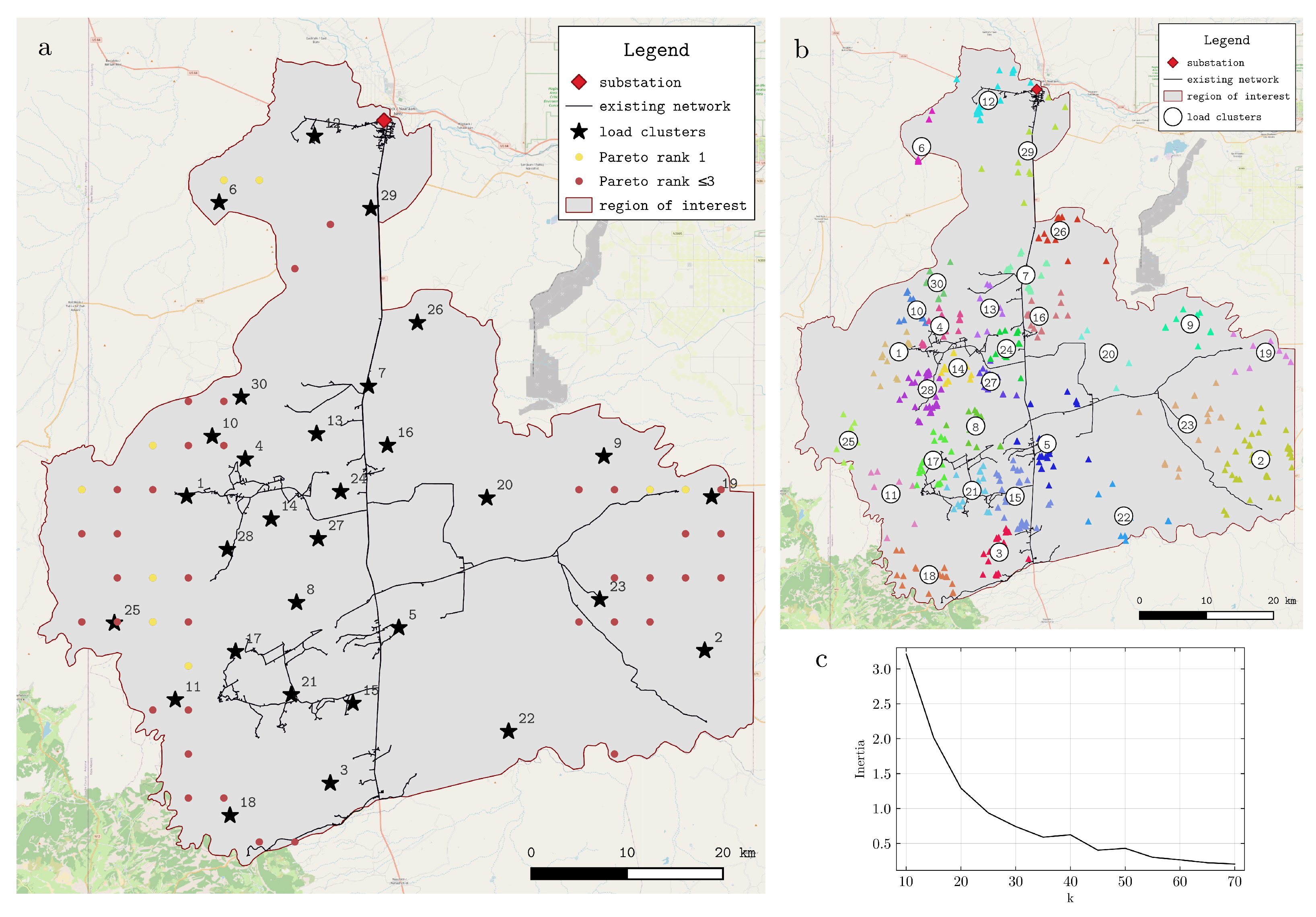
Figure 1. (a). Synthetic network representing the electric distribution grid of the Shiprock region in the Navajo Nation, with microgrid candidate sites and load cluster centroids. (b). K-means clustering of buildings, with k = 30. Triangles indicate individual loads and numbered circles indicate clusters. Different colors have been used associated with each cluster. (c). Inertia plot for k-means clustering of buildings.
Applsci 16 01227 g001
Figure 2. Normalized (1). slope values, (2). distance to protected areas, (3). land-use classifications, (4). average solar irradiance, (5). average wind speed, and (6). distance to roads across the study region.
Applsci 16 01227 g002
Figure 3. Visualization of Pareto ranking across the entire study area. A lower suitability score means a higher ranking i.e., a suitability score of 1 signifies a more suitable site for microgrid placement and a score of 21 means the area is the least suitable site for microgrid placement.
Applsci 16 01227 g003
Figure 4. Results to multi-objective optimization problem P .
Applsci 16 01227 g004
Figure 5. Priority order of load cluster energization. Under a generic budget, loads 1, 25, 28, and 18 should be energized first, after which loads 2, 6, and 23 should be energized, and so on.
Applsci 16 01227 g005
Table 1. Comparison of Multi-Criteria Considerations in Microgrid Planning Studies. Econ. = Economic, Env. = Environmental, Tech. = Technical, Soc. = Social.
StudyEcon.Env.Tech.Soc.Application/Context
[43]PV microgrid siting across 14 cities in Pakistan.
[44] Hybrid microgrid (PV, wind, hydro, biogas) in Arusha, Tanzania.
[45] Electrification prioritization in 8 off-grid communities in Chiapas, Mexico.
[4]Off-grid solar microgrid siting in Mozambique.
[46] Optimal microgrid setup for water pumping systems.
[47] Hybrid system optimization in four less developed countries in Asia including Cambodia and Laos.
[48]Microgrid expansion planning in Mae Sariang, Thailand.
[49] Sustainable microgrid design in off-grid South Asia.
Table 2. Summary of parameter inputs.
Capital CostO&M CostFuel CostEmissionsMax InstallationReplacement Year
USD/kW USD/kW/yr USD/kWh kgCO2e/kWh kW Years
Line Construction0.8078 10.25 1--->30
Imported Power--0.02760.3338 -
Natural Gas302.46100.06140.8153-5–10
Diesel236.84100.31470.8057-5–10
Solar PV179518--20025–30
Wind539838--25020–25
Chemical battery 2463.25 312 3---10–15
1  10 6 USD/km, 10 6 USD/km/yr; 2 Assuming a 4-h duration Li-ion battery; 3 USD/kWh, USD/kWh/yr.
Table 3. Solution objective function values and compute times. Highlighted cells correspond to terms included in each problem’s overall objective function.
Model Q 1 Q 2 Q 3 Compute Time
10 6 USD kg CO2e SV kWh Met s
P 1 7.7014,792.80189.002.1332
P 2 3469.461.001879.200.1466
P 3 3457.05145,350.861879.200.1407
P 14.221.85286.2089.987
Table 4. Result installation summaries. NG—natural gas, DI—diesel, PV—solar photovoltaic, WI—wind, BT—battery storage.
Total Installed GenerationConnections
NG (kW) DI (kW) PV (kW) WI (kW) BT (kW) Microgrid Distribution
P 1 189.000.000.000.000.0020
P 2 0.000.008800.0011,000.0019,538.5915030
P 3 0.002497.508800.0011,000.000.0015030
P 0.230.00208.30504.2897.7840
Table 5. Solution objective function values and compute times when the threshold for minimum electrification is set to 0.20. Highlighted cells correspond to terms included in each problem’s overall objective function.
Model Q 1 Q 2 Q 3 Compute Time
10 6 USD kg CO2e SV kWh Met s
P 1 15.8030,008.26383.402.8860
P 2 3469.461.001879.200.1332
P 3 3457.05145,350.861879.200.1439
P 27.131.72531.90139.0230
Table 6. Result installation summaries when the threshold for minimum electrification is set to 0.20. NG—natural gas, DI—diesel, PV—solar photovoltaic, WI—wind, BT—battery storage.
Total Installed GenerationConnections
NG (kW) DI (kW) PV (kW) WI (kW) BT (kW) Microgrid Distribution
P 1 383.400.000.000.000.0040
P 2 0.000.008800.0011,000.0019,538.5915030
P 3 0.002497.508800.0011,000.000.0015030
P 0.970.00510.94913.17226.7360
Table 7. Key objective function values from running the proposed optimization routine with varying values for the discount rate r. Objective function values for P 2 and P 3 are excluded because they do not change when r is varied.
r (%) P 1 , Q 1 * P , Q 1 P , Q 2 P , Q 3 Δ ( Q 1 , 2 , 3 * )
011.0220.311.84294.3084.3391%
29.0316.651.84294.3084.3391%
47.7014.221.85286.2084.7701%
66.7812.551.85278.1085.2011%
86.1211.341.85278.1085.2011%
105.6510.491.86267.3085.7759%
Disclaimer/Publisher’s Note: The statements, opinions and data contained in all publications are solely those of the individual author(s) and contributor(s) and not of MDPI and/or the editor(s). MDPI and/or the editor(s) disclaim responsibility for any injury to people or property resulting from any ideas, methods, instructions or products referred to in the content.